ASIANPAINT 1 Week Time Frame 📊 Current Price Context
Recent share price was trading around ₹2,423–₹2,515 range (latest intraday/previous close range) according to market data.
📈 Weekly Timeframe Levels — Asian Paints (NSE)
🔴 Resistance (Upside)
These are levels where price may face selling pressure or pause on the upside in the coming week:
1. ₹2,560–₹2,565 — Immediate near‑term resistance zone seen from short weekly consolidations.
2. ₹2,720–₹2,760 — Mid resistance zone where upside moves often stall on weekly/daily clusters.
3. ₹2,820–₹2,860+ — Higher weekly resistance zone — breakout above this could indicate stronger momentum.
🟢 Support (Downside)
These are levels where price might find buying interest or a floor on weekly charts:
1. ₹2,440–₹2,460 — Immediate support from weekly lower bands and short pivot support.
2. ₹2,340–₹2,380 — Secondary support zone seen from historical price clusters and volatility bands.
3. ₹2,300–₹2,250 — Major structural support — breakdown here could lead to deeper correction.
📉 Pivot Zone
₹2,500–₹2,530 — A central pivot/neutral range this week; trading above suggests short bullish bias, below suggests bearish.
📌 Weekly Technical Bias (Summary)
Bullish Scenario: A sustained weekly close above ₹2,560–₹2,565 opens path toward ₹2,720–₹2,860.
Bearish Scenario: Failure to hold ₹2,440–₹2,460 could drag price toward ₹2,340–₹2,300 on the weekly chart.
Range Play: Price oscillating between ₹2,440 – ₹2,560 indicates consolidative behavior typical in neutral markets.
Chart Patterns

FUSION - Time to shine?DISCLAIMER: This is NOT a trade recommendation but only my observation. Please do your own analysis before entering your trades
Points to note:
-----------------
1. Price has been in consolidation for 8 months inside a triangle
2. Attempt to breakdown was rejected with price swiftly moving back into the triangle.
3. Finally price is breaking out, accompanied by good volumes
4. Target is the pattern height of the triangle.
Keeping the above points in mind:
Entry CMP, SL 155, TGT 260, RR 2.5

Part 1 Technical Analysis Vs Institution Option Trading What Are Options?
Options are contracts, not shares.
They give you a right (not an obligation) to buy or sell an underlying asset—usually a stock or index—at a predetermined price.
You do not own the stock, you only trade the contract.
Options derive their value from something else → an index (Nifty, Bank Nifty), stock (Reliance, TCS), or commodities (gold).
Therefore, they are called “derivatives.”
Two basic types:
Call Option (CE) → Right to buy
Put Option (PE) → Right to sell
You can either Buy or Sell (Write) both types.
Option trading allows profits in up, down, and sideways markets.

NIFTY- Intraday Levels - 30th Jan 2026Last trading day before Budget on 1st Feb !! Monthly candle will be formed and also Friday factor, it's will not an easy day to predict the levels for a day before one of the major and porbebely most important event of the year, what can I say watch for volatility.
If NIFTY sustain above 25378/96 then 25420/26/32 this will be make or break level above this range bullish below this range bearish. above this wait more *approx* levels marked on chart
If NIFTY sustain below 25248/08 below this bearish then around 25252/34 around 25174/102/087 strong level below this more bearish then 25016/24986 then 24902/24860/50/34 then last hope 24762/34/26 day closing below this will be considered bearish below this wait more levels marked on chart
Consider some buffer points in above levels.
Please do your due diligence before trading or investment.
**Disclaimer -
I am not a SEBI registered analyst or advisor. I does not represent or endorse the accuracy or reliability of any information, conversation, or content. Stock trading is inherently risky and the users agree to assume complete and full responsibility for the outcomes of all trading decisions that they make, including but not limited to loss of capital. None of these communications should be construed as an offer to buy or sell securities, nor advice to do so. The users understands and acknowledges that there is a very high risk involved in trading securities. By using this information, the user agrees that use of this information is entirely at their own risk.
Thank you.

Bharat Electronics Ltd (BEL) – Bullish Structure BreakoutNSE:BEL
🔹 Technical View
Price has decisively broken above a major supply / resistance zone (~₹428–432) after multiple rejections in the past.
Strong bullish momentum candle indicates institutional participation and demand dominance.
Previous resistance now likely to act as strong support on any pullback.
Structure shows higher highs & higher lows, confirming an ongoing uptrend.
Immediate levels to watch:
Support: ₹428–420
Upside potential: ₹460 → ₹480 (positional)
🔹 Volume & Price Action
Breakout supported by healthy volume expansion, validating the move.
No major selling pressure visible near breakout zone so far.
🔹 Fundamental View
BEL is a Navratna PSU and a key player in defence electronics.
Strong order book driven by:
Defence modernization
Indigenous manufacturing (Make in India / Atmanirbhar Bharat)
Consistent revenue visibility, healthy margins, and improving ROE.
Virtually debt-free balance sheet adds financial stability.
🔹 Future Growth Prospects
Long-term beneficiary of India’s rising defence spending.
Increasing focus on:
Radar systems
Electronic warfare
Missile & naval electronics
Export opportunities and private-defence collaboration act as additional growth triggers.
Well-positioned for sustainable compounding over the next few years.
🔹 Conclusion
Technically strong breakout + fundamentally robust business.
Suitable for positional & long-term investors on dips near support.
Trend remains bullish as long as price sustains above ₹420–428 zone.
==============
⚠️ Disclaimer:
==============
This content is shared strictly for educational and informational purposes.
We are not SEBI-registered investment advisors or analysts.
The views expressed are personal opinions, based on publicly available data and market observations.
Please consult a SEBI-registered investment advisor before taking any investment or trading decisions.
Any actions taken based on this content are entirely at your own risk and responsibility.
========================
Trade Secrets By Pratik
========================

Introduction to Agricultural Commodities and SoftsAgricultural commodities are raw materials derived from farming and livestock, forming a critical part of global trade and the commodities market. These commodities are primarily categorized into two groups: hard commodities and soft commodities. While hard commodities include natural resources like metals and energy products, soft commodities refer to agricultural products that are grown rather than mined. These include crops like wheat, corn, soybeans, coffee, sugar, cotton, cocoa, and livestock products such as cattle and hogs.
Soft commodities are essential to the global economy because they are fundamental to human consumption, industrial production, and trade. They are also highly sensitive to factors like weather patterns, seasonal changes, geopolitical events, and technological advancements in agriculture. The trading of these commodities forms a critical part of global commodity markets, with futures contracts, options, and spot trading helping farmers, traders, and investors hedge risks or speculate on price movements.
Classification of Agricultural Commodities
Agricultural commodities can be broadly classified into the following categories:
Grains and Cereals:
These are staple foods consumed globally and include wheat, rice, corn, barley, and oats. Grains are essential for food security and are also used in the production of animal feed, biofuels, and processed food products.
Oilseeds and Legumes:
Soybeans, canola, sunflower seeds, and peanuts are major oilseed crops. They are primarily used for producing vegetable oils and animal feed, as well as for industrial purposes. Legumes like lentils and chickpeas are also traded commodities due to their high nutritional value.
Softs:
Soft commodities refer to crops that are typically grown in tropical or subtropical regions and are not staple grains. These include coffee, cocoa, sugar, cotton, tea, and orange juice. Soft commodities are highly influenced by climatic conditions and are often grown in regions susceptible to political and economic volatility, which can lead to price fluctuations in international markets.
Livestock:
While not “soft” in the classical sense, livestock commodities such as live cattle, feeder cattle, and lean hogs are integral parts of agricultural commodity trading. Prices in livestock markets are influenced by feed costs, disease outbreaks, weather conditions, and consumer demand for meat products.
Key Soft Commodities
Coffee:
Coffee is one of the most widely traded soft commodities globally. Major producers include Brazil, Vietnam, Colombia, and Ethiopia. Coffee prices are influenced by weather patterns, crop diseases (such as coffee leaf rust), labor availability, and global demand. Coffee futures are primarily traded on the Intercontinental Exchange (ICE).
Sugar:
Sugar is produced from sugarcane and sugar beets. Leading producers include Brazil, India, Thailand, and the European Union. Sugar prices fluctuate due to weather conditions, production levels, government policies, and ethanol demand (as sugarcane is also used in ethanol production).
Cocoa:
Cocoa beans are the primary ingredient in chocolate production. West African countries, particularly Ivory Coast and Ghana, dominate cocoa production. Political stability, climate changes, and disease outbreaks in these regions can have a significant impact on global cocoa prices.
Cotton:
Cotton is a key raw material for the textile industry. Major cotton-producing countries include the United States, India, China, and Brazil. Cotton prices are affected by weather conditions, global demand for textiles, and changes in synthetic fiber usage.
Orange Juice:
Primarily produced in Brazil and the United States (Florida), orange juice is traded in futures markets. Weather events such as frost or hurricanes significantly impact the production and price of orange juice.
Tea:
Tea is grown mainly in India, China, Kenya, and Sri Lanka. Prices are influenced by seasonal harvests, global consumption trends, and labor availability in plantations.
Factors Affecting Agricultural Commodities and Softs
Weather and Climate:
Agricultural commodities are extremely sensitive to weather conditions. Droughts, floods, unseasonal rains, and hurricanes can drastically reduce crop yields, leading to price volatility. For example, a drought in Brazil can sharply increase coffee and sugar prices globally.
Supply and Demand:
Basic economics drives commodity prices. An oversupply of crops reduces prices, while a shortage increases them. Factors such as population growth, dietary changes, and biofuel demand can shift demand patterns significantly.
Geopolitical and Economic Events:
Trade policies, tariffs, and sanctions affect commodity prices. For instance, export restrictions by a major producing country can create supply shortages and increase global prices.
Currency Fluctuations:
Since most agricultural commodities are traded internationally in U.S. dollars, changes in currency exchange rates can influence prices. A weaker dollar generally makes commodities cheaper for foreign buyers, potentially boosting demand.
Technological Advancements:
Improvements in farming techniques, irrigation, seed quality, and pest control can increase yields and stabilize prices. Conversely, delays in adopting new technologies may reduce productivity and raise prices.
Speculation and Market Sentiment:
Traders and investors in futures markets play a role in price determination. Speculative buying or selling can amplify price movements, sometimes disconnected from physical supply-demand fundamentals.
Trading and Investment in Agricultural Commodities
Agricultural commodities are actively traded in both physical and financial markets. The physical market involves actual buying and selling of the raw product, while the financial market deals with derivatives like futures and options. Futures contracts are standardized agreements to buy or sell a commodity at a predetermined price on a future date.
Soft commodities are widely traded on global exchanges such as:
ICE (Intercontinental Exchange) – Coffee, cocoa, sugar, and cotton futures.
CME Group – Soybeans, corn, wheat, and livestock futures.
Investors use agricultural commodities for hedging (protecting against price risk) and speculation (profit from price movements). For example, a sugar producer may sell futures contracts to lock in prices, while a trader may buy them anticipating a price rise due to supply concerns.
Economic and Social Importance
Agricultural commodities, especially softs, have immense economic and social significance:
Global Trade:
Soft commodities like coffee, cocoa, and sugar are major export products for developing countries. Their trade generates foreign exchange earnings and supports rural employment.
Food Security:
Cereals and oilseeds are critical for feeding the global population. Price stability in these commodities ensures access to affordable food.
Industrial Use:
Cotton feeds the textile industry, sugar is used in food processing and ethanol production, and soybeans contribute to oils and animal feed.
Inflation Indicator:
Agricultural commodity prices often influence food inflation. Sharp increases in soft commodities can directly impact consumer prices, particularly in developing nations.
Challenges in the Agricultural Commodity Market
Volatility:
Agricultural commodities are inherently volatile due to their sensitivity to unpredictable factors like weather, disease, and geopolitical tensions.
Storage and Transportation:
Unlike metals or oil, agricultural products can be perishable, requiring proper storage and logistics. Inefficiencies can lead to spoilage and losses.
Environmental Concerns:
Intensive farming practices may lead to soil degradation, water scarcity, and deforestation, affecting long-term sustainability.
Policy Dependence:
Government subsidies, import/export restrictions, and trade agreements heavily influence market dynamics, often creating artificial price distortions.
Conclusion
Agricultural commodities and softs form a cornerstone of global trade and economic activity. They are critical for food security, industrial production, and rural livelihoods. Soft commodities like coffee, cocoa, sugar, and cotton, while highly lucrative, are highly sensitive to environmental, economic, and political factors, making them volatile but attractive for traders and investors. Understanding the complex interplay of supply, demand, climate, and market dynamics is essential for anyone participating in these markets.
The ongoing globalization of trade, coupled with advances in agricultural technology and increased investment in commodity markets, continues to shape the future of agricultural commodities. As population growth and changing consumption patterns drive demand, soft commodities will remain a pivotal element of the global economy and financial markets.

Oil Supply and Demand Balances1. Understanding Oil Supply
Oil supply refers to the total quantity of crude oil and petroleum products available for consumption at a given time. It can be categorized into several sources:
a) Crude Oil Production:
Crude oil production is the primary component of oil supply and is influenced by geological availability, technological capabilities, investment in exploration, and political factors. Major oil-producing countries such as Saudi Arabia, the United States, Russia, and members of the Organization of Petroleum Exporting Countries (OPEC) play a pivotal role in global production levels.
b) Inventories and Stockpiles:
Strategic and commercial oil reserves contribute to supply. Strategic reserves are maintained by governments to stabilize domestic markets in times of disruption, while commercial stockpiles are held by oil companies to meet demand fluctuations. Changes in inventory levels can signal either oversupply or shortages, impacting market prices.
c) Refinery Output:
Oil supply also depends on the capacity of refineries to process crude oil into usable products such as gasoline, diesel, jet fuel, and heating oil. Refinery utilization rates, maintenance schedules, and technological improvements can affect the amount of refined products available in the market.
d) Geopolitical Factors:
Supply is highly sensitive to geopolitical events. Conflicts in oil-producing regions, sanctions, or trade restrictions can constrain supply, while agreements among producers to cut or increase output (such as OPEC+ decisions) directly influence global supply levels.
e) Technological Advances and Unconventional Sources:
The development of unconventional sources, such as shale oil and oil sands, has significantly expanded supply options. Advances in hydraulic fracturing and horizontal drilling, particularly in the U.S., have shifted the global supply landscape by increasing production flexibility.
2. Understanding Oil Demand
Oil demand represents the quantity of crude oil and petroleum products that consumers are willing and able to purchase at prevailing prices. It is shaped by multiple factors:
a) Economic Activity:
Oil is a critical input for industrial production, transportation, and power generation. Economic growth drives higher energy consumption, especially in emerging economies such as China and India, which have rapidly growing industrial sectors and expanding transportation networks.
b) Transportation Sector:
The transportation sector accounts for the largest portion of oil demand. Demand for gasoline, diesel, and jet fuel is highly correlated with vehicle ownership, freight movement, and air travel. Shifts toward electric vehicles and public transportation can gradually reduce oil demand growth.
c) Seasonal Variations:
Oil demand fluctuates seasonally. For example, gasoline consumption typically rises during the summer driving season, while heating oil demand peaks in winter in colder regions. These seasonal patterns create temporary imbalances in supply and demand.
d) Energy Policy and Substitutes:
Government policies, such as fuel efficiency standards, carbon taxes, and subsidies for renewable energy, can affect oil demand. Increased adoption of alternative energy sources, biofuels, and electric mobility reduces reliance on oil and shifts the demand curve downward.
e) Population Growth and Urbanization:
Long-term oil demand trends are influenced by population growth and urbanization. Growing populations increase energy consumption, while urbanization often leads to higher transportation fuel usage, expanding the overall demand for oil.
3. Balancing Supply and Demand
The balance between oil supply and demand is crucial for maintaining price stability. When supply exceeds demand, inventories build up, leading to falling prices. Conversely, when demand outstrips supply, inventories decline, creating upward pressure on prices. This balance can be analyzed in several ways:
a) Global Oil Market Equilibrium:
Oil markets aim to reach an equilibrium where the quantity supplied matches the quantity demanded at a certain price. This equilibrium is rarely static due to continuous changes in production, consumption patterns, and external shocks.
b) Short-term vs Long-term Balances:
Short-term balances are influenced by seasonal fluctuations, weather events, refinery outages, and geopolitical crises. For instance, hurricanes in the Gulf of Mexico can temporarily disrupt U.S. production, tightening supply and pushing prices higher.
Long-term balances are determined by structural factors such as new oil field developments, technological innovation, energy transitions, and long-term economic growth trends.
c) Market Signals:
Oil prices serve as a signal for both producers and consumers. High prices incentivize increased production and energy efficiency, while low prices can reduce exploration investment and promote consumption. Futures markets also reflect expectations about future supply-demand balances.
4. Factors Disrupting the Balance
Oil supply-demand balances are highly sensitive and prone to disruption. Key disruptive factors include:
Geopolitical Tensions: Wars, sanctions, and political instability in oil-producing regions can reduce supply unpredictably.
Natural Disasters: Hurricanes, earthquakes, and other natural events can damage infrastructure, affecting both production and transportation.
Technological Changes: Breakthroughs in extraction or renewable energy can shift the balance. For example, the shale revolution dramatically increased U.S. oil production.
Economic Shocks: Global recessions reduce industrial activity and transportation, causing oil demand to fall sharply.
Policy Shifts: Regulatory changes, carbon pricing, and subsidies for alternative energy can either suppress or stimulate oil consumption.
5. Measurement of Supply-Demand Balances
Organizations such as the International Energy Agency (IEA), U.S. Energy Information Administration (EIA), and OPEC regularly monitor oil supply-demand balances. Key metrics include:
Supply Figures: Crude oil production, refinery output, and stock changes.
Demand Estimates: Consumption data across sectors and regions, including transportation, industrial, residential, and power generation.
Inventory Levels: Changes in crude and product stocks, signaling tightness or oversupply in the market.
Market Indicators: Futures prices, backwardation/contango structures, and spreads between crude grades.
These metrics allow analysts to forecast potential shortages or surpluses and anticipate price trends.
6. Implications for the Oil Market
The supply-demand balance has profound implications:
Price Volatility: Imbalances lead to sharp fluctuations in oil prices, affecting energy costs globally.
Investment Decisions: Producers rely on supply-demand forecasts to plan new exploration, production, and refining capacity.
Policy Formulation: Governments monitor the balance to ensure energy security, manage strategic reserves, and design energy policies.
Global Economic Impact: Oil prices influence inflation, trade balances, and economic growth worldwide. Surplus supply tends to lower prices, benefiting consumers, while shortages raise prices and strain economies.
7. Future Trends in Supply-Demand Balances
Several emerging trends are reshaping oil supply-demand dynamics:
Energy Transition: Shift toward renewables, electric vehicles, and energy efficiency may reduce long-term oil demand growth.
Peak Oil Demand: Some analysts project a peak in global oil demand in the next few decades, driven by technological innovation and policy shifts.
Geopolitical Realignments: Changes in OPEC+ strategies and new producers entering the market will influence future supply levels.
Climate Policies: Decarbonization commitments and emission reduction targets are likely to constrain fossil fuel consumption.
Conclusion
Oil supply and demand balances form the foundation of global energy markets. Supply is shaped by production levels, inventories, refinery capacity, technology, and geopolitics, while demand is influenced by economic activity, transportation, policies, population growth, and energy alternatives. Maintaining equilibrium is critical for price stability and economic planning. Disruptions in either supply or demand can lead to volatility, affecting markets worldwide. As the world moves toward cleaner energy sources, the dynamics of oil supply-demand balances will continue to evolve, making careful monitoring and analysis increasingly vital for stakeholders across the energy sector.

ABB can be Buy on dips for 12000+ Targets in next 5 YearsABB can be Buy on dips for 12000+ Targets in next 5 Years
Fundamentals:
Company is almost debt free.
Company has delivered good profit growth of 40% CAGR over last 5 years
Promoter holding has increased by 75.0%
Technical:
Stock has corrected to 50% Levels from last upmove & ideally should consolidate at current levels to start new Uptrend Rally.
LTP - 4694
Breakout levels - 6100 - Aggressive accumulation above this levels can be started.
Targets = 12000+
Timeframe - 4-5 Years.
Happy investing.

Bitcoin and Major Cryptocurrency Trends1. Bitcoin (BTC) Trends
Price Volatility: Bitcoin remains highly volatile, with rapid short-term swings influenced by macroeconomic events, regulation, and institutional adoption.
Institutional Adoption: Increasing interest from hedge funds, banks, and corporate treasuries drives long-term bullish sentiment.
Store of Value Narrative: Often called “digital gold,” Bitcoin is increasingly seen as a hedge against inflation, especially in uncertain economic periods.
On-chain Activity: Metrics like active addresses, transaction volume, and miner activity influence price trends and market sentiment.
Regulatory Impact: Changes in government regulations, especially in the U.S., Europe, and Asia, significantly affect price movements.
Correlation with Traditional Markets: Bitcoin sometimes moves in correlation with tech stocks and risk-on assets, but also shows periods of decoupling.
2. Ethereum (ETH) Trends
Smart Contract Growth: Ethereum dominates DeFi, NFTs, and dApp development, driving demand for ETH.
Transition to Proof-of-Stake (PoS): Ethereum’s shift from PoW to PoS reduces energy consumption and may improve scalability, impacting price sentiment.
DeFi & Layer-2 Solutions: Ethereum layer-2 networks like Arbitrum and Optimism enhance transaction speed and lower fees, increasing network adoption.
EIP Upgrades: Ethereum Improvement Proposals (EIPs), especially those reducing supply (like EIP-1559), impact ETH scarcity and valuation.
3. Binance Coin (BNB) Trends
Exchange Utility: BNB remains strongly linked to Binance exchange growth, offering discounted trading fees and token burns.
Expansion in Binance Smart Chain (BSC): Growth of BSC ecosystem and DeFi projects boosts BNB demand.
4. Cardano (ADA) Trends
Focus on Scalability & Sustainability: Cardano emphasizes peer-reviewed research and energy-efficient PoS validation.
Smart Contract Ecosystem: Adoption of smart contracts and DeFi projects on Cardano gradually increases network utility.
5. Solana (SOL) Trends
High-Speed Transactions: Solana offers high throughput and low fees, making it attractive for NFTs and DeFi projects.
Network Stability Concerns: Occasional network outages affect confidence but do not entirely diminish adoption.
6. Ripple (XRP) Trends
Banking & Payment Use Case: XRP remains focused on cross-border payments and partnerships with financial institutions.
Regulatory Developments: Legal outcomes, especially in the U.S., heavily influence XRP price and adoption.
7. Stablecoins Trends
USD-Pegged Coins (USDT, USDC): Stablecoins facilitate crypto trading, DeFi lending, and hedging against volatility.
Regulatory Scrutiny: Central banks and governments are increasingly monitoring stablecoin issuance and reserves.
8. General Cryptocurrency Trends
DeFi Expansion: Decentralized finance continues to grow, creating new yield opportunities and borrowing/lending mechanisms.
NFT Market Evolution: NFTs are diversifying beyond art into gaming, music, and real-world asset representation.
Institutional & Retail Interest: Adoption grows across both retail and institutional investors, boosting market liquidity.
Regulatory Focus: Global authorities are increasingly framing cryptocurrency regulation, impacting taxation, exchanges, and investor protection.
Layer-2 & Scaling Solutions: Technologies like Lightning Network (Bitcoin) and Ethereum L2s reduce transaction costs and improve scalability.
AI and Blockchain Integration: Emerging trend where AI analytics and blockchain-based data management intersect, creating innovative investment and utility models.

Energy Sector Breakouts: A Comprehensive Analysis1. Definition of Breakouts
Breakout Explained:
A breakout occurs when the price of an energy sector stock or index moves above a defined resistance level or below a defined support level with increased volume.
Types of Breakouts:
Bullish Breakout: Price moves above resistance, signaling potential upward momentum.
Bearish Breakout: Price falls below support, signaling potential downward momentum.
Key Elements:
Resistance and support levels
Trading volume confirmation
Price consolidation preceding the breakout
2. Importance of Energy Sector Breakouts
Market Indicator:
Breakouts indicate a shift in supply-demand dynamics, reflecting investor sentiment in the energy markets.
Profit Potential:
Traders can capitalize on strong momentum after breakouts, particularly in volatile energy stocks.
Risk Management:
Identifying breakouts early allows for setting stop-loss levels and avoiding false moves.
Sector Leadership:
Certain energy stocks often lead sector breakouts, influencing indices like the Nifty Energy Index or S&P Energy Sector ETF (XLE).
3. Technical Analysis of Energy Sector Breakouts
Chart Patterns:
Triangles: Ascending triangles often precede bullish breakouts; descending triangles signal bearish potential.
Head and Shoulders: Breakout below the neckline signals a potential decline.
Flags and Pennants: Continuation patterns often indicate that the breakout will follow the existing trend.
Support and Resistance Levels:
Resistance: Previous highs where selling pressure is strong.
Support: Previous lows where buying pressure appears.
Breakout occurs when price decisively crosses these levels.
Volume Analysis:
High trading volume during a breakout confirms legitimacy.
Low volume breakouts often result in false signals, leading to reversals.
Indicators:
Moving Averages: Crossovers (e.g., 50-day MA crossing above 200-day MA) can reinforce breakout signals.
Relative Strength Index (RSI): Values above 70 can indicate overbought conditions; below 30 indicates oversold, helpful to gauge breakout sustainability.
MACD (Moving Average Convergence Divergence): Bullish or bearish crossovers can complement breakout analysis.
4. Fundamental Drivers of Energy Sector Breakouts
Oil and Gas Prices:
Fluctuations in crude oil and natural gas prices heavily influence energy stocks. Rising prices often trigger bullish breakouts.
Energy Demand and Supply:
Seasonal demand changes (e.g., winter heating, summer cooling) can affect utilities and energy producers.
Geopolitical tensions or supply disruptions (OPEC decisions, sanctions) can spark breakouts.
Policy and Regulation:
Renewable energy incentives, carbon pricing, and subsidies can drive sector valuations and breakout trends.
Deregulation or privatization in power and utilities can lead to bullish momentum.
Corporate Earnings:
Strong quarterly results, production reports, or new project announcements often catalyze breakouts.
5. Market Sentiment and Energy Sector Breakouts
Investor Confidence:
Optimism about economic growth, industrial activity, and energy demand can lead to bullish breakouts.
Fear and Panic Selling:
Bearish breakouts are often driven by negative news, profit warnings, or declining energy prices.
Global Events:
Wars, conflicts, or global policy decisions (like climate agreements) can influence breakout trends.
6. Breakout Strategies for Traders
Entry Points:
Enter near the breakout above resistance or below support after volume confirmation.
Avoid premature entries during consolidation phases.
Stop-Loss Placement:
Place stop-loss just below the breakout point for bullish trades or above for bearish trades.
Helps minimize losses in case of false breakouts.
Target Setting:
Measure the height of the prior consolidation range and project it from the breakout point to estimate potential targets.
Risk Management:
Trade smaller positions in volatile energy stocks.
Combine technical breakout signals with macro and fundamental analysis.
7. Examples of Energy Sector Breakouts
Oil & Gas Companies:
Bullish breakout after crude oil prices surge due to geopolitical tensions.
Bearish breakout during oversupply or production increases.
Renewable Energy:
Stocks break out on government subsidy announcements or major solar/wind project approvals.
Utilities:
Breakouts often occur around regulatory changes, tariff revisions, or quarterly performance updates.
8. Common Challenges in Energy Sector Breakouts
False Breakouts:
Price briefly moves past resistance/support but returns, trapping traders.
Avoid by confirming with volume and technical indicators.
Volatility:
Energy markets are prone to high volatility due to global oil prices, weather events, and geopolitical risks.
News Sensitivity:
Sudden policy changes, sanctions, or natural disasters can invalidate technical setups.
9. Sector-Specific Considerations
Oil & Gas:
Highly correlated with crude oil futures.
Watch OPEC meetings, inventory reports, and geopolitical news.
Renewable Energy:
Sensitive to government policies, subsidies, and technological advancements.
Breakouts often occur with announcements of new projects or partnerships.
Power & Utilities:
Influenced by regulatory frameworks, tariffs, and infrastructure investments.
Breakouts may be slower but more sustainable due to stable demand.
10. Tools and Resources for Identifying Breakouts
Technical Platforms:
TradingView, MetaTrader, and NSE/BSE charting platforms.
Market News Feeds:
Bloomberg, Reuters, and industry-specific news portals.
Government & Policy Reports:
Energy Ministry releases, OPEC reports, renewable energy agencies.
Algorithmic Alerts:
Use automated tools to get breakout alerts based on predefined technical conditions.
11. Conclusion
Energy sector breakouts offer significant trading and investment opportunities, but they require careful analysis.
A successful approach combines technical patterns, volume confirmation, fundamental drivers, and market sentiment.
Traders must be vigilant about false breakouts, high volatility, and sector-specific nuances.
Long-term investors can benefit by linking breakouts with macroeconomic trends and structural shifts in energy demand.
The energy sector remains dynamic, and breakouts often precede strong trends, making them an essential tool for market participants.
✅ Key Takeaways:
Breakouts signal shifts in momentum; confirmation by volume is critical.
Technical patterns, support/resistance, and indicators provide actionable insights.
Fundamental factors (oil prices, demand, policy) often drive sector breakouts.
False breakouts are common; risk management and stop-losses are essential.
Energy sector breakouts are highly sensitive to global events and sentiment.

Tata Steel Ltd The chart exhibits a Cup and Handle pattern on Tata Steel’s daily timeframe.
1. Pattern structure:
Cup: Formed from Nov to early Jan, with a rounded decline and recovery, creating the “U” shape.
Handle: A tighter consolidation from mid‑Jan to Feb, retracing ~10–15% of the cup’s advance, which is typical for a healthy handle.
2. Breakout:
The price has pierced the handle’s resistance (≈₹178) with decent volume (26 M shares), confirming the bullish signal.
The breakout candle is relatively strong, suggesting momentum behind the move.
3. Volume analysis:
Volume spikes during the cup’s formation and at the breakout, indicating institutional interest.
Handle volume is lower, showing reduced selling pressure and consolidation.
4. Target calculation:
Measured move: The depth of the cup (≈₹26.05) is projected upward from the breakout point, giving a target of ₹212 (13.93% upside).
Intermediate target: +₹9.32 (4.99%) to ₹197, often hit first in a gradual climb.
5. Support & resistance:
Immediate support now lies at the handle’s base (≈₹168–172).
Strong resistance is the previous high near ₹212.
6. Trading considerations:
Entry: Confirm close above ₹178 with volume > average; enter long.
Stop‑loss: Place below the handle’s low (≈₹168) to limit risk.
Position sizing: Allocate based on risk tolerance and the ~13% target upside.

GOLD (XAU/USD) – Bullish Continuation Toward Higher Highs🔍 Technical Analysis (H1):
Market Structure:
Gold remains in a strong bullish structure with clear higher highs & higher lows ✔️, firmly respecting the ascending trendline 📈.
Breakout & Momentum:
Multiple clean breakouts above previous resistance zones confirm strong buying pressure 💪. Each breakout is followed by healthy pullbacks, showing controlled bullish momentum.
POI → Pivot Support:
Previous POI zones have successfully flipped into support 🔄, and price is currently holding above the Pivot Point zone, which strengthens bullish continuation bias 🟢.
Current Price Action:
Price is consolidating above the pivot area, suggesting a brief pause before the next impulsive move higher ⏳➡️⬆️.
🎯 Upside Targets:
Target 1: 5,300 🎯
Target 2: 5,330 🎯🎯
Extended Target: 5,360+ 🚀 (if bullish momentum accelerates)
🛡️ Invalidation / Support to Watch:
Bullish bias remains valid as long as price holds above the Pivot Point zone. A break below may trigger a deeper pullback, not trend reversal ⚠️.
📌 Conclusion:
Overall trend is bullish, structure is healthy, and price action favors a continuation toward the marked target zone after minor consolidation 📦➡️🚀.
✨ Trade with the trend & manage risk wisely! 💼📊

Domestic Equity Market Trend: An Analytical Overview1. Market Performance and Phases
Domestic equity markets typically exhibit cyclical patterns marked by periods of expansion, peak, contraction, and recovery. During expansion phases, equities benefit from rising corporate earnings, favorable economic growth, liquidity infusion by central banks, and investor optimism. For instance, in a phase of strong GDP growth and low-interest rates, investor risk appetite increases, driving stock prices upward across sectors. Conversely, contraction phases are characterized by profit warnings, inflationary pressures, rising interest rates, and economic uncertainty, which dampen investor sentiment and lead to price corrections.
Historically, market trends are also influenced by domestic policy reforms and structural changes. Initiatives such as privatization, liberalization, taxation reforms, and fiscal stimulus can provide significant tailwinds to equities. Similarly, market corrections are often triggered by policy uncertainty, political instability, or fiscal imbalances.
2. Sectoral Influence on Market Trends
Equity market trends are not uniform across all sectors. While broad indices provide a macro-level view, sector-specific performance can diverge significantly. For instance, technology and financial services sectors often lead during periods of economic expansion due to innovation, rising credit growth, and capital expenditure. Conversely, defensive sectors like utilities, healthcare, and consumer staples may outperform during downturns due to consistent demand and resilient earnings.
Recent domestic trends have shown a strong rotation among sectors, driven by changing consumer behavior, global supply chain shifts, and government policies promoting certain industries. Sectors like renewable energy, digital services, and pharmaceuticals have emerged as key market drivers, reflecting both domestic demand and export potential. Conversely, traditional industries such as textiles or cement may experience slower growth due to cyclical demand and input cost pressures.
3. Macro-Economic Drivers
Domestic equity markets are highly sensitive to macroeconomic indicators, which influence both short-term sentiment and long-term valuations. Key drivers include:
Interest Rates and Monetary Policy: Central bank policies on interest rates directly impact liquidity and investment behavior. Lower rates reduce borrowing costs, encourage corporate expansion, and increase investor willingness to invest in equities, boosting market trends. Conversely, tightening measures can lead to reduced liquidity and slower market growth.
Inflation: Persistent inflation erodes corporate profitability and investor purchasing power. Equity markets often adjust expectations of earnings and valuations in response to inflation trends. Moderate inflation can indicate healthy demand, while high inflation can trigger market corrections.
Economic Growth: GDP growth is closely tied to market optimism. Strong growth expectations tend to lift equities, while weak or negative growth signals caution.
Currency Fluctuations: For markets with significant foreign investment, currency movements affect valuations and returns. Depreciation of the domestic currency may dampen foreign inflows, impacting market trends.
4. Market Liquidity and Investment Flows
Liquidity is a critical determinant of equity market trends. Both domestic and foreign institutional investors significantly influence market momentum. High inflows, whether from mutual funds, foreign institutional investors (FIIs), or domestic retail investors, often push indices higher. Conversely, outflows can trigger corrections. Over the past few years, domestic retail participation has increased significantly, facilitated by digital platforms, increased financial literacy, and lower trading costs, thereby making the market more resilient to short-term shocks.
Investment trends are also influenced by asset allocation shifts. For instance, periods of high bond yields may divert investment away from equities, while low fixed-income returns often push investors toward equities seeking higher returns. This cyclical interplay shapes overall market trends.
5. Global Influences
Domestic equity markets do not operate in isolation. Global economic trends, geopolitical events, commodity prices, and foreign investment flows play a pivotal role. Rising crude prices, trade tensions, or global monetary tightening can impact domestic corporate margins and market sentiment. Conversely, favorable global conditions, such as economic recovery in major economies or accommodative global central bank policies, can act as catalysts for domestic equity upswings.
Additionally, global investors’ perception of risk, often quantified as risk premiums, affects domestic markets. A stable geopolitical environment with predictable fiscal and monetary policies can attract long-term foreign capital, supporting sustained market trends.
6. Technical and Behavioral Factors
Market trends are also shaped by investor behavior and technical indicators. Momentum, herd behavior, and market psychology often drive short-term movements, sometimes detached from fundamentals. Technical analysis, including support and resistance levels, moving averages, and volume patterns, influences trading decisions. Investor sentiment indicators, such as volatility indices and put-call ratios, often predict trend reversals or consolidation periods.
Moreover, domestic markets have become increasingly influenced by algorithmic and high-frequency trading, which can amplify trends in either direction, particularly during periods of high volatility or market stress.
7. Recent Domestic Trends
Recent domestic market trends have highlighted a few key patterns:
Digital Transformation and Tech Adoption: Technology, IT services, and digital infrastructure sectors have consistently outperformed due to robust earnings, innovation, and global demand.
Financial Sector Recovery: After periods of stress, the banking and financial services sector has shown recovery, driven by improving asset quality, rising credit growth, and financial reforms.
Consumption-Driven Growth: Consumer discretionary and FMCG sectors reflect underlying domestic consumption trends. Urbanization, higher disposable incomes, and changing lifestyles have supported consistent growth.
Market Volatility: Periodic corrections due to geopolitical tensions, inflation concerns, or global rate hikes highlight the sensitivity of domestic markets to external shocks. Nevertheless, structural reforms and government initiatives have provided a buffer against extreme downturns.
8. Future Outlook and Trends
Looking forward, domestic equity markets are expected to be influenced by a combination of structural reforms, global economic trends, and technological advancements. Key areas likely to drive future trends include:
Sustainable and ESG Investing: Environmental, social, and governance-focused investments are gaining prominence, shaping sectoral performance and capital flows.
Infrastructure and Urbanization: Government-led infrastructure projects and urban development initiatives will support sectors such as construction, cement, and logistics.
Financial Inclusion and Digital Finance: Expanding access to banking and digital financial services will strengthen the financial sector’s role in the equity market.
Policy Stability: Consistent fiscal and monetary policies, coupled with regulatory clarity, will enhance investor confidence and long-term market growth.
9. Conclusion
The domestic equity market trend is a dynamic reflection of economic realities, investor sentiment, policy measures, and global influences. It is marked by periods of optimism, consolidation, and correction, driven by sectoral performance, macroeconomic factors, liquidity, and behavioral patterns. Understanding these trends requires a multi-dimensional approach, combining fundamental analysis, technical insights, and awareness of global linkages. While short-term volatility is inevitable, long-term growth in domestic equity markets is closely tied to structural economic reforms, corporate earnings growth, and investor participation. For investors, recognizing cyclical patterns, sectoral leadership, and macroeconomic drivers is essential to navigating the domestic equity landscape effectively.

Intraday Trading vs. Swing TradingIntroduction
Trading styles define how a trader interacts with the market—time horizon, risk appetite, capital usage, psychology, and even lifestyle. Among all styles, intraday trading and swing trading are the two most popular for active traders, especially in equity, derivatives, forex, and crypto markets.
While both aim to profit from price movements, they differ sharply in time frame, strategy, stress level, and skill requirements. Choosing the right one is less about returns and more about who you are as a trader.
1. Intraday Trading: Overview
Intraday trading involves buying and selling financial instruments within the same trading day. All positions are squared off before the market closes, eliminating overnight risk.
Key Characteristics
Holding period: Minutes to hours
Positions: Open and closed within the same day
Leverage: High (especially in derivatives)
Frequency: Multiple trades per day
Objective: Capture small price movements
Instruments Commonly Traded
Index futures & options (Nifty, Bank Nifty)
Highly liquid stocks
Forex pairs
Cryptocurrencies (24×7 markets)
2. Swing Trading: Overview
Swing trading aims to capture medium-term price “swings” over several days to weeks. Traders hold positions overnight and sometimes through volatile sessions.
Key Characteristics
Holding period: 2 days to several weeks
Positions: Carried overnight
Leverage: Low to moderate
Frequency: Few trades per month
Objective: Capture trend segments
Instruments Commonly Traded
Stocks (cash market)
Futures (with hedging)
ETFs
Crypto & commodities
3. Time Frame and Market Engagement
Intraday Trading
Requires constant screen time
Most active during:
Market open (first 60–90 minutes)
Major news events
High-volume periods
Traders must react instantly to price action
Swing Trading
Less screen dependency
Analysis typically done:
After market hours
On weekends
Execution may take only a few minutes per day
Bottom line:
Intraday trading is time-intensive. Swing trading is time-efficient.
4. Risk Profile and Volatility Exposure
Intraday Trading Risks
Sudden spikes and fake breakouts
Slippage during high volatility
Overtrading
Emotional decision-making
Brokerage & transaction costs
However, intraday traders avoid:
Overnight gap risk
Unexpected global events while holding positions
Swing Trading Risks
Overnight gaps due to:
Earnings announcements
Global cues
Geopolitical events
Wider stop losses
Longer drawdown periods
Risk difference:
Intraday risk is intense but short-lived.
Swing trading risk is slower but persistent.
5. Capital Requirements and Cost Structure
Intraday Trading
Lower capital due to leverage
Higher costs because of:
Frequent trades
Brokerage, STT, exchange fees
Profitability depends heavily on cost control
Swing Trading
Higher capital preferred
Lower transaction costs
Better reward-to-risk ratios over time
Important insight:
Many intraday traders are profitable before costs but lose after expenses. Swing traders are less affected by this trap.
6. Strategy and Technical Approach
Intraday Trading Strategies
Scalping
VWAP trading
Opening range breakout
Momentum trading
Option gamma plays
Indicators used:
VWAP
RSI (short period)
EMA (5, 9, 20)
Volume profile
Order flow
Swing Trading Strategies
Trend following
Pullback entries
Breakout retests
Mean reversion
Sector rotation
Indicators used:
Daily & weekly moving averages
MACD
RSI (14-period)
Support & resistance
Fibonacci retracements
7. Psychological Demands
Intraday Trading Psychology
High stress
Quick decision-making
Requires emotional detachment
Prone to revenge trading
Mental fatigue is common
Swing Trading Psychology
Requires patience
Comfort with open P&L swings
Discipline to hold winners
Less emotional noise
Reality check:
Most traders fail in intraday trading due to psychological overload, not lack of strategy.
8. Lifestyle Compatibility
Intraday Trading Suits:
Full-time traders
People who enjoy fast decision cycles
Those who thrive under pressure
Traders with disciplined routines
Swing Trading Suits:
Working professionals
Business owners
Part-time traders
People who value flexibility
9. Profit Potential and Consistency
Intraday Trading
Potential for daily income
Compounding possible
High variance in results
Small mistakes can erase weeks of gains
Swing Trading
Slower but steadier growth
Larger profits per trade
Easier to maintain consistency
Better for long-term capital growth
Key truth:
Consistency is easier in swing trading than intraday trading.
10. Which One Should You Choose?
Ask yourself these questions:
Can I sit in front of the screen for hours daily?
Can I handle rapid losses without emotional reactions?
Do I prefer fast action or structured planning?
Is trading my primary income source?
Choose Intraday Trading if:
You can give full-time attention
You have strict discipline
You enjoy short-term action
You accept higher stress
Choose Swing Trading if:
You want work-life balance
You prefer analytical planning
You are building capital steadily
You want lower psychological pressure
Conclusion
Intraday trading and swing trading are not “better” or “worse”—they are different tools for different personalities.
Intraday trading rewards speed, focus, and emotional control
Swing trading rewards patience, structure, and consistency
Most successful traders eventually migrate toward swing trading as their capital and experience grow, while a small elite excels in intraday trading through strict discipline and process-driven execution.
The best approach is not choosing the most exciting style—but the one you can execute flawlessly, repeatedly, and calmly.

XAUUSD – Bullish trend, focus on Buy pullbacks to 5,700Market Context (M30)
Gold continues to trade in a strong bullish continuation after a clean impulsive leg higher. The recent consolidation above former resistance shows acceptance at higher prices, not exhaustion. This behavior suggests the market is rebalancing liquidity before the next expansion leg.
On the macro side, USD remains under pressure, while safe-haven demand stays firm. Even though bond yields are relatively stable, capital flows continue to favor gold, keeping the upside bias intact.
➡️ Intraday bias: Bullish – trade with the trend, not against it.
Structure & Price Action
• Market structure remains bullish with Higher Highs – Higher Lows
• Previous resistance has flipped into demand and is being respected
• No bearish CHoCH or structural breakdown confirmed
• Current pullbacks are corrective moves within an active uptrend
Key takeaway:
👉 As long as price holds above key demand, pullbacks are opportunities for continuation.
Trading Plan – MMF Style
Primary Scenario – Buy the Pullback
Patience is key. Avoid chasing price into extensions.
• BUY Zone 1: 5,502 – 5,480
(Minor demand + short-term rebalancing zone)
• BUY Zone 2: 5,425 – 5,400
(Trendline support + deeper liquidity zone)
➡️ Only execute BUYs after clear bullish reaction and structure confirmation.
➡️ No FOMO at highs.
Upside Targets
• TP1: 5,601
• TP2: 5,705 (upper Fibonacci extension / expansion target)
Alternative Scenario
If price holds above 5,601 without a meaningful pullback, wait for a break & retest to join the next continuation leg.
Invalidation
A confirmed M30 close below 5,400 would weaken the bullish structure and require reassessment.
Summary
Gold remains in a controlled bullish expansion supported by both structure and macro flow. The edge lies in discipline — buying pullbacks into demand while the trend stays intact, not predicting tops.
➡️ As long as structure holds, higher prices remain the path of least resistance.

GMDCLTD 1 Day View 📌 Live / Latest Price (approx)
Current NSE Price: ~₹568–₹572 range at latest update.
📊 Daily Pivot, Support & Resistance Levels
(Based on recent pivot calculations for the daily timeframe)
🔵 Pivot (central reference)
Daily Pivot: ~₹566.1–₹572.3 – key mid-point for bias.
🟥 Resistance Levels (Upside Targets)
R1: ~₹571.8–₹575.1
R2: ~₹575.1–₹586.0
R3: ~₹580.8–₹607.5
(Strong upside barriers where price may face selling pressure)
🟩 Support Levels (Downside Floors)
S1: ~₹562.8–₹562.9
S2: ~₹557.1–₹560.6
S3: ~₹553.8–₹548.9
(Important near-term supports on the daily chart)
How to read these:
Above Pivot → bullish bias
Below Pivot → bearish bias
Break & sustain above R1/R2 → potential to test R3
Fail near Resistance or break below S1 → watch deeper supports
📌 Intraday Trading Range
Based on observed price action today (intraday high/low so far):
Day High: ~₹576–₹577
Day Low: ~₹559–₹560
This range offers a reference for intraday support/resistance — trade setups often consider failing below the low or breaking above the high for momentum plays.

MARUTI 1 Month View 📌 Current Market Snapshot (Daily)
Current approximate price:
📍 ~₹14,480–₹14,900 range (varying slightly between NSE/BSE live feeds).
Daily trading range:
• Low: ~₹14,350
• High: ~₹14,870**
52-Week Range:
• Low: ~₹11,059
• High: ~₹17,370 +
📈 1-Month Key Levels (Support & Resistance)
🔁 Resistance Levels (Upside)
R1: ~₹15,300–₹15,400 — immediate supply / pivot resistance on the 1-month timeframe.
R2: ~₹15,730–₹15,800 — next resistance zone (near shorter moving averages).
R3: ~₹16,150–₹16,170 — higher resistance and lower trading range top.
Near term major resistance: Above ~₹16,650–₹16,830 could signal a breakout continuation to higher 1-month highs.
🔽 Support Levels (Downside)
S1: ~₹14,440–₹14,480 — immediate downside support cluster.
S2: ~₹14,000 — psychological and lower short-term support.
S3: ~₹13,570–₹13,600 — deeper support if weak momentum continues.
🔄 Pivot Reference
Pivot (central reference): ~₹14,867–₹14,900 area — if price closes above this regularly, short-term bias could tilt up; below it suggests bearish control in the 1-month context.
📊 1-Month Price Behavior & Interpretation
✔ The stock has pulled back significantly from recent peak levels near ₹16.8k–₹17.3k seen earlier in January/December.
✔ Currently trading below most short-term moving averages (20 DMA / 50 DMA) — indicating short-term bearish pressure.
✔ Near-term price action will focus on whether ₹14.4k support holds; breach below that could expose deeper pullbacks toward ₹14.0k–₹13.6k.

ULTRACEMCO 1 Day View 📊 Current Price (approx)
• ULTRACEMCO is trading around ₹12,620–₹12,770 on NSE in today’s session based on multiple live price feeds.
📈 Daily Support & Resistance Levels – NSE (Pivot-based)
📌 Daily Pivot & Range (classic pivot levels):
Resistance 3 (R3): ~ ₹13,101
Resistance 2 (R2): ~ ₹12,963
Resistance 1 (R1): ~ ₹12,776
Pivot Point (PP): ~ ₹12,638
Support 1 (S1): ~ ₹12,451
Support 2 (S2): ~ ₹12,313
Support 3 (S3): ~ ₹12,126
👉 Key intraday reference:
• If price holds above Pivot ~₹12,638, bulls may target the R1–R3 zone.
• A break below S1/S2 could open downside to ₹12,313–₹12,126 S3.
🔁 Alternate Daily Support / Resistance (Pivot Speed)
• R1: ~ ₹12,521
• R2: ~ ₹12,673
• R3: ~ ₹12,792
• Support 1: ~ ₹12,250
(Different pivot provider with slightly variation — good as corroborative levels)
📊 Short-Term Support & Resistance (Alternative)
• Daily Support (Munafasutra): ~ ₹12,264–₹12,265
• Daily Resistance: ~ ₹12,499–₹12,500
(These can be useful for tighter intraday stops)
📌 What This Means for 1D Trading
Bullish above:
• ₹12,638 Pivot — key to stay above for bullish bias today.
• Above ₹12,776–₹12,963 — adds confidence for breakout toward ₹13,101 R3.
Bearish below:
• Below ₹12,451 S1 — risk to ₹12,313–₹12,126 S3.
• Sustained close below Pivot may signal short-term pressure.

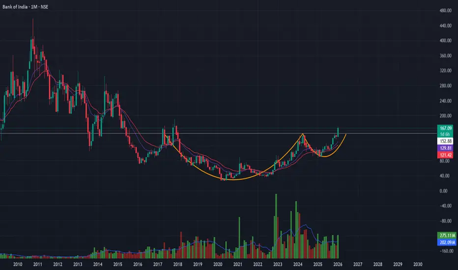
Bank of India | Cup & Handle Breakout SetupStructure:
Long-term Cup & Handle pattern nearing completion on monthly timeframe, indicating accumulation after a prolonged base.
Confirmation Signals:
-Volume expanding on rallies
-RSI above 50 and rising
-OBV trending higher → accumulation visible
-Price holding above short-term EMAs
Trade Plan:
-Buy: Sustained breakout above ₹151
-Targets: ₹199 → ₹268
-Stop-loss: ₹134 (ATR-based, structure-valid)
-Risk–Reward: ~1:5
USD/JPY Intraday Short – Liquidity Sweep & Shift in Market STRFollowing a period of distribution near the 153.750 level, price has shown a clear rejection of recent highs, likely sweeping buy-side liquidity (BSL) before breaking lower.

IRFC 1 Day View 📊 Daily Pivot Levels (1-Day TF)
Pivot (daily equilibrium): ~ ₹115.3 – bias above this = short-term bullish; below = bearish.
📈 Resistance Levels (Upside)
R1: ~ ₹117.0–₹117.1 — first daily resistance.
R2: ~ ₹119.9–₹120.0 — secondary resistance zone.
R3: ~ ₹121.6–₹122.0+ — stronger upside barrier.
📉 Support Levels (Downside)
S1: ~ ₹112.5–₹112.6 — first support around recent lows.
S2: ~ ₹110.8–₹111.0 — next support zone below.
S3: ~ ₹107.9–₹108.0 — deeper support zone from pivot analysis.
🔁 Technical Bias Notes (Daily Timeframe)
Current daily RSI and momentum indicators show bearish to neutral bias, with price often trading below short-term moving averages — sellers have slight edge unless price clears key resistances.
Stochastic and oscillators have shown oversold pressures at times, so short-term bounce near support zones (₹110–₹112) is possible if momentum shifts.

Nifty Realty - An Ignored HIDDEN GEM at solid Risk RewardThis is a ratio chart of Nifty Realty compared to NSE 500
A classic cup formation is being seen on multi year level where nifty realty is in a rising channel formation making higher lows for past 2-3 times since covid
Right now index has taken support again at channel low and reversal looks likely
A series of higher lows, increasing volumes, rising channel and a cup formation all together indicate good solid bullishness on real estate stocks outperforming cnx 500.

NIFTY TREND UPDATIONIn Nifty options trading, a significant increase in Put Open Interest (OI) is a double-edged sword that requires careful technical confirmation. From the perspective of "Smart Money" (option writers), rising Put OI generally builds a floor of Support, as institutional sellers are betting the index will stay above that level to collect premiums. However, your observation is correct: if Nifty is trading near a resistance zone or a trendline, an increase in Put OI alone does not automatically reflect positive strength.
If the index breaks below its established trendlines despite the rising Put OI, it often triggers a "Long Unwinding" or a "Short Buildup" scenario. In this case, Put sellers who were providing support are forced to cover their positions to limit losses, which creates a cascade of selling pressure, leading to a sharp fall. Conversely, if Nifty holds above resistance while Put OI climbs, it confirms that the "floor" is moving higher, potentially leading to a breakout. Without a clear move above resistance, however, the heavy Put OI might simply indicate aggressive hedging or a range-bound market rather than true bullish momentum. Always look for price action to lead the way; OI only tells you where the bets are placed, not which side will eventually win.
