Sector Rotation Strategies1. Introduction to Sector Rotation
In the financial markets, sector rotation is the strategic shifting of investments between different sectors of the economy to capitalize on the varying performance of those sectors during different phases of the economic and market cycle.
The basic premise:
Not all sectors perform equally at the same time.
Economic cycles influence which sectors thrive and which lag.
By positioning capital into the right sectors at the right time, an investor can potentially outperform the overall market.
In practice, sector rotation is a top-down investment approach, starting from macroeconomic conditions → to market cycles → to sector performance → to specific stock selection.
2. Understanding Sectors and Market Cycles
The stock market is divided into 11 primary sectors as classified by the Global Industry Classification Standard (GICS):
Energy – Oil, gas, and related services.
Materials – Mining, chemicals, paper, etc.
Industrials – Manufacturing, aerospace, transportation.
Consumer Discretionary – Retail, luxury goods, entertainment.
Consumer Staples – Food, beverages, household goods.
Healthcare – Pharmaceuticals, biotech, hospitals.
Financials – Banks, insurance, asset managers.
Information Technology (IT) – Software, hardware, semiconductors.
Communication Services – Media, telecom.
Utilities – Electricity, water, gas distribution.
Real Estate – REITs and property developers.
These sectors do not rise and fall together. Instead, they rotate in leadership depending on the stage of the economic cycle.
3. The Economic Cycle and Sector Performance
Sector rotation is deeply connected to the business cycle, which has four broad phases:
Early Expansion (Recovery)
Economy rebounds from a recession.
Interest rates are low, liquidity is high.
Consumer spending begins to rise.
Corporate profits improve.
Leading Sectors: Technology, Consumer Discretionary, Financials.
Mid Expansion (Growth)
Strong GDP growth.
Employment levels are high.
Corporate earnings peak.
Leading Sectors: Industrials, Materials, Energy (as demand rises).
Late Expansion (Peak)
Inflation pressures build.
Central banks raise interest rates.
Growth slows.
Leading Sectors: Energy (inflation hedge), Materials, Consumer Staples, Healthcare.
Contraction (Recession)
GDP falls, unemployment rises.
Consumer spending drops.
Risk assets underperform.
Leading Sectors: Utilities, Consumer Staples, Healthcare (defensive sectors).
Sector Rotation Map
Economic Phase Best Performing Sectors Reason
Early Recovery Tech, Financials, Consumer Discretionary Low rates boost growth stocks
Mid Expansion Industrials, Materials, Energy Demand and capital spending rise
Late Expansion Energy, Materials, Healthcare, Staples Inflation hedging, defensive
Recession Utilities, Consumer Staples, Healthcare Stable cash flows, essential goods
4. Sector Rotation Strategies in Practice
There are two main approaches:
A. Tactical Sector Rotation
Short- to medium-term shifts (weeks to months) based on:
Economic data (GDP growth, inflation, interest rates).
Earnings reports and forward guidance.
Market sentiment indicators.
Technical analysis of sector ETFs and indexes.
Example:
If manufacturing PMI is rising → Industrials & Materials may outperform.
B. Strategic Sector Rotation
Long-term positioning (months to years) based on:
Anticipated shifts in the business cycle.
Structural economic changes (e.g., green energy trend, AI boom).
Demographic trends (aging population → Healthcare demand).
Example:
Positioning into renewable energy over the next decade due to global decarbonization policies.
5. Tools & Indicators for Sector Rotation
Sector rotation isn’t guesswork — it relies on economic, technical, and intermarket analysis.
Economic Indicators:
GDP Growth – High GDP growth favors cyclical sectors; low GDP growth favors defensive sectors.
Interest Rates – Rising rates benefit Financials (banks), hurt rate-sensitive sectors like Real Estate.
Inflation Data (CPI, PPI) – High inflation boosts Energy & Materials.
PMI (Purchasing Managers' Index) – Expanding manufacturing favors Industrials & Materials.
Technical Indicators:
Relative Strength (RS) Analysis – Compare sector ETF performance vs. the S&P 500.
Moving Averages – Identify uptrends/downtrends in sector performance.
Relative Rotation Graphs (RRG) – Visual representation of sector momentum & relative strength.
Market Sentiment Indicators:
Fear & Greed Index – Helps gauge if market is risk-on (cyclicals lead) or risk-off (defensives lead).
VIX (Volatility Index) – High VIX favors defensive sectors.
6. Sector Rotation Using ETFs
The easiest way to implement sector rotation is via sector ETFs.
In the U.S., SPDR offers Select Sector SPDR ETFs:
Sector ETF Ticker
Communication Services XLC
Consumer Discretionary XLY
Consumer Staples XLP
Energy XLE
Financials XLF
Healthcare XLV
Industrials XLI
Materials XLB
Real Estate XLRE
Technology XLK
Utilities XLU
Example Strategy:
Track the top 3 ETFs with the strongest relative strength vs. the S&P 500.
Allocate more capital to them while reducing exposure to underperforming sectors.
Rebalance monthly or quarterly.
7. Historical Examples of Sector Rotation
Example 1 – Post-2008 Recovery
Early 2009: Financials, Tech, Consumer Discretionary surged as markets rebounded from the GFC.
Late 2010–2011: Industrials & Energy took leadership as global growth accelerated.
2012 slowdown: Defensive sectors like Utilities & Healthcare outperformed.
Example 2 – COVID-19 Pandemic
Early 2020 Crash: Utilities, Healthcare, and Consumer Staples outperformed during the panic.
Mid-2020: Tech & Communication Services surged due to remote work and digital adoption.
2021: Energy & Financials surged as the economy reopened and inflation rose.
8. Risks & Challenges in Sector Rotation
While powerful, sector rotation isn’t foolproof.
Challenges:
Timing Risk – Predicting exact cycle turns is hard.
False Signals – Economic indicators can give misleading short-term trends.
Overtrading – Too frequent switching increases costs.
Global Factors – Geopolitics, pandemics, or commodity shocks can disrupt cycles.
Correlation Shifts – Sectors can behave differently than historical patterns.
Example:
In 2023, high interest rates were expected to benefit Financials, but bank failures (SVB collapse) caused underperformance despite the macro setup.
Conclusion
Sector rotation strategies work because capital naturally moves to where growth and safety are perceived.
By understanding:
The economic cycle
Sector behavior in each phase
The right tools & indicators
…investors can align portfolios with the strongest parts of the market at any given time.
However, the strategy requires discipline, patience, and flexibility.
Market cycles can be irregular, and exogenous shocks can disrupt historical patterns. Therefore, sector rotation works best when blended with risk management, diversification, and constant monitoring.
Trade
Algorithmic trading 1. Introduction to Algorithmic Trading
Algorithmic trading, often called algo trading or automated trading, is the process of using computer programs to execute trades in financial markets according to a predefined set of rules.
These rules can be based on price, volume, timing, market conditions, or mathematical models. Once set, the algorithm automatically sends orders to the market without manual intervention.
In simple terms:
Instead of sitting in front of a trading screen and clicking “buy” or “sell,” you tell a machine exactly what conditions to look for, and it trades for you.
It’s like giving your brain + discipline to a computer — minus the coffee breaks, panic, and impulsive decisions.
1.1 Why Algorithms?
Humans are prone to:
Emotional bias (fear, greed, hesitation)
Slow reaction times
Fatigue and inconsistency
Computers, in contrast:
Execute instantly (microseconds or nanoseconds)
Follow rules 100% consistently
Handle multiple markets at once
Backtest ideas over years of data within minutes
This explains why algo trading accounts for 70%–80% of trading volume in developed markets like the US and over 50% in Indian markets for certain instruments.
1.2 The Core Components
Every algorithmic trading system consists of:
Strategy Logic – The rules that trigger trades (e.g., moving average crossover, statistical arbitrage).
Programming Interface – The language/platform (Python, C++, Java, MetaTrader MQL, etc.).
Market Data Feed – Real-time price, volume, and order book data.
Execution Engine – Connects to broker/exchange to place orders.
Risk Management Module – Stops, limits, and capital allocation rules.
Performance Tracker – Monitors profit/loss, drawdowns, and execution quality.
2. How Algorithmic Trading Works – Step by Step
Let’s break it down:
Idea Generation
Define a hypothesis: “I think when the 50-day moving average crosses above the 200-day MA, the stock will trend upward.”
Strategy Design
Turn the idea into exact rules: If MA50 > MA200 → Buy; If MA50 < MA200 → Sell.
Coding the Strategy
Program in Python, C++, R, or a broker’s native scripting language.
Backtesting
Run the algorithm on historical data to see how it would have performed.
Paper Trading (Simulation)
Trade in real time with virtual money to test live conditions.
Execution in Live Markets
Deploy with real money, connected to exchange APIs.
Monitoring & Optimization
Adjust based on performance, slippage, and market changes.
2.1 Example of a Simple Algorithm
Pseudocode:
sql
Copy
Edit
If Close Price today > 20-day Moving Average:
Buy 10 units
If Close Price today < 20-day Moving Average:
Sell all units
The computer checks the rule every day (or every minute, or millisecond, depending on design).
3. Types of Algorithmic Trading Strategies
Algo trading is not one-size-fits-all. Traders and funds design algorithms based on their objectives, timeframes, and risk appetite.
3.1 Trend-Following Strategies
Logic: “The trend is your friend.”
Tools: Moving Averages, MACD, Donchian Channels.
Example: Buy when short-term average crosses above long-term average.
Pros: Simple, works in trending markets.
Cons: Suffers in sideways/choppy markets.
3.2 Mean Reversion Strategies
Logic: Prices eventually revert to their mean (average).
Tools: Bollinger Bands, RSI, z-score.
Example: If stock falls 2% below its 20-day average, buy expecting a bounce.
Pros: Works well in range-bound markets.
Cons: Can blow up if the “mean” shifts due to fundamental changes.
3.3 Statistical Arbitrage
Logic: Exploit price inefficiencies between correlated assets.
Example: If Reliance and TCS usually move together but Reliance lags by 1%, buy Reliance and short TCS expecting convergence.
Pros: Market-neutral, less affected by overall market trend.
Cons: Requires high-frequency execution and deep statistical modeling.
3.4 Market-Making Algorithms
Logic: Provide liquidity by continuously posting buy and sell quotes.
Goal: Earn the bid-ask spread repeatedly.
Risk: Adverse selection during sharp market moves.
3.5 Momentum Strategies
Logic: Stocks that move strongly in one direction will continue.
Tools: Breakouts, Volume Surges.
Example: Buy when price breaks a 50-day high with high volume.
3.6 High-Frequency Trading (HFT)
Executes in microseconds.
Focuses on ultra-short-term inefficiencies.
Requires co-location servers near exchanges for speed advantage.
3.7 Event-Driven Algorithms
React to corporate actions or news:
Earnings releases
Mergers & acquisitions
Dividend announcements
Often combined with natural language processing (NLP) to scan news feeds.
4. Technologies Behind Algo Trading
4.1 Programming Languages
Python – Most popular for beginners & research.
C++ – Preferred for HFT due to speed.
Java – Stable for large trading systems.
R – Strong in statistical modeling.
4.2 Data
Historical Data – For backtesting.
Real-Time Data – For live execution.
Level 2/Order Book Data – For order flow analysis.
4.3 APIs & Broker Platforms
REST APIs – Easy to use but slightly slower.
WebSocket APIs – Low latency, real-time streaming.
FIX Protocol – Industry standard for institutional trading.
4.4 Infrastructure
Cloud Hosting – AWS, Google Cloud.
Dedicated Servers – For low latency.
Co-location – Servers physically near exchange data centers.
5. Advantages of Algorithmic Trading
Speed – Executes in microseconds.
Accuracy – Removes manual entry errors.
Backtesting – Test before risking real money.
Consistency – No emotional bias.
Multi-Market Trading – Monitor dozens of assets simultaneously.
Scalability – Once built, can trade large portfolios.
6. Risks & Challenges in Algo Trading
6.1 Market Risks
Model Overfitting: Works perfectly on past data but fails live.
Regime Changes: Strategies die when market structure shifts.
6.2 Technical Risks
Connectivity Issues
Data Feed Errors
Exchange Downtime
6.3 Execution Risks
Slippage – Orders filled at worse prices due to latency.
Front Running – Competitors' algorithms act faster.
6.4 Regulatory Risks
Many countries have strict algo trading regulations:
SEBI in India requires pre-approval for certain algos.
SEC & FINRA in the US enforce strict monitoring.
7. Backtesting & Optimization
7.1 Steps for Backtesting
Choose historical data range.
Apply your strategy rules.
Measure key metrics:
CAGR (Compound Annual Growth Rate)
Sharpe Ratio
Max Drawdown
Win/Loss Ratio
7.2 Common Pitfalls
Look-Ahead Bias: Using future data unknowingly.
Survivorship Bias: Ignoring stocks that delisted.
Over-Optimization: Tweaking too much to fit past data.
8. Case Study – Moving Average Crossover Algo
Imagine we test a 50-day vs 200-day MA crossover strategy on NIFTY 50 from 2010–2025.
Capital: ₹10,00,000
Buy Rule: MA50 > MA200 → Buy
Sell Rule: MA50 < MA200 → Sell
Results:
CAGR: 11.2%
Max Drawdown: 18%
Trades: 42 over 15 years
Win Rate: 57%
Conclusion: Low trading frequency, steady returns, low drawdown — suitable for positional traders.
Final Thoughts
Algorithmic trading is not a magic money machine — it’s a discipline that combines mathematics, programming, and market knowledge.
When done right, it can offer speed, precision, and scalability far beyond human capability.
When done wrong, it can cause lightning-fast losses.
The game has evolved from shouting in the trading pit to coding in Python. The traders who adapt, learn, and innovate will keep winning — whether they sit in a Wall Street skyscraper or a small home office in Mumbai.
Options Trading Strategies 1. Introduction to Options Trading Strategies
Options are like the “Swiss army knife” of the financial markets — flexible tools that can be shaped to fit bullish, bearish, neutral, or volatile market views. They’re contracts that give you the right, but not the obligation, to buy or sell an asset at a specific price (strike) on or before a certain date (expiry).
While most beginners think options are just for making huge leveraged bets, seasoned traders use strategies — combinations of buying and selling calls and puts — to control risk, generate income, or hedge portfolios.
2. Why Use Strategies Instead of Simple Buy/Sell?
Risk Management: You can cap your losses while keeping upside potential.
Income Generation: Strategies like covered calls and credit spreads generate consistent cash flow.
Direction Neutrality: You can profit even when the market moves sideways.
Volatility Play: You can design trades to profit from expected volatility spikes or drops.
Hedging: Protect stock holdings against adverse moves.
3. The Four Building Blocks of All Strategies
Every complex strategy is built using these four basic positions:
Type Action View Risk Reward
Long Call Buy Bullish Premium Unlimited
Short Call Sell Bearish Unlimited Premium
Long Put Buy Bearish Premium High (to zero)
Short Put Sell Bullish High (to zero) Premium
Once you understand these, combining them is like mixing ingredients to cook different recipes.
4. Categories of Options Strategies
Directional Strategies – Profit from a clear bullish or bearish bias.
Neutral Strategies – Profit from time decay or volatility drops.
Volatility-Based Strategies – Profit from big moves or volatility increases.
Hedging Strategies – Reduce risk on existing positions.
5. Directional Strategies
5.1. Bullish Strategies
These make money when the underlying price rises.
5.1.1 Long Call
Setup: Buy 1 Call
When to Use: Expect sharp upside.
Risk: Limited to premium paid.
Reward: Unlimited.
Example: Nifty at 22,000, buy 22,200 Call for ₹150. If Nifty rises to 22,500, option might be worth ₹300+, doubling your investment.
5.1.2 Bull Call Spread
Setup: Buy 1 ITM/ATM Call + Sell 1 higher strike Call.
Purpose: Lower cost vs. long call.
Risk: Limited to net premium paid.
Reward: Limited to difference between strikes minus premium.
Example: Buy 22,000 Call for ₹200, Sell 22,500 Call for ₹80 → Net cost ₹120. Max profit ₹380 (if Nifty at or above 22,500).
5.1.3 Bull Put Spread (Credit Spread)
Setup: Sell 1 higher strike Put + Buy 1 lower strike Put.
Purpose: Earn premium in bullish to neutral markets.
Risk: Limited to spread width minus premium.
Example: Sell 22,000 Put ₹200, Buy 21,800 Put ₹100 → Credit ₹100.
5.2 Bearish Strategies
These make money when the underlying price falls.
5.2.1 Long Put
Setup: Buy 1 Put.
When to Use: Expect sharp downside.
Risk: Limited to premium paid.
Reward: Large, until stock hits zero.
5.2.2 Bear Put Spread
Setup: Buy 1 higher strike Put + Sell 1 lower strike Put.
Purpose: Cheaper than long put, defined profit range.
Example: Buy 22,000 Put ₹180, Sell 21,800 Put ₹90 → Cost ₹90, Max profit ₹110.
5.2.3 Bear Call Spread
Setup: Sell 1 lower strike Call + Buy 1 higher strike Call.
Purpose: Profit from flat or falling markets.
Example: Sell 22,000 Call ₹250, Buy 22,200 Call ₹150 → Credit ₹100.
6. Neutral Strategies (Time Decay Focus)
These aim to profit if the underlying price stays within a range.
6.1 Iron Condor
Setup: Combine bull put spread and bear call spread.
Goal: Earn premium in range-bound market.
Example: Nifty 22,000 — Sell 21,800 Put, Buy 21,600 Put, Sell 22,200 Call, Buy 22,400 Call.
6.2 Iron Butterfly
Setup: Sell ATM call & put, buy OTM call & put.
Goal: Higher reward, but smaller profit range.
6.3 Short Straddle
Setup: Sell ATM call & put.
Goal: Collect max premium if price stays at strike.
Risk: Unlimited both sides.
6.4 Short Strangle
Setup: Sell OTM call & put.
Goal: Lower premium but wider safety zone.
7. Volatility-Based Strategies
These profit from big moves or volatility changes.
7.1 Long Straddle
Setup: Buy ATM call & put.
Goal: Profit if price moves big in either direction.
When to Use: Pre-event (earnings, budget).
Risk: Premium paid.
7.2 Long Strangle
Setup: Buy OTM call & put.
Cheaper than straddle, needs bigger move.
7.3 Calendar Spread
Setup: Sell near-term option, buy longer-term option (same strike).
Goal: Profit from time decay in short leg & volatility rise.
7.4 Ratio Spreads
Setup: Buy one option, sell more of same type further OTM.
Goal: Take advantage of moderate moves.
8. Hedging Strategies
These protect existing positions.
8.1 Protective Put
Hold stock + Buy Put.
Acts like insurance against downside.
8.2 Covered Call
Hold stock + Sell Call.
Generate income while capping upside.
8.3 Collar
Hold stock + Buy Put + Sell Call.
Limits both upside and downside.
Conclusion
Options trading strategies are not about gambling — they are risk engineering tools. Whether you aim to hedge, speculate, or earn income, you can design a strategy tailored to market conditions. The key is understanding your market view, volatility environment, and risk appetite — and then matching it with the right combination of calls and puts.
Mastering them is like mastering chess: the rules are simple, but winning requires foresight, discipline, and adaptability.
Part11 Trading Masterclass How Options Work
Let’s break this down with an example.
Call Option Example:
You buy a call option on Stock A with a strike price of ₹100, paying a premium of ₹5. If the stock price rises to ₹120, you can buy it for ₹100 and sell it for ₹120—earning a ₹20 profit per share, minus the ₹5 premium, netting ₹15.
If the stock stays below ₹100, you simply let the option expire. Your loss is limited to the ₹5 premium.
Put Option Example:
You buy a put option on Stock A with a strike price of ₹100, paying a ₹5 premium. If the stock falls to ₹80, you can sell it for ₹100—earning ₹20, minus ₹5 premium = ₹15 profit.
If the stock stays above ₹100, the option expires worthless. Again, your loss is limited to ₹5.
Why Trade Options?
A. Leverage
Options require a smaller initial investment compared to buying stocks, but they can offer significant returns.
B. Risk Management (Hedging)
Options can hedge against downside risk. For example, if you own shares, buying a put option can protect you against losses if the price falls.
C. Income Generation
Writing (selling) options like covered calls can generate consistent income.
D. Strategic Flexibility
You can profit in bullish, bearish, or neutral markets using different strategies.

Part11 Trading MasterclassTypes of Option Traders
1. Speculators
They aim to profit from market direction using options. Their goal is capital gain.
2. Hedgers
They use options to protect investments from unfavorable price movements.
3. Income Traders
They sell options to earn premium income.
Option Trading Strategies
1. Basic Strategies
A. Buying Calls (Bullish)
Used when you expect the stock to rise.
B. Buying Puts (Bearish)
Used when expecting a stock to fall.
C. Covered Call (Neutral to Bullish)
Own the stock and sell a call option. Earn premium while holding the stock.
D. Protective Put (Insurance)
Own the stock and buy a put option to limit losses.
2. Intermediate Strategies
A. Vertical Spreads
Buying and selling options of the same type (call or put) with different strike prices.
Bull Call Spread: Buy a lower strike call, sell a higher strike call.
Bear Put Spread: Buy a higher strike put, sell a lower strike put.
B. Iron Condor (Neutral)
Sell OTM put and call options, buy further OTM put and call to limit risk. Profit if the stock stays within a range.
C. Straddle (Volatility)
Buy a call and a put at the same strike price. Profits from big price movement in either direction.

Part9 Trading MasterclassHow Options Work
Let’s break this down with an example.
Call Option Example:
You buy a call option on Stock A with a strike price of ₹100, paying a premium of ₹5. If the stock price rises to ₹120, you can buy it for ₹100 and sell it for ₹120—earning a ₹20 profit per share, minus the ₹5 premium, netting ₹15.
If the stock stays below ₹100, you simply let the option expire. Your loss is limited to the ₹5 premium.
Put Option Example:
You buy a put option on Stock A with a strike price of ₹100, paying a ₹5 premium. If the stock falls to ₹80, you can sell it for ₹100—earning ₹20, minus ₹5 premium = ₹15 profit.
If the stock stays above ₹100, the option expires worthless. Again, your loss is limited to ₹5.
Why Trade Options?
A. Leverage
Options require a smaller initial investment compared to buying stocks, but they can offer significant returns.
B. Risk Management (Hedging)
Options can hedge against downside risk. For example, if you own shares, buying a put option can protect you against losses if the price falls.
C. Income Generation
Writing (selling) options like covered calls can generate consistent income.
D. Strategic Flexibility
You can profit in bullish, bearish, or neutral markets using different strategies.

Retail vs Institutional Trading Introduction
The stock market serves as a vast arena where two primary participants operate — retail traders and institutional traders. Both these groups play crucial roles in the financial ecosystem but differ drastically in terms of capital, strategies, access to information, and influence on the market.
Understanding the dynamics between retail and institutional trading is vital for any market participant — whether you're an investor, trader, analyst, or policymaker. This in-depth analysis unpacks the core differences, strategies, advantages, disadvantages, and market impact of both retail and institutional traders.
1. Definition and Key Characteristics
Retail Traders
Retail traders are individual investors who trade in their personal capacity, usually through online brokerage accounts. They use their own capital and typically trade in smaller volumes.
Key characteristics of retail traders:
Trade small positions (1–1000 shares)
Use online brokerages like Zerodha, Robinhood, or E*TRADE
Rely on public news, retail-focused tools, and charts
Often influenced by social media and sentiment
Usually part-time or hobbyist traders
Institutional Traders
Institutional traders trade on behalf of large organizations, such as:
Mutual funds
Hedge funds
Pension funds
Insurance companies
Sovereign wealth funds
Banks and proprietary trading firms
Key characteristics:
Trade large blocks (10,000+ shares)
Access to sophisticated tools, real-time data, and dark pools
Employ quantitative models and professional teams
Long-term investment strategies or high-frequency trading
Can move markets with a single trade
2. Access to Information & Tools
Retail Access
Retail traders are usually last in line when it comes to access:
Get news after it's public
Use delayed or less granular market data
Basic tools (e.g., TradingView, MetaTrader, ThinkOrSwim)
May rely on YouTube, Twitter, Reddit (e.g., r/WallStreetBets)
Institutional Access
Institutions enjoy early and exclusive access:
Bloomberg Terminal, Reuters Eikon, proprietary feeds
Real-time Level II and III market data
Insider connections (e.g., earnings calls, conferences)
AI-powered data analytics and algorithmic models
Conclusion: Institutional traders operate with a significant information edge.
3. Capital and Buying Power
Retail Traders
Typically operate with limited capital — from ₹10,000 to ₹10 lakhs (or more)
Use margin cautiously due to high risks and interest costs
Constrained by capital preservation and risk tolerance
Institutional Traders
Manage hundreds of crores to billions in assets
Use prime brokerages for margin, shorting, and leverage
Can influence market pricing and supply-demand dynamics
Conclusion: Institutions have a massive capital advantage, enabling economies of scale.
4. Market Impact
Retail Traders’ Impact
Minimal direct impact on prices individually
Collectively can drive momentum trades or short squeezes (e.g., GameStop, Adani stocks)
More reactionary than proactive
Institutional Traders’ Impact
Can shift entire sectors or indices with a single reallocation
Often deploy block trades, iceberg orders, and dark pools to mask intent
Central to price discovery and volume
Conclusion: Institutional flow is the dominant force in price action, while retail adds volatility and liquidity.
5. Trading Strategies
Retail Traders' Strategies
Retail traders typically rely on:
Technical Analysis: Candlesticks, RSI, MACD, chart patterns
Swing Trading / Intraday
News-based or Sentiment-based Trading
Options trading with small lots
Copy trading or Telegram tips (not recommended)
Behavioral tendencies:
Fear of missing out (FOMO)
Overtrading
Chasing breakouts or rumors
Institutional Strategies
Institutions use more structured approaches:
Fundamental Analysis: DCF, macro trends, earnings forecasts
Quantitative Trading: Algorithms, statistical arbitrage
Hedging & Risk Modeling
Portfolio Diversification & Rebalancing
High-Frequency Trading (HFT)
Behavioral tendencies:
Discipline over emotion
Regulatory compliance
Portfolio-level thinking, not trade-by-trade
Conclusion: Retail strategies are shorter-term and emotional, while institutional strategies are data-driven and systematic.
6. Cost of Trading
Retail Traders
Pay higher brokerage fees (especially in traditional full-service brokers)
Have wider bid-ask spreads
Face slippage during volatile moves
No access to negotiated commissions
Institutional Traders
Enjoy preferential fee structures
Access lower spreads via direct market access (DMA)
Use smart order routing to reduce costs
May participate in dark pools to hide trade intent
Conclusion: Institutions enjoy cheaper and more efficient execution.
7. Emotional vs Rational Decision-Making
Retail Traders
Highly influenced by emotions: greed, fear, hope
Overreact to headlines and rumors
Lack discipline and trade management
Often trade without stop-loss
Institutional Traders
Decision-making is systematic and risk-managed
Operate with clear mandates, risk teams, and drawdown controls
Use quantitative models to remove human error
Conclusion: Institutions are generally rational and rule-based, while retail is often impulsive.
8. Regulations and Restrictions
Retail Traders
Face basic regulations (e.g., KYC, margin limits)
No oversight in strategy or risk exposure
Limited access to instruments (e.g., no direct access to foreign derivatives or institutional debt)
Institutional Traders
Heavily regulated by bodies like SEBI, RBI, SEC, etc.
Must follow:
Disclosure norms
Risk-based capital adequacy
Audit and compliance checks
Subject to insider trading laws, fiduciary responsibilities
Conclusion: Retail is freer but riskier, institutional is compliant but structured.
9. Education and Skill Levels
Retail Traders
Largely self-taught
Learn via:
YouTube, Udemy, Twitter
Paid telegram groups, mentors
Often lack deep financial literacy
Institutional Traders
Often have backgrounds in:
Finance, Economics, Math, Computer Science
MBAs, CFAs, PhDs
Supported by quant teams, analysts, economists
Conclusion: Institutional traders have stronger academic and experiential grounding.
10. Time Horizon and Holding Period
Retail Traders
Mostly short-term focused: scalping, intraday, swing
Rarely think in portfolio terms
Less concerned with long-term CAGR
Institutional Traders
Long-term focused (mutual funds, pension funds)
Hedge funds may have medium-term or tactical outlook
Often look at multi-year trends, sector rotation, macro cycles
Conclusion: Retail thinks in days or weeks, institutions think in years.
Conclusion
The divide between retail and institutional traders is significant but narrowing. While institutions dominate in terms of capital, technology, and influence, retail traders now have unprecedented access to tools and knowledge.
For success in modern markets:
Retail traders must focus on discipline, risk, and learning
Institutional players must remain agile and avoid herd behavior
Both groups are vital to the health and vibrancy of the financial markets. Understanding the strengths and limitations of each helps investors better navigate today’s complex market landscape.
Global Factors & Commodities Impact Introduction
In today’s hyperconnected world, no market or economy functions in isolation. Global factors—from geopolitics to central bank decisions—exert profound influence on economies, financial markets, currencies, and especially commodities. Commodities, being the raw backbone of industrial production and human consumption, respond swiftly and often dramatically to global shifts.
Understanding the interplay between global factors and commodity prices is essential for traders, investors, policymakers, and analysts alike. This document presents a detailed exploration of how key global dynamics affect commodities and how in turn, those commodities shape macroeconomic and financial landscapes.
I. Understanding Commodities and Their Role
Commodities are basic goods used in commerce, interchangeable with other goods of the same type. These are broadly categorized into:
Hard Commodities: Natural resources like oil, gas, gold, copper.
Soft Commodities: Agricultural products like wheat, coffee, sugar, cotton.
Commodities as Economic Indicators
Barometers of economic health: Rising industrial metals like copper signal strong manufacturing, while falling oil prices may suggest a slowdown.
Safe-haven assets: Gold typically rallies during geopolitical tension or financial instability.
Inflation hedges: Commodities often rise in inflationary periods as raw material costs increase.
II. Key Global Factors Influencing Commodities
Let’s explore the major global macro factors and how they influence the commodities market:
1. Geopolitical Events
a) War, Tensions, and Conflict
Wars in resource-rich regions (e.g., Middle East) disrupt oil supply, causing prices to spike.
Tensions in Eastern Europe (like the Russia-Ukraine war) impacted natural gas, wheat, and fertilizer prices.
b) Sanctions and Trade Restrictions
US sanctions on Iran or Russia impact global energy flows.
Export bans (e.g., Indonesia on palm oil, India on wheat) cause global supply shortages.
2. Monetary Policy & Central Banks
a) US Federal Reserve Policy
Fed rate hikes strengthen the dollar, making commodities (priced in USD) more expensive globally, which suppresses demand and prices.
Lower interest rates can spur commodity demand due to cheaper credit.
b) Global Liquidity and Inflation
High global liquidity often leads to speculative inflows in commodities.
Inflation leads to increased interest in commodities as an inflation hedge (e.g., gold, oil).
3. US Dollar Index (DXY)
Commodities are dollar-denominated:
Stronger USD = commodities become costlier for foreign buyers → demand drops → prices fall.
Weaker USD = makes commodities cheaper globally → boosts demand → prices rise.
There’s a strong inverse correlation between DXY and commodities like crude oil, copper, and gold.
4. Global Economic Growth & Recession
a) Growth Phases
Industrial growth in China or India boosts demand for base metals (copper, zinc).
Infrastructure development increases demand for energy and materials.
b) Recessionary Trends
Slowdowns cause demand to collapse, reducing prices.
Oil prices fell sharply during COVID-19-induced global lockdowns.
5. Climate and Weather Patterns
a) Natural Disasters & Droughts
Hurricanes in the Gulf of Mexico disrupt oil production.
Droughts in Brazil affect coffee and sugar output.
b) El Niño / La Niña
These cyclical weather patterns alter rainfall and crop yields globally, heavily affecting soft commodities.
6. Technological Changes & Energy Transition
Green energy transition increases demand for lithium, cobalt, nickel (used in EV batteries).
Decline in fossil fuel investments can lead to long-term supply constraints even as demand persists.
7. Global Supply Chains & Shipping
Port congestion, container shortages, or shipping route blockades (e.g., Suez Canal) raise transportation costs and delay supply of commodities.
COVID-19 and its aftermath heavily disrupted supply chains, affecting availability and prices of everything from semiconductors to steel.
8. Speculation & Financialization
Hedge funds and institutional investors increasingly use commodity futures for diversification or speculation.
Large inflows into commodity ETFs can drive prices independent of actual supply-demand fundamentals.
III. Case Studies: How Global Factors Moved Commodity Markets
Case Study 1: Russia-Ukraine War (2022–2023)
Crude Oil: Brent soared above $130/bbl due to fear of Russian supply disruptions.
Natural Gas: European gas prices skyrocketed due to dependency on Russian pipelines.
Wheat & Corn: Ukraine, being a global grain exporter, saw blocked exports, leading to food inflation globally.
Fertilizers: Russia is a major potash exporter; sanctions caused fertilizer shortages and global agricultural stress.
Case Study 2: COVID-19 Pandemic (2020)
Oil Collapse: WTI futures turned negative in April 2020 due to oversupply and zero demand.
Gold Rally: Fears of economic collapse, stimulus packages, and inflation boosted gold past $2000/oz.
Copper and Industrial Metals: After initial crash, recovery driven by Chinese infrastructure stimulus boosted prices.
Case Study 3: China's Economic Boom (2000s–2010s)
China’s meteoric growth led to a commodity supercycle.
Demand from real estate and infrastructure drove up prices of:
Iron ore
Copper
Coal
Oil
Global mining and metal exporting nations like Australia, Brazil, and South Africa benefited immensely.
IV. Commodities’ Feedback on the Global Economy
Just as global events influence commodities, the price and availability of commodities influence the global economy:
1. Inflation Driver
High commodity prices lead to cost-push inflation.
Example: Crude oil spikes increase transportation, manufacturing, and plastic costs.
2. Trade Balance Impacts
Commodity-importing nations (like India for oil) suffer higher deficits when prices rise.
Exporters (like Saudi Arabia, Australia) benefit from higher revenue and forex reserves.
3. Interest Rate Policy
Central banks may hike rates to control inflation caused by commodity spikes.
Commodity-driven inflation can trigger stagflation, forcing tough monetary decisions.
4. Consumer Spending
Fuel and food price inflation reduces disposable income, hurting demand for discretionary goods.
5. Corporate Profit Margins
Industries reliant on raw materials (FMCG, auto, infrastructure) face margin pressure with rising input costs.
V. Sector-Wise Impact of Commodities
1. Energy Sector
Oil & Gas companies benefit from rising crude prices.
Refining margins and exploration investments become attractive.
2. Metals & Mining
Companies like Vedanta, Hindalco benefit from higher prices of aluminum, copper, etc.
Steel sector tracks iron ore and coking coal prices.
3. Agriculture
Fertilizer, sugar, edible oil, and agrochemical companies see profits swing with crop and soft commodity trends.
4. Transportation and Logistics
High fuel prices hurt airlines, shipping, and logistics firms.
Global supply bottlenecks also affect these industries directly.
VI. Key Commodities and Their Global Sensitivities
1. Crude Oil
Prone to OPEC decisions, Middle East tensions, US shale output.
Benchmark for energy inflation.
2. Gold
Sensitive to interest rates, dollar strength, and geopolitical tension.
Hedge against currency devaluation and inflation.
3. Copper
Dubbed “Doctor Copper” due to its predictive power for global growth.
Used extensively in construction, electronics, EVs.
4. Natural Gas
Seasonal demand (winter heating), pipeline issues, and storage levels dictate prices.
LNG is reshaping global gas trade patterns.
5. Wheat, Corn, and Soybeans
Affected by droughts, wars, and export policies.
Also influenced by biofuel policies (e.g., corn for ethanol).
6. Lithium, Nickel, Cobalt
Critical for battery manufacturing.
Demand surging due to EV and renewable energy expansion.
VII. Emerging Trends in Commodity Markets
1. Green Commodities Boom
Demand for rare earths, lithium, and graphite surging due to energy transition.
2. Decentralized Supply Chains
Countries diversifying supply sources to reduce risk of disruptions (e.g., China+1 strategy).
3. Digital Commodities Platforms
Blockchain and AI-based trading platforms increasing transparency and liquidity in physical commodity markets.
4. ESG Impact
Environmental and social governance (ESG) concerns influencing investment in mining and fossil fuels.
Restrictions on dirty industries affect future supply potential.
VIII. Strategies for Traders & Investors
A. Hedging with Commodities
Institutional investors use commodities to hedge equity, bond, and inflation risks.
B. Trading through Derivatives
Futures, options, and commodity ETFs enable exposure to price movements.
C. Following Macro Themes
Aligning trades with prevailing global trends (e.g., buying lithium during EV boom).
D. Currency-Commodities Interplay
Monitoring USD, INR, and other forex trends for insights into commodity direction.
E. Sentiment & News Monitoring
Quick reactions to breaking geopolitical or economic news can create trading opportunities.
IX. Conclusion
Commodities form the bedrock of the global economy, and their prices act as both signals and triggers for macroeconomic trends. As we've seen, a wide range of global factors—monetary policy, geopolitical events, dollar strength, supply-chain dynamics, and technological shifts—all converge to influence commodity markets.
In turn, the direction of commodities affects everything from inflation and interest rates to corporate profitability and trade balances. Therefore, understanding the interlinked feedback loop between global factors and commodities is essential for anyone navigating the financial world—be it a retail investor, policymaker, fund manager, or trader.
In the era of globalization and real-time information flow, commodities have become not just economic inputs but macroeconomic indicators, capable of shaking up entire industries and shifting the course of national economies. As we move forward into a world shaped by climate change, deglobalization, digital transformation, and geopolitical flux, commodities will remain at the center of global financial narratives.

Part7 Trading Master Class How Options Work
Example of a Call Option
Suppose a stock is trading at ₹100. You buy a call option with a ₹110 strike price, expiring in 1 month, and pay a ₹5 premium.
If the stock rises to ₹120: Your profit is ₹120 - ₹110 = ₹10. Net gain = ₹10 - ₹5 = ₹5.
If the stock stays at ₹100: The option expires worthless. Your loss = ₹5 (premium).
Example of a Put Option
Suppose the same stock is ₹100, and you buy a put option with a ₹90 strike price for ₹5.
If the stock drops to ₹80: Your profit = ₹90 - ₹80 = ₹10. Net gain = ₹10 - ₹5 = ₹5.
If the stock stays above ₹90: The option expires worthless. Your loss = ₹5.
Types of Options
American vs. European Options
American Options: Can be exercised anytime before expiry.
European Options: Can only be exercised at expiry.
Index Options vs. Stock Options
Stock Options: Based on individual stocks (e.g., Reliance, Infosys).
Index Options: Based on indices (e.g., Nifty, Bank Nifty).
Weekly vs. Monthly Options
Weekly Options: Expire every Thursday (India).
Monthly Options: Expire on the last Thursday of the month.

Part3 Learn Institutional Trading Options Trading in India
In India, options are primarily traded on the National Stock Exchange (NSE). Some key features:
Lot Size: Options are traded in fixed lot sizes (e.g., Nifty = 50 units).
Settlement: Cash-settled (no delivery of underlying).
Expiry: Weekly (Thursday) and Monthly (last Thursday).
Margins: Sellers must maintain margin with their broker.
Popular contracts include:
Nifty 50 Options
Bank Nifty Options
Fin Nifty Options
Stock Options (e.g., Reliance, HDFC, TCS)
Tools & Platforms
Successful options trading often relies on good tools:
Broker Platforms: Zerodha, Upstox, Angel One, ICICI Direct.
Charting Tools: TradingView, ChartInk, Fyers.
Option Analysis Tools:
Sensibull
Opstra DefineEdge
QuantsApp
NSE Option Chain
These tools help visualize OI (Open Interest), build strategies, and simulate outcomes.
Taxes on Options Trading (India)
Income Head: Classified under business income.
Tax Rate: Taxed as per income slab or presumptive basis.
Audit: Required if turnover exceeds ₹10 crore or loss is claimed.
GST: Not applicable to retail option traders.
Always consult a CA or tax expert for compliance and accurate filing.
Risk Management in Options
Key rules for managing risk:
Position Sizing: Never risk more than 1–2% of capital per trade.
Diversification: Avoid putting all capital in one strategy.
Stop Losses: Predefined exit points reduce emotional trading.
Avoid Illiquid Contracts: Wider bid-ask spreads hurt profitability.
Avoid Overleveraging: Leverage can magnify both gains and losses.

Part9 Trading Masterclass Psychology of Options Trading
Success in options is 70% psychology and 30% strategy. Key mental traits:
Discipline: Stick to your rules.
Patience: Wait for right setups.
Control Greed/Fear: Avoid revenge trading or FOMO.
Learning Mindset: Options are complex — keep updating your knowledge.
Tips for Beginners
Start with buying options, not writing.
Avoid expiry day trading initially.
Study Open Interest (OI) and Option Chain data.
Use strategy builders before placing real trades.
Maintain a trading journal to review and improve.

Quantitative Trading1. Introduction to Quantitative Trading
Quantitative Trading (or “quant trading”) is the use of mathematical models, statistical techniques, and computational tools to identify and execute trading opportunities in financial markets. It replaces subjective decision-making with rule-based, data-driven strategies.
Instead of relying on "gut feeling" or news events, quant traders trust historical data, patterns, and algorithms. It combines elements of finance, mathematics, programming, and data science to develop systems that can analyze thousands of data points within milliseconds.
2. Evolution of Quantitative Trading
Quantitative trading has grown significantly since the 1980s. Initially confined to hedge funds and institutions like Renaissance Technologies or D. E. Shaw, it is now increasingly accessible due to:
Cheaper computing power
Open-source data libraries
Online brokers with APIs
Educational platforms on Python, R, etc.
Even retail traders can now design and test systematic strategies using tools like QuantConnect, Backtrader, or MetaTrader.
3. Core Components of Quantitative Trading
A. Data
Quant trading is data-centric. Types of data used include:
Market Data: Price, volume, order book
Fundamental Data: P/E ratio, balance sheet figures
Alternative Data: Satellite imagery, sentiment, weather, etc.
Tick-level Data: High-frequency data by milliseconds
B. Alpha Generation
Alpha refers to the edge or profitability of a strategy. Quantitative traders search for alpha using:
Statistical Arbitrage
Mean Reversion
Momentum
Factor Models
Machine Learning Classifiers
They validate alpha through backtesting and cross-validation.
C. Strategy Design
A quant strategy consists of:
Hypothesis: E.g., “Small caps outperform large caps in January”
Signal Generation: Quantifying when to buy or sell
Risk Management: Avoiding large drawdowns
Execution Logic: How trades are placed (market/limit orders)
Performance Metrics: Sharpe ratio, drawdown, win-rate, etc.
D. Backtesting and Simulation
Backtesting simulates a strategy on historical data. Key metrics:
CAGR (Compound Annual Growth Rate)
Maximum Drawdown
Sortino Ratio (downside risk-adjusted return)
Win/Loss ratio
Trade frequency
Robust backtesting avoids overfitting, which leads to poor real-world performance.
E. Execution Algorithms
Execution is critical. Poor fills or slippage can erode profits. Execution strategies include:
VWAP/TWAP (volume/time-weighted average price)
Sniper/iceberg algorithms
Smart Order Routing (SOR)
Latency-sensitive strategies like high-frequency trading (HFT) need co-location with exchanges for microsecond execution.
4. Types of Quantitative Trading Strategies
A. Statistical Arbitrage
Uses statistical relationships between instruments. For example:
Pairs Trading: Buy one stock, short another when their historical spread diverges
Cointegration Models: Mathematically test if two securities move together
B. Mean Reversion
Assumes price deviates from the mean and eventually reverts.
Z-score: Measures how far a price is from the mean
Bollinger Bands: Signal overbought/oversold levels
C. Momentum Strategies
Buy assets that are going up and sell those going down.
Price Momentum: 12-month trailing returns
Relative Strength Index (RSI): Overbought/oversold indicator
Cross-asset Momentum: FX, commodities, equities, etc.
D. Factor-Based Investing
Quantifies characteristics ("factors") that drive returns:
Value: Low P/E, high dividend yield
Size: Small vs. large caps
Quality: Profitability, earnings stability
Low Volatility: Defensive stocks
Momentum: Strong performers
E. High-Frequency Trading (HFT)
Extremely fast, algorithm-driven trading based on:
Order book imbalances
Quote stuffing and spoofing detection
Market microstructure patterns
Requires low latency infrastructure, ultra-fast data feeds, and specialized hardware (e.g., FPGAs).
F. Machine Learning-Based Strategies
Use supervised or unsupervised learning for:
Price prediction
Regime detection
Portfolio optimization
Sentiment analysis
Popular algorithms include Random Forests, XGBoost, SVMs, Neural Networks, and Reinforcement Learning.
5. Quantitative Trading Workflow
Step 1: Idea Generation
Form a hypothesis using theory, observation, or data mining. For example:
"Stocks with increasing earnings surprises tend to outperform"
"Cryptocurrencies follow momentum patterns during news-driven moves"
Step 2: Data Collection
Use data from:
Bloomberg, Quandl, Refinitiv
APIs like Alpha Vantage, Yahoo Finance, Polygon
Alternative providers like RavenPack (news), Orbital Insight (satellite data)
Step 3: Data Cleaning and Processing
Remove:
Missing values
Outliers
Look-ahead bias
Survivorship bias
Normalize features and engineer inputs for the model (e.g., log returns, rolling averages).
Step 4: Backtest and Evaluate
Backtest using realistic constraints:
Bid/ask spread
Slippage
Latency
Transaction costs
Compare in-sample vs. out-of-sample performance.
Step 5: Paper Trading / Forward Testing
Run your strategy live with simulated capital to test its real-time behavior without risking real money.
Step 6: Live Deployment
Integrate with brokers using APIs (e.g., Interactive Brokers, Alpaca, Zerodha Kite Connect).
Set up:
Real-time data feeds
Execution systems
Risk controls (drawdown limits, position limits)
Monitor performance and retrain models if needed.
6. Tools and Languages Used
A. Programming Languages
Python (most common, thanks to libraries like Pandas, NumPy, Scikit-learn, TensorFlow)
R (good for statistical modeling)
C++/Java (for high-performance, low-latency systems)
B. Backtesting Libraries
Backtrader (Python)
QuantConnect (LEAN engine)
Zipline (used by Quantopian)
PyAlgoTrade
C. Broker APIs
Interactive Brokers
Zerodha Kite
TD Ameritrade
Alpaca Markets
D. Data Tools
SQL/NoSQL databases
Jupyter Notebooks for exploratory analysis
Docker/Kubernetes for scalable deployments
AWS/GCP/Azure for cloud-based computation
Conclusion
Quantitative trading represents a paradigm shift in how financial markets are analyzed and traded. By combining math, programming, and finance, quants can find repeatable patterns and automate their exploitation. While complex and resource-intensive, it offers tremendous potential for those who can master its intricacies.
However, it's not a magic bullet. Quant trading requires rigorous testing, constant adaptation, and a deep understanding of markets. Strategies must be robust, scalable, and continuously evaluated to stay ahead in an increasingly crowded and data-driven environment.
For aspiring traders, learning quantitative trading unlocks a world where code and computation meet capital and creativity
Part1 Ride The Big MovesOption Trading Tools & Platforms
Key tools for effective options trading:
Option Chain Analysis Tools (NSE, Sensibull, Opstra, etc.)
Payoff Diagram Simulators
Greeks Calculators
Strategy Builders
Volatility Charts (IV, HV)
Successful Option Trader’s Mindset
The best option traders are not gamblers. They:
Focus on risk management (position sizing, stop loss)
Use strategies, not guesses
Understand Greeks and volatility
Prefer probability over prediction
Learn from every trade
The Future of Options Trading
With tech-driven innovations, we are seeing:
Zero Day Expiry Options (0DTE) gaining popularity
AI-driven options strategies
Increased retail participation through mobile apps
Automated trading using APIs and bots
Micro contracts for better accessibility

Part5 Institutional Trading Why Traders Use Options
Options are not just for speculation—they serve many purposes:
🎯 Speculation
Traders can take directional bets with limited capital.
🛡️ Hedging
Protect your portfolio or a specific stock against adverse movements.
💰 Income Generation
By selling options (covered calls or puts), you can earn premium income.
🎯 Leverage
Control larger exposure with less capital, but with higher risk.
Real-World Example: Call Option
Imagine Reliance stock is at ₹2500.
You buy a Call Option with strike ₹2600, premium ₹50, expiry in 2 weeks.
Scenario A – Price goes to ₹2700:
Profit = (2700 – 2600 – 50) = ₹50 profit per share
ROI = ₹50 / ₹50 = 100%
Scenario B – Price remains ₹2500:
Loss = Full premium = ₹50 (option expires worthless)

Retail Trading vs Institutional TradingIntroduction
The financial markets are a dynamic ecosystem composed of diverse participants ranging from individual investors to large financial institutions. These participants can be broadly categorized into retail traders and institutional traders. While both aim to generate profits from the markets, they operate on fundamentally different scales, use different strategies, and face varying levels of regulation and risk exposure.
This article explores the essential differences between retail and institutional trading, comparing their objectives, tools, advantages, limitations, and market impact. Understanding this distinction is crucial for traders, investors, and market analysts alike.
1. What is Retail Trading?
Retail trading refers to the buying and selling of securities by individual investors who manage their own money. These traders typically use brokerage platforms such as Zerodha, Upstox, Robinhood, or Interactive Brokers to place trades in stocks, bonds, derivatives, mutual funds, and ETFs.
Key Characteristics of Retail Traders:
Trade using personal funds
Use online trading platforms
Typically trade in small volumes
Limited access to advanced tools and research
Often influenced by market sentiment and news
Operate independently
Common Participants:
Individual investors
Self-directed traders
Hobbyists and part-time traders
Beginner investors using mobile apps
2. What is Institutional Trading?
Institutional trading is conducted by large organizations that manage vast amounts of capital on behalf of clients or stakeholders. These include mutual funds, hedge funds, insurance companies, pension funds, investment banks, and proprietary trading firms.
Key Characteristics of Institutional Traders:
Trade large volumes of securities
Use proprietary algorithms and data analytics
Employ teams of analysts, economists, and quants
Can influence market trends due to trade size
Often get better pricing (e.g., lower spreads, negotiated commissions)
Subject to stricter regulatory requirements
Common Participants:
Mutual funds
Hedge funds
Pension funds
Insurance companies
Sovereign wealth funds
Family offices
Asset management firms
3. Core Differences Between Retail and Institutional Trading
Aspect Retail Trading Institutional Trading
Capital Size Small (thousands to lakhs) Large (crores to billions)
Tools & Technology Basic to moderate tools High-end proprietary tools & infrastructure
Access to Information Public and delayed data Real-time data, deep analytics, and research
Trading Costs Higher relative commissions Lower commissions due to bulk discounts
Market Impact Minimal Significant due to trade size
Investment Horizon Short-term to medium-term Varies—can be short, medium, or long-term
Speed & Execution Slower execution High-speed execution using smart order routing
Risk Management Often basic or emotional Systematic with hedging and quantitative models
Regulatory Compliance Limited oversight Extensive regulations and audits
Leverage Availability Limited Significant leverage (with risk controls)
4. Tools & Technologies
Retail Traders:
Trading apps (e.g., Zerodha Kite, Robinhood)
Charting platforms (e.g., TradingView)
Technical indicators (MACD, RSI, Bollinger Bands)
Social media and forums for sentiment analysis
Institutional Traders:
Direct Market Access (DMA)
High-Frequency Trading (HFT) infrastructure
Bloomberg Terminal and Reuters Eikon
Algorithmic trading engines
Risk Management Systems (RMS)
Machine Learning & AI models for prediction
5. Strategies Used
Retail Trading Strategies:
Day Trading: Buying and selling within the same day
Swing Trading: Capturing price swings over a few days
Position Trading: Holding for weeks or months
Momentum Trading: Riding price momentum
Technical Analysis: Relying on chart patterns and indicators
Institutional Trading Strategies:
Arbitrage: Exploiting price differences across markets
Quantitative Models: Using mathematical models to trade
High-Frequency Trading (HFT): Executing thousands of trades per second
Long/Short Equity: Simultaneously buying undervalued and shorting overvalued stocks
Portfolio Hedging: Using options and futures to manage risk
Dark Pool Trading: Executing large trades without impacting the market
6. Advantages & Disadvantages
Retail Trading Advantages:
Flexibility: Can enter and exit positions quickly
No Mandates: No pressure to follow institutional mandates
Wide Choices: Can explore niche assets (e.g., penny stocks, crypto)
Learning Curve: Great platform to learn and experiment
Retail Trading Disadvantages:
Lack of Access: No early access to IPOs or insider pricing
Emotional Decisions: Prone to fear and greed
Higher Costs: Commissions and spreads are relatively higher
Limited Research: Often rely on social media or basic tools
Institutional Trading Advantages:
Deep Research: Backed by teams of analysts and economists
Negotiated Costs: Lower execution costs
Market Access: Access to IPO allocations, block deals, dark pools
Risk Management: Strong systems and frameworks in place
Institutional Trading Disadvantages:
Slower Flexibility: Large trades require strategic execution
Regulatory Burden: Heavily regulated and audited
Crowded Trades: Many institutions follow similar models, leading to herd behavior
7. Regulatory Landscape
Retail Traders:
Must comply with basic market regulations set by authorities like SEBI (India), SEC (USA), or FCA (UK)
Brokers manage KYC/AML compliance
Retail participation is encouraged for market democratization
Institutional Traders:
Face heavy scrutiny and reporting requirements
Subject to detailed disclosures, audits, and risk controls
Must adhere to fund mandates, client transparency norms, and regulatory caps
8. Market Influence
Retail Impact:
Retail traders often move smaller-cap stocks due to low liquidity. However, when acting in mass (e.g., during meme stock frenzies like GameStop in 2021), they can disrupt even large-cap stocks temporarily.
Institutional Impact:
Institutions shape long-term trends. Their decisions impact indices, bond yields, sectoral allocations, and global flows. For example, when FIIs (Foreign Institutional Investors) sell off Indian equities, the market often sees sharp corrections.
9. Case Studies
GameStop (2021) – Retail Power:
A short squeeze initiated by Reddit's r/WallStreetBets community caused GameStop shares to skyrocket, hurting hedge funds and proving that coordinated retail action can temporarily disrupt institutional strategies.
LIC IPO (India 2022) – Institutional Influence:
India’s largest-ever IPO saw massive institutional participation, shaping investor confidence and price discovery even before listing.
10. Risk Profiles
Retail Risks:
Lack of diversification
Overtrading or using excessive leverage
Chasing trends without research
Emotional bias
Institutional Risks:
Portfolio concentration in similar assets
Black swan events affecting large positions
Regulatory or compliance breaches
Liquidity mismatches in stressed times
Conclusion
Retail and institutional trading represent two ends of the financial market spectrum. While institutions control the majority of market volume and influence, retail traders are growing rapidly in number, especially in emerging markets like India.
Each has its strengths and weaknesses. Retail traders enjoy flexibility and personal control but lack the tools and scale of institutions. On the other hand, institutions command influence and resources but face regulatory and structural limitations.
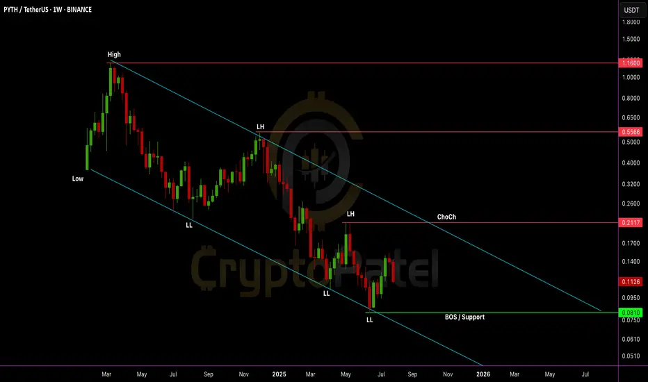
Will $PYTH go to $1 or drop even lower?Will EURONEXT:PYTH go to $1 or drop even lower?
Chart is still bearish with LL + LH structure.
But $0.0810 is a key level. If it holds, a trend reversal is possible. Accumulation zone: $0.085–$0.110
Risky entry, but R:R is huge. Hold = 10x potential to $1+
Break below $0.0810 = new LL incoming.
NFA & DYOR
is $VIRTUAL about to fly to $8?Don’t ignore this setup – is SPARKS:VIRTUAL about to fly to $8?
Price action is currently displaying a bullish flag structure on the daily chart — a continuation pattern following a strong impulse leg.
🔸 Impulse Move (Flagpole): +335% vertical rally
🔸 Consolidation Phase: Descending parallel channel forming the flag
🔸 Market Structure: Bullish continuation intact as long as the lower trendline holds
Technical Levels:
▪️ Support Zone: $1.30–$1.10 (confluence of demand & trendline support)
▪️ Breakout Confirmation: Clean daily close above $2.00 with elevated volume
▪️ Projected Target: $8.18 (measured move = flagpole height from breakout level)
Observations:
▪️ No structural breakdown observed — price respecting flag support
▪️ Volume remains muted during consolidation — typical in bullish flags
▪️ Breakout potential increases if price compresses toward apex with decreasing volatility
Invalidation: Break below $1.10 on high volume would shift bias neutral/bearish.
Strategy: Watch for breakout + retest confirmation above $2.00 to target $8.18. Risk can be defined below lower trendline support.
Note: NFa & DYOR

Institutional Intraday option Trading High Volume Trades: Institutions trade in huge lots, often influencing Open Interest.
Data-Driven Strategy: Backed by proprietary models, AI, and sentiment analysis.
Smart Order Flow: Institutions use algorithms to hide their positions using Iceberg Orders, Delta Neutral Strategies, and Volatility Skew.
⚙️ Tools & Indicators Used:
Option Chain Analysis
Open Interest (OI) & OI%
Put Call Ratio (PCR)
Implied Volatility (IV)
Max Pain Theory
Gamma Exposure (GEX)
🧠 Common Institutional Strategies:
Covered Calls – Generate income on large stock holdings.
Protective Puts – Hedge downside risk.
Iron Condor / Butterfly Spread – Capture premium with neutral view.
Long Straddle/Strangle – Expecting big move post-news.
Synthetic Longs/Shorts – Replicating stock exposure using options.

HeranbaSwing Trade -
Look interesting at current level - still closing pending
If today close above break out level
Maybe we can see Good move upside.
Risk around 8-10% around
Target next resistance

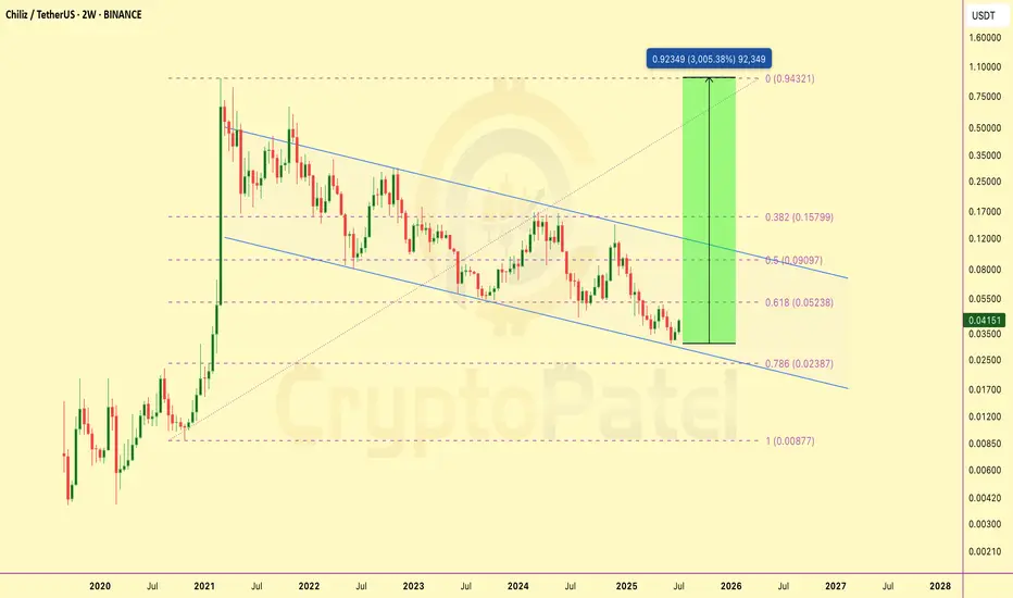
$CHZ did a 30x in 2021. Nobody cared until it was too lateBack in 2021, Chiliz ( GETTEX:CHZ ) delivered a 30x move — climbing from a $130M to $4B market cap in just a month. That move was fueled by strong fundamentals and massive hype around fan tokens.
Fast forward to now — price is sitting at the bottom of a multi-year falling wedge on the 2W timeframe. It just tapped the 0.786 Fibonacci retracement and showed a strong bounce with rising volume — a classic sign of potential reversal.
With solid partnerships, real-world utility, and a historical setup this clean, I’ve started building my position here. If the wedge breaks out, upside targets line up around $0.05 → $0.09 → $0.15 → $0.90 — back toward ATH levels.
Bottom might be in. Watch this closely.
Note: NFa & DYOR
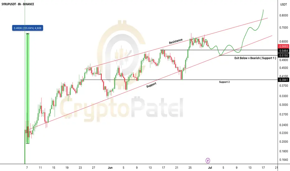
$SYRUP Price Prediction Analysis as per Ascending ChannelSYRUP/USDT – Technical Chart Update (8H Timeframe)
SYRUP is trading inside a clean ascending channel, showing a bullish structure with higher highs and higher lows.
Key Levels to Watch:
Support: $0.51
Resistance Targets: $0.70 → $0.80+
Exit Level: Bearish if price breaks below $0.51
Current Setup:
Price is respecting the lower trendline of the channel. A bounce here could lead to another leg up toward resistance.
Strategy:
Bullish bias as long as SYRUP holds above $0.51
Ideal zone to look for buy opportunities on dips
Exit or hedge if price closes below $0.51
Important Note:
If CRYPTOCAP:SYRUP holds the $0.51 support, it could soon enter the $1 club 🚀
But if it drops below $0.50, we may see a 30–50% retracement.
So always watch the chart closely before entering any trades.
Note: NFA & DYOR
Bitcoin Price Analysis 21-22 June 2025COINBASE:BTCUSD is in downtrend.
STRATEGY:
1. If the price breaks above the upper level, consider a long position. This is supported by the higher lows formation in a smaller timeframe, suggesting a continuation of the upward trend.
2. Bearish Scenario: If the price breaks below the lower level, consider a short position, targeting potential stop-loss orders or liquidity pools created during the higher lows formation.
AREA TO AVOID
Area between the upper and lower levels due to price consolidation.

NIFTY FINANCE H4, THERE'S POSSIBLITY OF SHORT THINGS FOUND
-T-LINE Breakdown & Retest
-Pending Liquidity
-Upside liquidity sweeped today
- HUGE GAP DOWN SIDE EXPECTED TO FILLED
TLL THEN , STAY FOCUSED
