How Geopolitical Events Influence Financial Markets1. Introduction to Geopolitics and Financial Markets
Financial markets—encompassing equities, bonds, commodities, foreign exchange, and derivatives—reflect the aggregate expectations of market participants regarding economic performance, corporate profitability, and global stability. Geopolitical events, by altering the perceived stability of economies, directly affect these expectations.
While domestic policies primarily influence local markets, geopolitical events often have transnational consequences. For example, a conflict in the Middle East can impact crude oil prices globally, which in turn affects inflation, interest rates, and stock markets worldwide. Similarly, U.S.-China trade tensions influence currency valuations, supply chains, and technology stocks globally.
2. Mechanisms of Geopolitical Influence
The impact of geopolitical events on financial markets occurs through several mechanisms:
a. Investor Sentiment and Risk Appetite
Markets are inherently psychological. Investors’ perceptions of risk and uncertainty drive buying or selling decisions. Geopolitical instability typically raises risk aversion, leading to capital flight from equities to safe-haven assets such as gold, U.S. Treasury bonds, and the Japanese yen.
Example: During the 2022 Russian invasion of Ukraine, global equities declined sharply as investors feared economic disruption. Simultaneously, gold prices surged, reflecting a flight to safety.
b. Commodity Price Volatility
Many geopolitical events directly impact commodities. Oil, natural gas, and rare earth metals are particularly sensitive. Disruptions in supply from geopolitically unstable regions can trigger sharp price swings.
Oil Markets: The Middle East, home to major oil exporters, often becomes a focal point. Tensions in the Persian Gulf or sanctions on oil-producing nations like Iran can spike crude prices, increasing inflationary pressures worldwide.
Agricultural Commodities: Conflicts in regions like Ukraine, a major grain exporter, can lead to global shortages and food price inflation, affecting stock markets and consumer confidence.
c. Currency and Foreign Exchange Markets
Geopolitical events influence capital flows and currency valuations. Investors often move capital toward perceived “safe” currencies during crises.
Safe-Haven Currencies: U.S. dollar, Swiss franc, and Japanese yen often strengthen during geopolitical uncertainty.
Emerging Market Vulnerability: Countries with high external debt in foreign currencies may face currency depreciation when global risk aversion rises.
d. Trade and Investment Flows
Trade wars, sanctions, and diplomatic tensions disrupt global supply chains and investment flows. Companies with international exposure can experience declining revenues and stock devaluation.
Example: U.S.-China trade tensions in 2018-2019 caused volatility in global equities, particularly in technology stocks reliant on cross-border supply chains.
e. Central Bank and Policy Reactions
Geopolitical events influence monetary and fiscal policies. Central banks may adjust interest rates or intervene in currency markets to mitigate economic shocks. Fiscal authorities may introduce stimulus or impose trade restrictions, influencing liquidity and market valuations.
Example: In response to the Ukraine crisis, European Central Bank (ECB) and other global banks closely monitored inflationary pressures from rising energy prices, influencing bond yields and stock market sentiment.
3. Historical Case Studies
a. Middle East Conflicts and Oil Prices
The oil crises of the 1970s illustrate how geopolitical shocks affect global markets. Political instability in the Middle East led to oil embargoes by OPEC nations, causing energy prices to quadruple. Stock markets plummeted, inflation surged, and recessionary pressures emerged worldwide.
Impact: Oil-dependent industries suffered losses; inflation-indexed bonds gained popularity as hedges; emerging markets faced balance-of-payment crises.
b. 9/11 Terrorist Attacks
The September 11, 2001 attacks in the U.S. created immediate panic in financial markets.
Equities: The New York Stock Exchange closed for several days; the Dow Jones Industrial Average fell over 14% in the following week.
Currencies: The U.S. dollar initially weakened but later strengthened as U.S. government spending increased.
Safe-Haven Assets: Gold and Treasury bonds saw increased demand.
c. Russia-Ukraine Conflict (2022-Present)
The ongoing conflict has had multifaceted effects:
Energy Prices: European natural gas prices surged, leading to energy market instability.
Agriculture: Ukraine’s role as a grain exporter caused disruptions in global food supply, raising prices.
Stock Markets: European equities experienced volatility due to geopolitical risk and economic sanctions.
Inflation: Energy-driven inflation forced central banks to revise monetary policies, impacting bond yields.
d. U.S.-China Trade War (2018-2019)
Tariffs and counter-tariffs created uncertainty in global trade and corporate earnings.
Stock Market Volatility: Technology and manufacturing sectors were most affected.
Supply Chains: Companies shifted manufacturing or sourcing to mitigate tariff impacts.
Emerging Markets: Countries integrated into global trade chains faced currency pressure and capital outflows.
4. Sectoral Impacts
Geopolitical events do not impact all sectors equally. Some sectors are more sensitive, while others may benefit:
Energy and Commodities: Oil, gas, and metals respond rapidly to geopolitical supply shocks.
Defense and Security: Military conflicts or heightened tensions often boost defense sector stocks.
Technology and Manufacturing: Global supply chains make these sectors vulnerable to trade restrictions and sanctions.
Consumer Goods: Inflationary pressures from geopolitical events reduce discretionary spending, affecting retail and luxury sectors.
5. Short-Term vs. Long-Term Impacts
a. Short-Term Volatility
Markets often react sharply to immediate news. High-frequency trading and algorithmic systems amplify reactions. Panic selling, liquidity crunches, and herd behavior dominate short-term responses.
Example: A missile strike or sudden announcement of sanctions can cause intraday or weekly spikes in volatility indices (e.g., VIX).
b. Long-Term Structural Changes
Some geopolitical events have enduring effects:
Supply Chain Restructuring: Companies may diversify sourcing to avoid future geopolitical risks.
Investment Patterns: Long-term capital allocation may shift to safer jurisdictions or sectors.
Energy Transition: Dependence on geopolitically unstable regions may accelerate renewable energy adoption.
6. Geopolitical Risk Measurement
Financial institutions use various tools to quantify and monitor geopolitical risk:
Geopolitical Risk Index (GPR): Measures newspaper coverage of geopolitical tensions.
Economic Policy Uncertainty Index: Tracks policy-related uncertainties affecting markets.
Volatility Indices: Market-implied volatility reflects risk perception, e.g., VIX for equities.
Credit Default Swaps (CDS): Reflect sovereign and corporate risk perception in conflict zones.
These metrics help investors hedge, diversify, and manage exposure.
7. Investor Strategies Amid Geopolitical Events
Investors employ several strategies to mitigate or capitalize on geopolitical risk:
a. Diversification
Spreading investments across countries, sectors, and asset classes reduces exposure to localized shocks.
b. Safe-Haven Assets
Gold, U.S. Treasuries, and stable currencies act as hedges during geopolitical turmoil.
c. Hedging with Derivatives
Options, futures, and swaps allow investors to hedge currency, commodity, or equity exposure during uncertain periods.
d. Tactical Allocation
Shifting allocations toward sectors likely to benefit from geopolitical developments (e.g., defense, energy) can enhance returns.
8. Challenges in Predicting Geopolitical Impact
Despite advanced analytics, predicting financial market reactions to geopolitical events remains challenging:
Complex Interdependencies: Global markets are interconnected; an event in one region can have cascading effects.
Behavioral Biases: Investor sentiment can overreact or underreact, creating volatility.
Policy Uncertainty: Government interventions can unpredictably amplify or mitigate market responses.
Time Horizon: Markets may react differently in the short term versus long term.
9. Emerging Trends
The modern financial landscape shows evolving dynamics of geopolitical influence:
Cybersecurity Threats: Geopolitical tensions increasingly manifest in cyberattacks, affecting technology and critical infrastructure.
Climate Diplomacy: Conflicts over resources like water or energy can influence commodity markets.
Globalization vs. Regionalization: Trade wars and sanctions push some nations toward regional supply chains, altering investment flows.
Technology and AI: Geopolitical competition in AI and semiconductors creates sector-specific investment risks.
10. Conclusion
Geopolitical events shape financial markets through a complex interplay of investor psychology, commodity prices, currency valuations, trade flows, and policy interventions. While short-term reactions often manifest as volatility and panic selling, long-term effects can restructure industries, supply chains, and investment strategies.
Investors, traders, and policymakers must remain vigilant, continuously monitoring global developments and adopting risk management strategies to navigate uncertainty. The ability to anticipate, analyze, and respond to geopolitical risk is now a fundamental skill in modern financial market participation.
In a globalized world, no market exists in isolation—geopolitical events in one corner of the planet can ripple across continents, affecting everything from energy prices to equities, bonds, and currencies. Understanding these linkages is not just advantageous—it is essential for sustainable and resilient financial decision-making.
Tradingidea
Breakout and Breakdown Trading1. Introduction to Breakout and Breakdown Trading
In financial markets, price movement is influenced by the forces of supply and demand. Traders identify key levels where these forces tend to converge and then anticipate movements when price “breaks out” above a resistance level or “breaks down” below a support level.
Breakout Trading: A strategy that involves entering a position when the price moves above a defined resistance level with the expectation of further upward momentum.
Breakdown Trading: The opposite approach, where traders enter a position when the price falls below a support level, anticipating a continuation of downward movement.
These strategies are rooted in technical analysis, relying on historical price action and market psychology rather than fundamental factors.
2. Core Concepts
2.1 Support and Resistance
Support: A price level where buying interest is strong enough to prevent further decline. It acts as a “floor.”
Resistance: A price level where selling pressure is strong enough to prevent further increase. It acts as a “ceiling.”
Breakouts occur when price surpasses resistance, while breakdowns happen when price falls below support.
2.2 Volume
Volume is a crucial confirmation tool. A breakout or breakdown is considered strong if accompanied by increased trading volume, as this indicates genuine market participation rather than a false move.
2.3 Price Consolidation
Before breakouts or breakdowns, prices often consolidate in tight ranges. These consolidations can be:
Rectangles
Triangles
Flags and pennants
Understanding the consolidation pattern helps traders anticipate the direction and magnitude of the breakout or breakdown.
3. Types of Breakouts and Breakdowns
3.1 Horizontal Breakouts
Occur when price breaks a clearly defined horizontal support or resistance.
Example: A stock repeatedly fails to move above $100. A breakout above $100 signals upward momentum.
3.2 Trendline Breakouts
Occur when price crosses a diagonal trendline drawn along highs or lows.
Uptrend breakout: Price breaks above a descending trendline.
Downtrend breakdown: Price falls below an ascending trendline.
3.3 Pattern-Based Breakouts
Certain chart patterns often precede strong breakouts or breakdowns:
Triangles: Symmetrical, ascending, or descending triangles
Rectangles: Price moves within a horizontal range
Flags and Pennants: Continuation patterns after a sharp move
Pattern-based breakouts tend to offer predictable price targets based on pattern dimensions.
4. Breakout Trading Strategy
4.1 Identifying a Breakout
Look for a well-defined resistance level or consolidation pattern.
Confirm breakout using volume: higher than average volume indicates strong buying interest.
Check for fundamental or news catalysts that may strengthen the breakout.
4.2 Entry Techniques
Aggressive Entry: Enter immediately when price crosses resistance.
Conservative Entry: Wait for a candle to close above resistance to confirm breakout.
4.3 Stop Loss Placement
Below the breakout point or recent swing low.
Helps protect against false breakouts.
4.4 Profit Targets
Use pattern-based targets: For triangles or rectangles, project the height of the pattern above breakout.
Use trailing stops to capture extended moves without exiting too early.
5. Breakdown Trading Strategy
5.1 Identifying a Breakdown
Look for a strong support level or consolidation pattern.
Check for rising selling volume: heavy selling confirms breakdown.
Identify any macroeconomic or sector-specific events that may accelerate declines.
5.2 Entry Techniques
Aggressive Entry: Enter immediately as the price breaks support.
Conservative Entry: Wait for a candle close below support to reduce risk.
5.3 Stop Loss Placement
Above the breakdown point or recent swing high.
Protects against false breakdowns where the price quickly recovers.
5.4 Profit Targets
Pattern-based projections: Use the height of the consolidation pattern subtracted from the breakdown point.
Trailing stops help lock in gains in volatile markets.
6. Psychological Aspects of Breakout and Breakdown Trading
Trading breakouts and breakdowns is as much psychological as technical:
6.1 Fear of Missing Out (FOMO)
Many traders enter too early due to FOMO, risking false breakouts.
Patience and confirmation reduce this risk.
6.2 Market Sentiment
Breakouts often occur when sentiment shifts from neutral or negative to bullish.
Breakdowns often coincide with panic selling or negative news.
6.3 Confirmation Bias
Traders may see a breakout or breakdown where none exists.
Strict adherence to predefined rules prevents bias-driven errors.
7. Common Mistakes and Risks
7.1 False Breakouts/Breakdowns
Occur when price briefly crosses support or resistance but reverses immediately.
Mitigation: Wait for candle close, confirm with volume, and consider broader market trend.
7.2 Overleveraging
Using excessive margin amplifies losses if breakout fails.
Always use proper risk management (1–2% of capital per trade).
7.3 Ignoring Market Context
Breakouts in choppy or low-liquidity markets are less reliable.
Always consider overall market trend, sector strength, and macroeconomic factors.
8. Tools and Indicators for Confirmation
8.1 Volume Indicators
On-Balance Volume (OBV)
Volume Oscillator
8.2 Momentum Indicators
RSI (Relative Strength Index): Confirms overbought or oversold conditions
MACD (Moving Average Convergence Divergence): Identifies trend shifts
8.3 Moving Averages
Help confirm breakout/breakdown trend direction.
Common strategy: Wait for price to cross above/below 20-day or 50-day moving average.
9. Examples of Breakout and Breakdown Trading
9.1 Breakout Example
Stock consolidates between $50–$55.
Breaks above $55 on heavy volume, closing at $56.
Entry: $56
Stop Loss: $54.50 (below consolidation)
Target: $61 (height of consolidation added to breakout level)
9.2 Breakdown Example
Stock trades between $70–$65.
Falls below $65 with high volume, closing at $64.
Entry: $64
Stop Loss: $66 (above consolidation)
Target: $59 (height of consolidation subtracted from breakdown level)
10. Advanced Techniques
10.1 Pullback Entry
After breakout, price often retests the breakout level.
Provides lower-risk entry opportunities.
10.2 Multiple Timeframe Analysis
Confirm breakout on higher timeframe (daily or weekly) while entering on lower timeframe (hourly or 15-min).
Reduces the likelihood of false breakouts.
10.3 Combining with Fundamental Analysis
Breakouts accompanied by strong earnings, positive news, or macroeconomic support have higher reliability.
Breakdowns following negative news or sector weakness confirm downward trend.
Conclusion
Breakout and breakdown trading is a cornerstone of technical trading, blending market psychology, price action, and disciplined risk management. While the concept is simple—buy above resistance and sell below support—the execution requires attention to volume, patterns, market context, and trading psychology. Traders who master these strategies can capitalize on strong momentum moves and manage risk effectively.
Successful breakout and breakdown trading hinges on patience, confirmation, proper entry and exit points, and disciplined risk management. By combining technical indicators, volume analysis, and pattern recognition, traders can improve the probability of capturing meaningful market moves while avoiding the pitfalls of false signals.
Zero-Day Option TradingIntroduction
Zero-Day Option Trading (ZDOT), also referred to as 0DTE (Zero Days to Expiration) trading, has gained significant traction in the last few years, particularly among professional traders and high-frequency retail traders. The strategy revolves around trading options contracts that expire on the same day, often within hours. This ultra-short-term trading method leverages rapid price movements, time decay, and market volatility to generate potential profits.
While zero-day options present extraordinary opportunities, they also carry significant risk due to their extreme sensitivity to market movements and time decay. Understanding ZDOT requires knowledge of option pricing, market mechanics, strategies, and risk management.
Understanding Options Basics
Before diving into zero-day options, it is essential to revisit the fundamentals of options trading.
Options Types
Call Options: Give the holder the right, but not the obligation, to buy an underlying asset at a predetermined price (strike price) before expiration.
Put Options: Give the holder the right, but not the obligation, to sell an underlying asset at a predetermined price before expiration.
Option Pricing Factors
Options prices are derived from models like the Black-Scholes Model and are influenced by:
Underlying Asset Price: Directly affects the intrinsic value.
Strike Price: Determines whether the option is in-the-money (ITM), at-the-money (ATM), or out-of-the-money (OTM).
Time to Expiration (Theta): Represents time decay; the closer to expiry, the faster an option loses value.
Volatility (Vega): Higher volatility increases the option premium.
Interest Rates and Dividends: Affect the option's theoretical price marginally.
Option Greeks
Understanding Greeks is crucial in ZDOT because the risk-reward profile changes rapidly:
Delta (Δ): Measures the option’s price sensitivity to the underlying asset price.
Gamma (Γ): Measures the rate of change of delta; higher gamma means price reacts sharply to underlying moves.
Theta (Θ): Measures time decay; for zero-day options, theta is extremely high.
Vega (ν): Measures sensitivity to volatility.
Rho (ρ): Measures sensitivity to interest rates (less relevant for ZDOT).
What Are Zero-Day Options?
Zero-day options are options contracts that expire the same day they are traded. For example, if an S&P 500 index option expires on a Friday, a trader could enter a trade on Friday morning, and the contract would expire by market close.
Key characteristics include:
Ultra-Short Expiry: Time decay is at its peak, and option value is primarily extrinsic premium.
High Gamma: Small moves in the underlying asset lead to large changes in option delta.
Rapid Time Decay: Theta accelerates as the expiration hour approaches, making options highly sensitive.
High Liquidity (for popular underlyings): Index options (like SPX, NIFTY, or ES futures options) often offer tight spreads and high volume.
Speculative Nature: Traders often use these options for intraday speculation rather than long-term investment.
Why Zero-Day Options Have Gained Popularity
Several factors contribute to the rise of zero-day option trading:
Low Capital Requirement: Traders can take positions on small premium options with relatively low capital.
Leverage: Due to low cost and high delta, traders can control large exposure to the underlying asset.
High Reward Potential: Rapid price swings in the underlying asset can generate significant profits.
Advanced Technology and Platforms: High-frequency trading, algorithmic strategies, and low-latency platforms make execution faster.
Volatility-Based Strategies: Intraday volatility spikes (like FOMC announcements, economic data releases, or corporate earnings) create opportunities for short-term traders.
How Zero-Day Options Work
1. Time Decay (Theta)
Zero-day options are almost entirely driven by time decay. Theta measures the rate at which the option loses extrinsic value:
For long option holders, the value decays extremely fast.
For short option sellers, theta works in their favor as options lose value rapidly as expiration approaches.
Example:
A call option on NIFTY at-the-money might lose 50–70% of its value in the last few hours of trading due to accelerated theta.
2. Delta and Gamma
Delta indicates the likelihood of the option ending in-the-money:
At-the-money (ATM) zero-day options have a delta near 0.5.
Gamma is extremely high for ATM zero-day options, meaning small movements in the underlying asset can swing the delta dramatically.
Traders can quickly move from profitable to loss positions or vice versa.
3. Volatility (Vega)
Vega sensitivity diminishes as expiration nears.
ZDOT primarily focuses on underlying price movement rather than changes in implied volatility.
Volatility spikes can still create profitable opportunities, especially during market open or news events.
4. Liquidity and Execution
SPX, NIFTY, ES, and other major indices offer high liquidity.
Tight bid-ask spreads reduce slippage and execution risk.
Deep liquidity is essential as zero-day trading relies on quick entry and exit.
Common Zero-Day Option Strategies
Traders employ several strategies depending on their risk tolerance and market outlook. These can broadly be divided into directional and non-directional strategies.
1. Directional Strategies
These strategies assume a specific price movement in the underlying asset:
a. Buying ATM Calls or Puts
Traders speculate on intraday price movement.
High gamma can turn small moves into significant profits.
High risk due to rapid theta decay.
b. Long Straddle
Buying ATM call and put simultaneously.
Profitable if underlying moves sharply in either direction.
Risk: If the market remains flat, both options decay quickly.
c. Long Strangle
Buying slightly OTM call and put.
Less expensive than straddle.
Requires a larger move to become profitable.
2. Non-Directional / Theta-Based Strategies
These strategies aim to profit from time decay rather than directional moves:
a. Short Straddle
Selling ATM call and put simultaneously.
Profits if the market remains stable.
Extremely risky if underlying moves sharply.
b. Short Strangle
Selling OTM call and put.
Less risky than straddle, but still vulnerable to large moves.
c. Iron Condor
Selling OTM call and put while buying further OTM options for risk protection.
Profitable in low-volatility markets.
Limited risk, limited reward.
Risk Management in Zero-Day Option Trading
Zero-day trading is inherently high-risk. Effective risk management is critical for survival:
Position Sizing
Avoid allocating more than 1–2% of capital per trade.
Use small, calculated trades to minimize the risk of a total loss.
Stop Losses
Intraday exit rules are essential.
Some traders use delta-neutral stop-loss triggers or predefined percentage losses.
Hedging
Short and long combinations like iron condors provide built-in hedges.
Delta-hedging strategies can neutralize directional risk.
Volatility Awareness
Avoid trading near extreme market events unless prepared for rapid moves.
Sudden volatility spikes can wipe out short positions in seconds.
Market Hours and Liquidity
Trade during the most liquid periods (e.g., market open and last hour).
Avoid trading in illiquid or thinly traded instruments.
Advantages of Zero-Day Option Trading
High Profit Potential
The leverage effect of options can lead to significant intraday gains.
Rapid Feedback
Traders quickly see results, allowing rapid learning and strategy adjustments.
Flexibility
Both directional and non-directional strategies can be employed.
Scalability
Strategies can be applied across indices, stocks, commodities, and ETFs.
Disadvantages and Risks
Extreme Risk
A single wrong move can result in 100% loss of the premium for long options or unlimited loss for naked shorts.
Requires Expertise
Understanding Greeks, market microstructure, and timing is crucial.
Psychological Pressure
High-speed trading can induce stress and emotional errors.
Limited Margin for Error
Zero-day options leave no room for delayed reaction or misjudgment.
Practical Tips for Traders
Start Small
Begin with minimal exposure to learn the mechanics.
Focus on Highly Liquid Instruments
SPX, NIFTY, and ES are preferred due to tight spreads.
Use Technical Analysis
Short-term support, resistance, and intraday momentum patterns can guide entry and exit.
Combine Strategies
Blend directional bets with non-directional strategies to manage risk.
Track News Events
Economic releases and earnings can cause rapid price swings suitable for zero-day trades.
Regulatory and Brokerage Considerations
Some brokers restrict zero-day option trading due to high risk.
Margin requirements may be higher for selling options.
Traders must be aware of regulatory guidelines in their region (e.g., SEBI in India, SEC in the U.S.).
Conclusion
Zero-Day Option Trading is a high-risk, high-reward intraday trading technique that has gained popularity due to low capital requirements, rapid time decay, and leverage opportunities. While it offers extraordinary profit potential, the strategy demands discipline, expertise, and rigorous risk management. Traders must understand option Greeks, market volatility, liquidity, and intraday technical patterns to succeed.
For beginners, zero-day trading should be approached cautiously, starting with small trades and focusing on education. For experienced traders, it offers a tool to exploit rapid market movements, hedge positions, or implement advanced strategies like gamma scalping.
In essence, ZDOT is not for the faint-hearted—it is a strategy where precision, timing, and strategy execution determine success. With proper planning and discipline, zero-day option trading can be a powerful component of an intraday trader’s toolkit.

Part 1 Intraday Master ClassIntroduction to Option Trading
Option trading is one of the most dynamic, flexible, and powerful financial instruments in the modern market. It allows investors not only to profit from price movements but also to protect their portfolios, speculate, or earn regular income. Unlike buying stocks directly, options give traders the right but not the obligation to buy or sell an underlying asset (like a stock, index, or commodity) at a predetermined price within a certain time frame.

MARUTI 1 Month Time Frame 📊 Monthly Support & Resistance Levels
Based on pivot point analysis, here are the key levels to watch:
Pivot Point (PP): ₹16,163.67
Resistance Levels: ₹16,416.33 (R1), ₹16,567.67 (R2), ₹16,820.33 (R3)
Support Levels: ₹16,012.33 (S1), ₹15,759.67 (S2), ₹15,608.33 (S3)
These levels are derived from standard pivot point calculations and can serve as potential entry or exit points for traders.
Technical Indicators
Relative Strength Index (RSI): Currently at 59.15, indicating that the stock is not yet overbought and may have room for further upside.
Moving Averages: The stock is trading above its 50-day and 200-day moving averages, confirming an uptrend.
MACD: The Moving Average Convergence Divergence (MACD) is positive, suggesting bullish momentum.
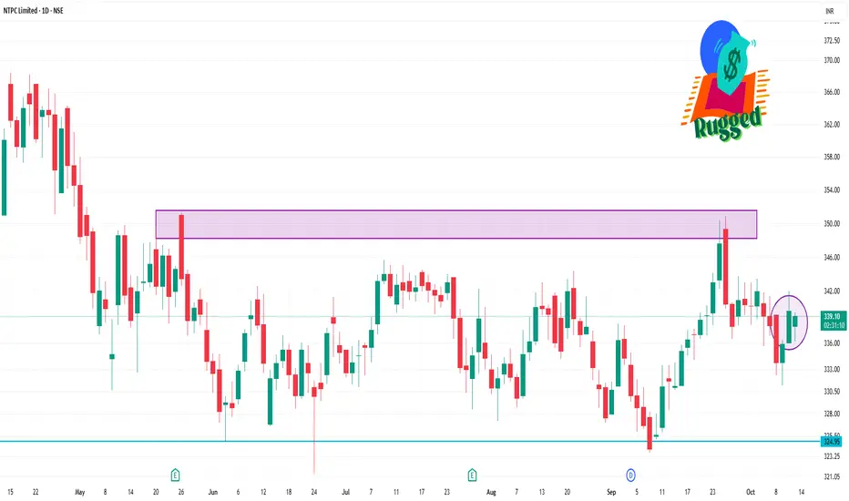
NTPC 1 Day Time Frame📈 Intraday Support & Resistance Levels
Immediate Support: ₹337.29
Immediate Resistance: ₹340.85
Key Pivot Point: ₹339.20
These levels are derived from standard pivot point calculations and are commonly used by traders for short-term strategies.
🔍 Technical Indicators
Relative Strength Index (RSI): 53.93 — indicating a neutral market condition.
Moving Average Convergence Divergence (MACD): 0.330 — suggesting a bullish trend.
5-Day Moving Average: ₹338.45 — supporting a bullish outlook.
50-Day Moving Average: ₹338.05 — reinforcing the bullish trend.
200-Day Moving Average: ₹336.12 — indicating long-term bullish sentiment.
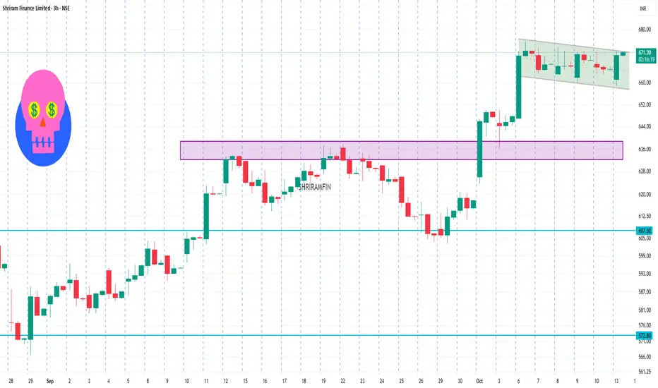
SHRIRAMFIN 3 Hour Time Frame📊 3-Hour Timeframe Technical Levels
Current Price: ₹669.70
Pivot Points:
S1: ₹666.48
Pivot: ₹669.97
R1: ₹674.88
R2: ₹678.37
R3: ₹682.87
Fibonacci Levels:
Retracement:
23.6%: ₹658.34
38.2%: ₹647.73
50%: ₹639.15
61.8%: ₹630.57
76.4%: ₹619.96
Projection:
23.6%: ₹682.21
38.2%: ₹692.82
50%: ₹701.40
61.8%: ₹709.98
76.4%: ₹720.59
Extension:
123.6%: ₹753.14
138.2%: ₹775.18
150%: ₹793.00
161.8%: ₹810.82
176.4%: ₹832.86
Camarilla Levels:
R4: ₹669.67
R3: ₹666.59
R2: ₹663.51
R1: ₹660.43
S1: ₹657.72
S2: ₹654.07
S3: ₹650.55
S4: ₹647.83
Woodie's Levels:
R1: ₹669.25
R2: ₹674.53
R3: ₹679.25
S1: ₹660.85
S2: ₹657.72
S3: ₹654.57
Demark Levels:
R1: ₹668.23
R2: ₹672.50
S1: ₹659.82
S2: ₹665.30
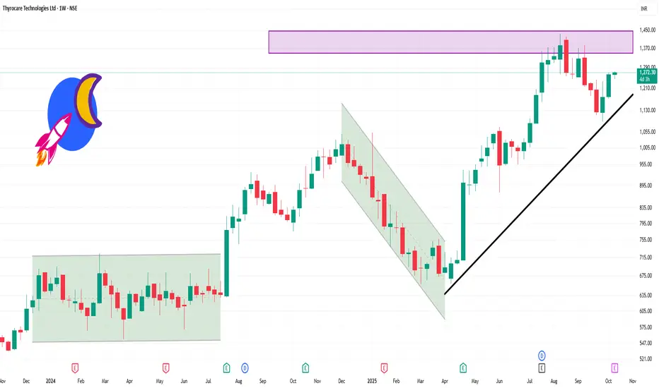
THYROCARE 1 Week Time Frame 📈 1-Week Performance Snapshot
Current Price (Oct 10, 2025): ₹1,264.00
Weekly Gain: Approximately +4.76%
Weekly Range: ₹1,205.80 – ₹1,270.50
This upward trend is supported by increased trading volume, indicating strong investor interest.
🔍 Technical Indicators
Support Levels: ₹1,246.35 and ₹1,208.21
Resistance Levels: ₹1,337.05
Moving Averages: Short-term indicators suggest a bullish outlook, though a potential correction could occur if support levels are breached
📊 Additional Insights
Market Capitalization: ₹6,664.05 crore
P/E Ratio: 62.52
Dividend Yield: 1.66%
52-Week High/Low: ₹1,435.00 / ₹658.00
These metrics position Thyrocare as a significant player in the healthcare sector, with robust financials and a consistent dividend history.
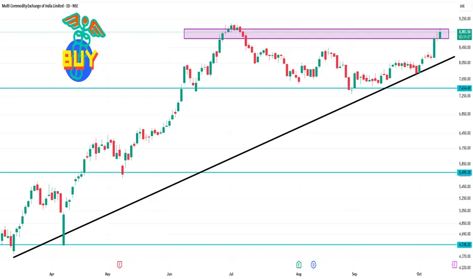
MCX 1 Day Time Frame Opening Price: ₹8,700.00
Day’s High: ₹8,988.00
Day’s Low: ₹8,700.00
Previous Close: ₹8,688.50
Volume: 610,010 shares traded
VWAP (Volume-Weighted Average Price): ₹8,893.80
Technical Indicators:
According to TradingView, the 1-day technical analysis for MCX indicates a strong buy signal, with the majority of indicators, including moving averages and oscillators, supporting this trend. However, the oscillator readings are currently neutral, suggesting a balanced market momentum.
Divergence SecretsThere are two main types of options: Call Options and Put Options.
A Call Option gives the buyer the right to buy an asset at a predetermined price, called the strike price, before the expiry date. Investors buy calls when they expect the price of the underlying asset to rise.
A Put Option, on the other hand, gives the buyer the right to sell an asset at the strike price before expiry. Traders buy puts when they expect the asset’s price to fall.

Part 1 Support and Resistance Option Pricing – The Greeks
Option pricing is influenced by several factors such as the underlying price, time to expiry, volatility, and interest rates. These factors are represented by “Greeks,” which measure the sensitivity of an option’s price to different variables:
Delta (Δ): Measures how much the option price changes with a ₹1 move in the underlying asset.
Gamma (Γ): Measures the rate of change of Delta — i.e., how stable Delta is.
Theta (Θ): Measures time decay — how much value the option loses each day as expiry nears.
Vega (ν): Measures sensitivity to volatility — how much the option price changes with changes in market volatility.
Rho (ρ): Measures sensitivity to interest rates.
Understanding these helps traders build strategies that match their risk tolerance and market view.

Option Trading Participants in Option Trading
There are generally four types of participants in the options market:
Buyers of Calls: Expect the price of the underlying to go up.
Sellers (Writers) of Calls: Expect the price to remain the same or fall.
Buyers of Puts: Expect the price of the underlying to go down.
Sellers (Writers) of Puts: Expect the price to remain the same or rise.
Buyers have limited risk (the premium paid) and unlimited profit potential, while sellers have limited profit (premium received) but unlimited potential risk.

Part 1 Candle Stick PatternKey Terminology in Options
Before diving deeper, understanding these basic terms is essential:
Strike Price: The price at which the option can be exercised.
Premium: The price paid by the buyer to purchase the option.
Expiry Date: The date on which the option contract ends.
In the Money (ITM): When exercising the option gives a profit (e.g., a call option when the stock price is above the strike price).
Out of the Money (OTM): When exercising the option gives a loss (e.g., a call option when the stock price is below the strike price).
At the Money (ATM): When the stock price and strike price are almost the same.
Underlying Asset: The financial instrument (like a stock, index, or currency) on which the option is based.

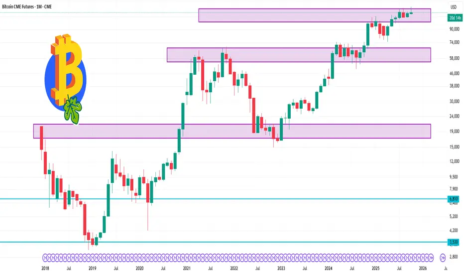
Bitcoin 1 Month Time frame 📊 1-Month Price Range
High: $123,270
Low: $113,150
Current: $116,990
52-Week Range: $59,990 – $127,240
🔍 Technical Overview
The 1-month technical analysis for BTC.1 indicates a neutral market sentiment, with no strong buy or sell signals.
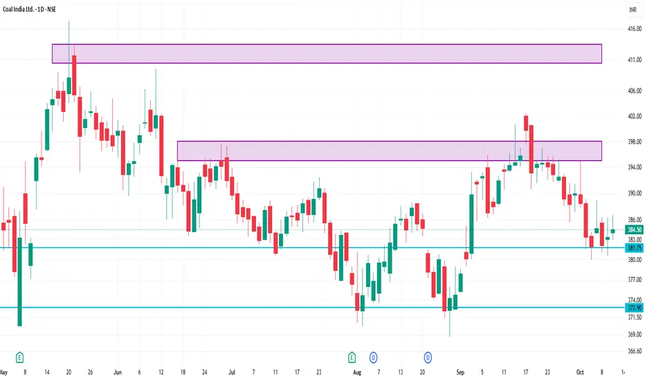
COALINDIA 1 Day Time Frame 📊 Key Intraday Levels
Support Levels: ₹382.95 – ₹383.35
Resistance Levels: ₹386.70 – ₹387.85
Day Range: ₹382.95 – ₹386.70
Previous Close: ₹383.35
Upper Circuit Limit: ₹421.65
Lower Circuit Limit: ₹345.05
52-Week Range: ₹349.25 – ₹502.45
🔍 Technical Indicators
Pivot Points: Central Pivot at ₹389.17, with resistance at ₹391.20 and support at ₹388.55.
Candlestick Patterns: Recent sessions have shown patterns like Harami Bullish and Doji, indicating indecision and possible reversal attempts.
Relative Strength Index (RSI): The 14-day RSI is at 48.52, suggesting a neutral market condition.
📈 Summary
Coal India Ltd is currently trading near its support level of ₹383.35. A breakout above ₹387.85 could signal a bullish trend, while a decline below ₹382.95 may indicate a bearish move. Technical indicators suggest a neutral market condition, with recent candlestick patterns indicating indecision and possible reversal attempts.
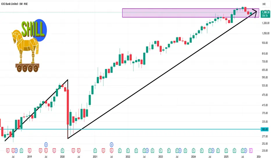
ICICIBANK 1 Month Time Frame 📊 Monthly Technical Levels
Pivot Point: ₹1,374.47
Support Levels:
S1: ₹1,316.13
S2: ₹1,284.27
S3: ₹1,225.93
Resistance Levels:
R1: ₹1,406.33
R2: ₹1,464.67
R3: ₹1,496.53
These levels are derived from standard pivot point calculations and can serve as key reference points for traders.
🔍 Technical Indicators
Relative Strength Index (RSI): Currently at 46.06, indicating a neutral condition, suggesting no immediate overbought or oversold conditions.
Moving Averages: The stock is showing a buy signal across various moving averages, with 8 buy signals and 4 sell signals, suggesting a bullish trend.
Technical Indicators: A strong buy signal is observed, with 10 buy signals and no sell signals, indicating positive momentum.
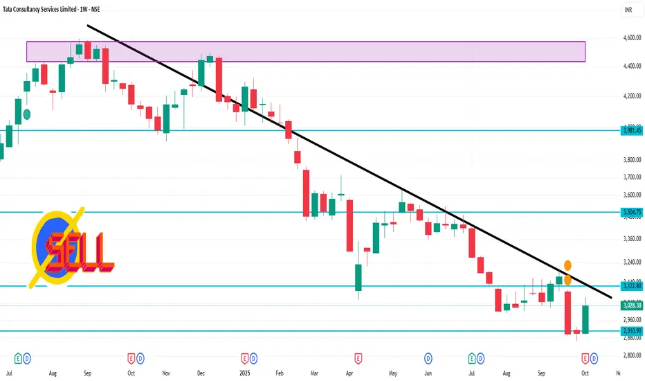
TCS 1 Week Time Frame Weekly Technical Overview
Current Price: ₹3,028.30 on the NSE
52-Week Range: ₹2,866.60 – ₹4,494.90
Volume: Approximately 8.8 million shares traded this week
VWAP: ₹3,032.15
Market Cap: ₹1.095 trillion
Beta: 0.97 (indicating moderate volatility
🔍 Key Technical Indicators
Moving Averages: TCS is trading below its 200-day moving average, suggesting a bearish trend.
RSI: The Relative Strength Index is in the neutral zone, indicating balanced buying and selling pressures.
MACD: The Moving Average Convergence Divergence is showing a bearish crossover, which may signal a potential downward movement.
📈 Outlook
Support Levels: Immediate support is observed around ₹2,950, with a stronger support zone near ₹2,870.
Resistance Levels: Key resistance is at ₹3,100, followed by ₹3,200.
Volatility: The stock's beta of 0.97 suggests that it moves in line with the broader market, with moderate volatility.
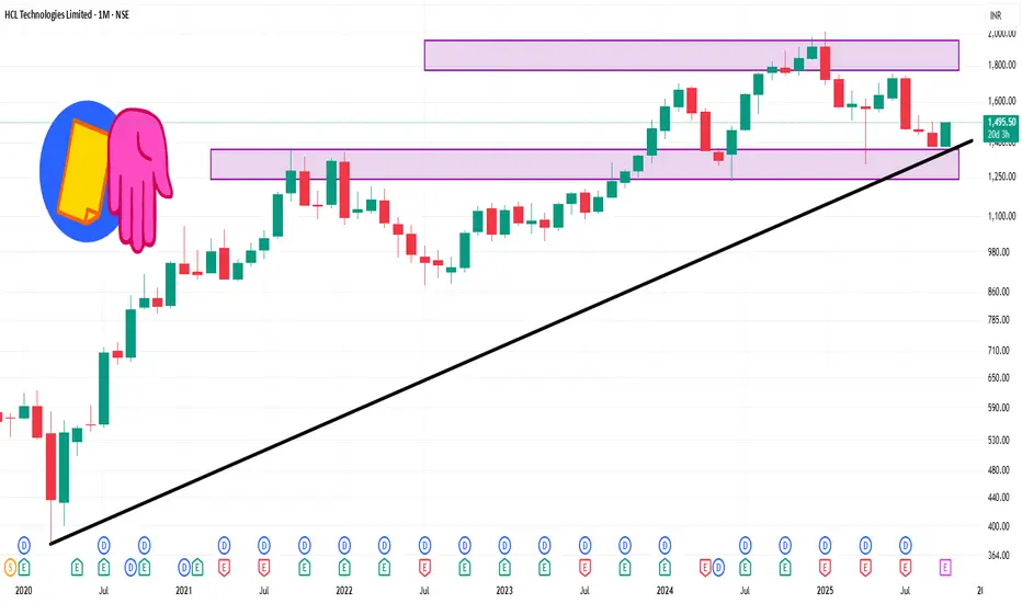
HCLTECH 1 Month Time Frame 📈 1-Month Performance Overview
Current Price: ₹1,495.50
1-Month Change: +4.19%
52-Week Range: ₹1,302.75 – ₹2,012.20
Market Capitalization: ₹4,05,612 crore
P/E Ratio (TTM): 23.88
Dividend Yield: 4.02%
Over the past month, HCL Technologies has shown a steady upward trend, outperforming the Nifty IT Index, which has gained approximately 0.33% during the same period.
📊 Technical Snapshot
1-Month High: ₹1,502.90
1-Month Low: ₹1,380.40
Average Price: ₹1,443.09
Price Change: +2.16%
Algorithmic Trading in India1. Introduction to Algorithmic Trading
Algorithmic trading refers to the use of computer algorithms to automate the process of trading financial securities — such as stocks, derivatives, commodities, or currencies — based on predefined rules and market conditions. These algorithms analyze market data, identify trading opportunities, and execute buy or sell orders with minimal human intervention.
At its core, algorithmic trading combines finance, mathematics, and computer science to create intelligent trading systems that can process information and act faster than any human trader. These systems follow strict quantitative models to determine the timing, price, and volume of trades to achieve optimal results.
In India, algorithmic trading gained popularity after the National Stock Exchange (NSE) introduced Direct Market Access (DMA) in 2008, allowing institutional investors to place orders directly into the market using automated systems. Over time, the technology has become more sophisticated, enabling both institutional and retail participation.
2. Evolution of Algorithmic Trading in India
The evolution of algo trading in India can be divided into distinct phases:
a. Pre-2000: Manual Trading Era
Before 2000, most trades were executed manually on the exchange floor. Brokers used phone calls and physical slips to place orders. This process was time-consuming, error-prone, and inefficient.
b. 2000–2010: Electronic Trading Emerges
With the digital transformation of the NSE and BSE, electronic order matching systems replaced the open outcry method. By 2008, the introduction of DMA and co-location facilities laid the foundation for algorithmic and high-frequency trading (HFT).
c. 2010–2020: Rise of Quantitative Strategies
Institutional investors and hedge funds started employing quantitative trading models to gain an edge in execution and strategy. The Securities and Exchange Board of India (SEBI) also began formulating guidelines to regulate algorithmic trading practices, ensuring fairness and transparency.
d. 2020–Present: Democratization and Retail Adoption
With advancements in technology, lower computing costs, and the rise of retail trading platforms (like Zerodha, Upstox, and Dhan), algorithmic trading tools have become accessible to individual investors. Today, APIs, Python-based strategies, and machine learning models are widely used by Indian traders to automate their trades.
3. How Algorithmic Trading Works
Algorithmic trading operates through a systematic process involving data analysis, model development, order execution, and monitoring. Here’s a simplified overview:
Market Data Collection:
Algorithms collect large volumes of market data in real time, including price, volume, and volatility metrics.
Signal Generation:
Based on mathematical models and indicators, the algorithm identifies trading opportunities. For example, if a moving average crossover occurs, it may trigger a buy signal.
Order Execution:
Once a signal is generated, the algorithm places orders automatically through an API or exchange gateway.
Risk Management:
Algorithms include predefined risk controls like stop losses, position sizing, and exposure limits to prevent large losses.
Backtesting and Optimization:
Before deployment, strategies are tested on historical data to validate performance under various market conditions.
Live Monitoring:
After implementation, algorithms are continuously monitored for slippage, latency, and performance.
4. Regulatory Framework in India
The Securities and Exchange Board of India (SEBI) regulates algorithmic trading to maintain market integrity and prevent unfair practices. Some key regulations include:
Exchange Approval:
Brokers and firms must obtain exchange approval for deploying algorithmic strategies.
Order-to-Trade Ratio:
To prevent market overload, SEBI has imposed limits on the ratio of orders to actual trades.
Risk Controls:
Mandatory controls such as price band checks, quantity limits, and self-trade prevention are required.
Co-location and Latency Equalization:
Exchanges provide co-location facilities (servers near exchange data centers) to minimize latency, though SEBI monitors for potential unfair advantages.
Audit Trail:
All algorithmic trades must have complete audit trails for transparency and accountability.
Retail Algorithmic Trading Guidelines (2022):
SEBI recently proposed a framework for retail algo trading via APIs, ensuring that brokers vet and approve algorithms before deployment.
This regulatory vigilance has allowed India to balance innovation with investor protection.
5. Benefits of Algorithmic Trading
Algorithmic trading has numerous advantages over manual methods:
a. Speed and Efficiency
Algorithms can analyze and execute thousands of trades in milliseconds, far faster than any human could.
b. Elimination of Emotion
By following pre-coded rules, algo systems eliminate emotional biases such as fear and greed, leading to disciplined trading.
c. Lower Transaction Costs
Automation reduces manual intervention, improving execution quality and minimizing brokerage costs.
d. Improved Liquidity
With higher trading volumes and tighter spreads, liquidity in the markets improves, benefiting all participants.
e. Enhanced Risk Management
Predefined risk parameters ensure controlled exposure and prevent large drawdowns.
f. Consistent Strategy Execution
Algorithms ensure consistent and accurate execution of strategies without deviation due to human fatigue or emotion.
6. Popular Algorithmic Trading Strategies in India
Several quantitative strategies are commonly deployed by Indian traders and institutions:
a. Trend-Following Strategies
These rely on indicators like Moving Averages, MACD, and RSI to identify momentum and follow the direction of the market trend.
b. Mean Reversion Strategies
These assume that prices will revert to their mean over time. Bollinger Bands and RSI divergence are typical indicators used.
c. Arbitrage Strategies
Exploiting price differences across exchanges or instruments, such as cash-futures arbitrage or inter-exchange arbitrage, to generate risk-free profits.
d. Statistical Arbitrage
Uses complex mathematical models to identify mispriced securities in correlated pairs or baskets.
e. Market Making
Involves placing simultaneous buy and sell orders to profit from the bid-ask spread while providing liquidity.
f. News-Based or Event-Driven Trading
Algorithms use NLP (Natural Language Processing) to interpret news or social sentiment and execute trades based on real-time events.
g. High-Frequency Trading (HFT)
Involves ultra-fast order execution and minimal holding times to exploit micro price movements, typically used by institutions.
7. Technologies Behind Algorithmic Trading
Algorithmic trading relies on an integration of cutting-edge technologies:
Programming Languages:
Python, C++, Java, and R are widely used for coding strategies and handling data.
APIs and Market Data Feeds:
APIs like Zerodha Kite Connect, Upstox API, and Interactive Brokers API allow real-time market access.
Machine Learning & AI:
Predictive models using neural networks, regression, and reinforcement learning enhance decision-making accuracy.
Cloud Computing:
Cloud-based deployment enables low-latency processing and scalability.
Big Data Analytics:
Helps in analyzing terabytes of market and sentiment data for pattern recognition.
Blockchain Integration (Emerging):
Enhances transparency and security in trade settlements.
8. Challenges and Risks in Algorithmic Trading
Despite its advantages, algorithmic trading comes with its share of risks:
a. Technical Failures
System glitches or connectivity issues can lead to massive losses in seconds.
b. Overfitting
Strategies that perform well on historical data may fail in real markets due to over-optimization.
c. Latency Issues
Even microseconds of delay can make or break an HFT strategy.
d. Market Manipulation Risks
Flash crashes or spoofing (placing fake orders) can disrupt markets.
e. High Costs for Infrastructure
Co-location servers and data feeds can be expensive for smaller firms.
f. Regulatory Complexity
Constantly evolving SEBI regulations require compliance and technical audits, adding to operational overhead.
9. Retail Participation and the Rise of DIY Algo Trading
One of the most exciting developments in India’s market landscape is the growing retail participation in algorithmic trading.
Platforms like Streak, AlgoTest, Tradetron, and Dhan Algo Lab have simplified algo development for individual traders by providing drag-and-drop interfaces, backtesting tools, and prebuilt strategies.
Retail traders can now:
Build and deploy algos without coding.
Use Python notebooks to design custom strategies.
Access historical market data for analysis.
Automate trades through broker APIs.
This democratization of technology is reshaping the retail trading landscape, allowing individuals to compete in efficiency with institutional players.
10. The Future of Algorithmic Trading in India
The future of algorithmic trading in India looks highly promising. Several trends are shaping its trajectory:
a. Artificial Intelligence Integration
AI-powered systems will increasingly predict market behavior, making trading smarter and adaptive.
b. Quantum Computing
The potential for near-instantaneous computation could revolutionize complex trading models.
c. Blockchain-Based Settlements
Blockchain could bring greater efficiency and transparency to clearing and settlement processes.
d. Wider Retail Access
As costs decrease and regulations evolve, retail traders will gain greater access to institutional-grade tools.
e. Cross-Market Integration
Algo systems will expand to commodities, currency markets, and international exchanges, creating a unified global trading environment.
f. Regulatory Innovation
SEBI’s proactive approach ensures that the market remains transparent and competitive, promoting sustainable growth.
11. Conclusion
Algorithmic trading represents the future of financial markets in India. What began as a niche practice among institutional investors has now become a mainstream phenomenon, empowering traders with data-driven precision and unmatched efficiency.
With strong regulatory oversight, robust technological infrastructure, and increasing retail adoption, India’s algorithmic trading ecosystem is poised for exponential growth. However, traders must approach automation with responsibility — focusing on robust strategy design, risk management, and compliance.
In essence, algorithmic trading in India symbolizes a perfect blend of technology and finance, paving the way for smarter, faster, and more efficient markets — where innovation meets opportunity.
Master Technical Indicators1. Understanding Technical Indicators
A technical indicator is a mathematical calculation based on price, volume, or open interest of a security or asset. Indicators are plotted on charts to help traders visualize trends, reversals, and potential entry or exit points.
Traders use these indicators to simplify the complexity of raw price data. Rather than analyzing each candle or tick, indicators smooth out noise and highlight the underlying strength or weakness of a trend. They are particularly effective when used alongside chart patterns, price action, and market sentiment analysis.
Why Are Technical Indicators Important?
They help identify the direction of a trend (up, down, or sideways).
They signal potential entry and exit points.
They assist in determining market strength and volatility.
They provide confirmation for trade setups.
They help in risk management by defining stop-loss and target zones.
2. Types of Technical Indicators
Technical indicators are generally classified into four main categories:
a. Trend Indicators
These show the direction and strength of a market trend.
Examples: Moving Averages, MACD, Average Directional Index (ADX), Parabolic SAR.
b. Momentum Indicators
These measure the speed of price movements, helping traders spot overbought or oversold conditions.
Examples: RSI, Stochastic Oscillator, CCI, Momentum Indicator.
c. Volatility Indicators
They measure the rate of price change or fluctuations, showing how much an asset moves over a specific time period.
Examples: Bollinger Bands, ATR (Average True Range), Donchian Channels.
d. Volume Indicators
Volume-based indicators analyze the strength behind price movements, helping traders confirm trends or reversals.
Examples: On-Balance Volume (OBV), Volume Oscillator, Chaikin Money Flow (CMF).
3. Top Technical Indicators Every Trader Should Master
Let’s dive deep into the most powerful and widely used technical indicators.
a. Moving Averages (MA)
The Moving Average is one of the simplest yet most powerful tools in technical analysis. It smooths price data to identify the direction of the trend.
Types:
Simple Moving Average (SMA) – Calculates the average price over a specific period.
Exponential Moving Average (EMA) – Gives more weight to recent prices, making it more responsive.
How Traders Use It:
Trend Identification:
When price is above the moving average, it indicates an uptrend; below it indicates a downtrend.
Crossovers:
Golden Cross: When the short-term MA crosses above the long-term MA (bullish signal).
Death Cross: When the short-term MA crosses below the long-term MA (bearish signal).
Dynamic Support & Resistance:
MAs often act as support or resistance zones.
Popular Settings:
50-day and 200-day MAs for long-term trends, 9-day and 21-day EMAs for short-term trading.
b. Relative Strength Index (RSI)
Developed by J. Welles Wilder, the RSI measures the magnitude of recent price changes to determine overbought or oversold conditions.
Formula:
RSI = 100 – ,
where RS = Average Gain / Average Loss.
Interpretation:
RSI above 70: Overbought zone (potential sell signal).
RSI below 30: Oversold zone (potential buy signal).
RSI between 40–60: Neutral or consolidation phase.
Pro Tips:
Watch for divergences (price makes a new high, but RSI does not). This often signals a reversal.
RSI can also act as trend confirmation when it stays above 50 (bullish) or below 50 (bearish).
c. Moving Average Convergence Divergence (MACD)
The MACD is a powerful trend-following momentum indicator. It shows the relationship between two EMAs (typically 12-day and 26-day).
Components:
MACD Line: 12-day EMA – 26-day EMA.
Signal Line: 9-day EMA of MACD line.
Histogram: Difference between MACD and Signal line.
How to Use:
Crossover Signals:
Bullish when MACD line crosses above the Signal line.
Bearish when it crosses below.
Zero Line Cross:
When MACD crosses above zero → bullish momentum.
When MACD crosses below zero → bearish momentum.
Divergences:
If price makes new highs while MACD fails to, it signals a weakening trend.
d. Bollinger Bands
Developed by John Bollinger, these bands measure volatility using standard deviations around a moving average.
Structure:
Middle Band: 20-day SMA.
Upper Band: SMA + 2 standard deviations.
Lower Band: SMA – 2 standard deviations.
How to Interpret:
Squeeze: When bands contract, it indicates low volatility and possible breakout soon.
Expansion: When bands widen, it shows high volatility.
Touch of Upper/Lower Band:
Price touching the upper band signals overbought.
Touching the lower band signals oversold.
Pro Tip: Combine Bollinger Bands with RSI or MACD for confirmation.
e. Average Directional Index (ADX)
The ADX, created by Wilder, measures the strength of a trend — not its direction.
Scale:
0–25: Weak or no trend.
25–50: Strong trend.
50–75: Very strong trend.
75–100: Extremely strong trend.
Usage:
A rising ADX indicates strengthening trend momentum.
A falling ADX indicates weakening momentum.
Traders often combine ADX with +DI and -DI lines to detect whether bulls or bears are in control.
f. Stochastic Oscillator
This momentum indicator compares the closing price of an asset to its price range over a set period (usually 14 days).
Formula:
%K = × 100
%D = 3-day SMA of %K.
Interpretation:
Above 80: Overbought.
Below 20: Oversold.
Crossovers between %K and %D lines indicate potential reversals.
Pro Tip: Use with trend direction to avoid false signals — only buy oversold signals in an uptrend and sell overbought signals in a downtrend.
g. Average True Range (ATR)
The ATR measures market volatility by calculating the average range between high and low prices over a given period.
Usage:
Higher ATR: Indicates more volatility (use wider stop-losses).
Lower ATR: Indicates less volatility (use tighter stop-losses).
It helps traders adjust position sizing and risk management strategies.
h. On-Balance Volume (OBV)
The OBV indicator links price movement with volume to measure buying and selling pressure.
Formula:
If today’s close > yesterday’s close → OBV = Previous OBV + Volume.
If today’s close < yesterday’s close → OBV = Previous OBV – Volume.
Interpretation:
Rising OBV confirms upward momentum (buying pressure).
Falling OBV confirms downward momentum (selling pressure).
Divergences between OBV and price can signal reversals.
4. Combining Indicators for Better Accuracy
No single indicator is perfect. The best traders combine multiple indicators to create a confluence of signals that increase trade accuracy.
Popular Combinations:
Trend + Momentum: Moving Average + RSI or MACD.
Volatility + Momentum: Bollinger Bands + Stochastic.
Volume + Trend: OBV + Moving Average.
For example, a trader might go long when:
The price is above the 50-day EMA (uptrend).
RSI crosses above 40 from oversold levels.
OBV is rising — confirming strong buying interest.
5. Common Mistakes Traders Make
Even the best indicators can mislead when misused. Here are some common pitfalls:
Overloading charts with too many indicators:
This creates confusion and conflicting signals.
Ignoring price action:
Indicators should confirm, not replace, price structure analysis.
Using the same type of indicators together:
Combining multiple momentum indicators (like RSI and Stochastic) adds redundancy.
Not adjusting settings:
Default settings may not suit every market; fine-tune them to your asset and time frame.
Trading without confirmation:
Always wait for indicator alignment before entering a trade.
6. Building a Strategy Using Technical Indicators
A robust trading strategy built around indicators should include:
Market Trend Filter:
(e.g., 50 EMA or ADX to determine direction)
Entry Signal:
(e.g., RSI crossing above 30 or MACD bullish crossover)
Exit Signal:
(e.g., RSI reaching overbought or MACD turning bearish)
Stop-Loss and Take-Profit Rules:
(e.g., ATR-based stop-loss for volatility adjustment)
Risk Management:
Risk only 1–2% of capital per trade.
By backtesting your strategy on historical data, you can evaluate its accuracy and profitability.
7. Adapting Indicators for Different Markets
Each market behaves differently. For instance:
Stocks: Indicators like RSI, MACD, and OBV work best due to volume data.
Forex: Moving Averages, ADX, and Bollinger Bands help identify trends in volatile environments.
Crypto: Volatility-based indicators (ATR, Bollinger Bands) are more effective because of rapid price swings.
Adjust your settings and time frames accordingly:
Short-term traders (scalpers/day traders) → 1-min to 15-min charts.
Swing traders → 1-hour to daily charts.
Long-term investors → weekly/monthly charts.
8. The Psychology Behind Indicators
Technical indicators ultimately reflect trader psychology.
When RSI is overbought, it shows euphoria and overconfidence.
When moving averages flatten, it reflects indecision.
High ATR reflects fear and panic; low ATR reflects calmness.
Understanding this emotional rhythm helps traders align technical signals with real-world behavior — the essence of market sentiment analysis.
9. Future of Technical Indicators
With advancements in AI and algorithmic trading, indicators are becoming more adaptive. Machine learning models can now optimize indicator parameters dynamically, improving accuracy. However, human intuition still plays a key role — especially in interpreting false signals and reading macroeconomic trends.
Conclusion
Mastering technical indicators is not about memorizing dozens of formulas; it’s about understanding the story they tell about price, volume, and emotion. The best traders use a balanced approach — combining trend, momentum, volume, and volatility indicators — to develop high-probability trading setups.
To truly master them:
Keep your chart simple.
Focus on 2–3 core indicators.
Always confirm signals with price action.
Backtest your strategy before applying it live.
When used with discipline, patience, and proper risk management, technical indicators can become your guiding compass in the ever-changing ocean of financial markets.
Open Interest Analysis: Backbone of Derivative Market Insights 1. Understanding Open Interest
Open interest represents the total number of outstanding derivative contracts (futures or options) that have not been settled or closed. It is a measure of market participation and liquidity.
When two traders—say, a buyer and a seller—create a new position, open interest increases by one contract. When both sides close their existing positions, open interest decreases by one. If one side transfers the contract to another trader without creating a new position, open interest remains unchanged.
In simpler terms:
OI increases when new positions are created (new money entering the market).
OI decreases when positions are closed (money exiting the market).
OI remains unchanged when positions are transferred between traders.
Thus, open interest shows whether the market is expanding (with more traders entering) or contracting (with participants exiting).
2. The Role of Open Interest in Futures and Options
In futures trading, open interest shows the number of active contracts for a given asset and expiry date. In options trading, OI reflects the number of outstanding calls and puts for each strike price.
For example:
If the Nifty 50 22,000 Call option shows an OI of 1,200,000 contracts, it means that there are 1.2 million open contracts (positions) that haven’t been closed yet.
This number helps traders gauge where market participants are concentrating their bets—on calls (bullish positions) or puts (bearish positions).
3. Importance of Open Interest Analysis
a. Identifying Market Strength
High OI with strong price movement indicates conviction behind the trend. It shows that new traders are committing capital in the direction of the move, confirming its strength.
b. Understanding Liquidity
Higher open interest typically means better liquidity, narrower bid-ask spreads, and smoother trade execution.
c. Tracking Institutional Activity
Institutional traders (like mutual funds, FIIs, or prop desks) usually dominate OI build-ups. A sudden spike in OI can signal that large players are taking positions, often ahead of a major market move.
d. Predicting Trend Reversals
A sudden drop in OI after a sustained trend often indicates position closure and potential trend reversal.
e. Supporting Technical Analysis
OI acts as a confirmation tool for chart patterns, volume indicators, and price action setups. For example, a breakout supported by rising OI has higher credibility than one with falling OI.
4. Combining Open Interest with Price and Volume
A complete analysis combines price, volume, and open interest:
Price ↑ + Volume ↑ + OI ↑ → Strong uptrend confirmation.
Price ↓ + Volume ↑ + OI ↑ → Strong downtrend confirmation.
Price ↑ + OI ↓ → Short covering rally (temporary rise).
Price ↓ + OI ↓ → Long unwinding (trend exhaustion).
This triad helps traders differentiate between genuine trend moves and fake breakouts.
5. How Professional Traders Use Open Interest
a. Identifying Support and Resistance
In options, the strikes with the highest call OI often act as resistance, while those with highest put OI act as support.
For example:
If Nifty has maximum Call OI at 22,500 and maximum Put OI at 22,000, traders expect the index to trade between 22,000–22,500.
b. Spotting Breakouts
If price crosses a strike with heavy OI buildup, and OI shifts to the next strike, it indicates a potential breakout or breakdown.
c. Tracking Expiry Dynamics
Near expiry, OI concentration often indicates option writers’ zones—areas where institutions will try to keep the index pinned (known as “option expiry games”).
d. Detecting Traps
Sudden OI spikes against price direction may suggest a bull trap or bear trap, where retail traders are caught on the wrong side.
6. Tools and Platforms for OI Analysis
Today, most trading platforms provide real-time OI data. Some popular resources include:
NSE India (official data for futures & options).
TradingView / ChartIQ (OI overlays on price charts).
Sensibull / Opstra / StockEdge / Fyers One for option chain analytics.
These tools allow traders to visualize OI distribution, changes by strike, and intraday buildup patterns.
7. Limitations of Open Interest Analysis
While OI is powerful, it is not infallible. Key limitations include:
Complex Interpretation: OI changes can occur for multiple reasons—new positions, rollovers, or hedging—making analysis tricky.
Expiry Effects: Near expiry, contracts naturally unwind, reducing OI without reflecting sentiment changes.
Lack of Volume Context: High OI with low volume may mislead traders into thinking momentum is strong.
Market Manipulation: Institutions can temporarily create artificial OI buildups to trap retail traders.
Thus, OI should always be used in conjunction with price, volume, and technical indicators.
8. Case Study: Nifty Index Option Chain
Suppose on a given trading day:
22,000 Put OI = 50 lakh contracts.
22,500 Call OI = 55 lakh contracts.
PCR = 0.91.
Interpretation:
Strong support near 22,000 (highest Put OI).
Resistance near 22,500 (highest Call OI).
PCR below 1 → slightly bearish tone.
If price closes above 22,500 with rising OI, resistance is broken, indicating potential upside continuation.
9. Advanced Open Interest Concepts
a. Rollover Analysis
As expiry approaches, traders roll over their positions to the next series. The percentage of OI carried forward (rollover %) shows the conviction of trend continuation.
b. OI Change Analysis
Tracking intraday OI change helps detect fresh long or short buildups in real-time.
c. Long-Short Ratio
In the futures market, the long-short ratio of institutional traders provides an aggregate picture of market bias.
d. Option Chain OI Shift
Monitoring shifts in OI across strikes helps traders anticipate range expansions or contractions.
10. Strategies Using Open Interest
a. Long Buildup Strategy
Condition: Price ↑, OI ↑
Action: Enter long with stop loss below recent low.
b. Short Buildup Strategy
Condition: Price ↓, OI ↑
Action: Enter short with stop loss above recent high.
c. Short Covering Strategy
Condition: Price ↑, OI ↓
Action: Avoid fresh shorts; can take long for short-term rally.
d. Long Unwinding Strategy
Condition: Price ↓, OI ↓
Action: Avoid longs; wait for trend re-entry or reversal.
11. Real-World Insights
Experienced traders often note that:
A sustained OI increase for 3–5 days in one direction signals institutional conviction.
Sharp OI drops before earnings or policy events reflect uncertainty and hedging unwinds.
The shift in maximum OI strikes often precedes trend transitions in the index.
12. Conclusion
Open Interest Analysis is not just a numerical measure—it is a window into the market’s collective psychology. It tells traders whether money is entering or exiting, whether trends are genuine or weak, and where the big players are positioning themselves.
By mastering OI analysis, traders can anticipate moves rather than react to them. It empowers them to identify accumulation or distribution phases, spot traps, and align trades with institutional flows.
However, the key lies in contextual analysis—combining OI data with price, volume, and market structure. Used wisely, open interest becomes a compass that guides traders through the often-chaotic world of derivatives with clarity, confidence, and precision.
Impact of US Federal Reserve Interest Rate on the Indian EconomyIntroduction
The United States Federal Reserve (commonly known as the Fed) plays a central role in shaping global monetary policy. As the world’s most influential central bank, the Fed’s decisions on interest rates have a ripple effect across global financial markets, influencing currencies, stock markets, trade flows, inflation, and investment decisions worldwide. For emerging economies like India, the impact of US Fed rate changes is particularly significant.
India, being a major developing economy with increasing integration into global markets, is deeply influenced by the movements of the US dollar, capital flows, and investor sentiment — all of which are affected by Fed policies. This relationship underscores how a rate hike or cut by the Fed can either strengthen or strain India’s financial stability, economic growth, and trade balance.
This essay explores how the US Federal Reserve’s interest rate policies affect the Indian economy in multiple dimensions — including the exchange rate, capital markets, inflation, foreign investments, trade, and monetary policy alignment — while also discussing historical trends, recent developments, and possible future scenarios.
Understanding the US Federal Reserve and Its Policy Decisions
The US Federal Reserve determines monetary policy primarily through three tools:
Federal Funds Rate: The benchmark interest rate at which banks lend to each other overnight.
Open Market Operations: Buying or selling government securities to control liquidity.
Reserve Requirements: The portion of deposits that banks must hold as reserves.
When the Fed raises interest rates, it aims to control inflation by making borrowing costlier, reducing consumption and investment in the US economy. Conversely, when it lowers rates, it stimulates economic growth by making credit cheaper.
However, since the US dollar is the world’s dominant reserve currency and global trade is largely denominated in dollars, these decisions extend far beyond the US borders. Emerging markets like India feel the heat (or benefit) almost immediately through movements in capital flows, exchange rates, and commodity prices.
Mechanism of Transmission to the Indian Economy
The Fed’s rate changes affect India through several interconnected channels:
Capital Flows:
Higher US interest rates attract investors to shift funds from emerging markets to the US for better returns. This leads to capital outflows from India, putting pressure on the rupee and Indian financial markets.
Exchange Rate Movements:
As foreign investors withdraw funds, the Indian Rupee (INR) tends to depreciate against the US Dollar (USD). This increases the cost of imports and can worsen India’s trade deficit.
Commodity Prices:
A stronger dollar generally leads to a decline in global commodity prices (such as oil and metals), which can both benefit and hurt India depending on the price elasticity and sectoral dependencies.
Inflationary Impact:
A weaker rupee makes imported goods (especially crude oil) more expensive, contributing to imported inflation.
Stock Market Reactions:
Rate hikes in the US often trigger foreign institutional investors (FIIs) to sell equities in emerging markets. This can cause short-term corrections or volatility in Indian markets.
Monetary Policy Coordination:
The Reserve Bank of India (RBI) often aligns its monetary stance with global trends to maintain stability. If the Fed tightens, the RBI may follow suit to prevent excessive capital flight.
Historical Perspective: Fed Rate Movements and India’s Response
1. The 2008 Global Financial Crisis and Aftermath:
After the 2008 crisis, the Fed reduced rates to near zero and introduced Quantitative Easing (QE) to infuse liquidity into the system. This led to an abundance of cheap money flowing into emerging economies, including India.
India witnessed strong capital inflows, a booming stock market, and currency appreciation during this period.
However, the excess liquidity also created inflationary pressures and asset bubbles.
2. The 2013 “Taper Tantrum”:
When the Fed announced plans to scale back QE, emerging markets faced sudden outflows. India’s rupee depreciated sharply — from around ₹55 to ₹68 per USD — and inflation spiked.
The RBI had to intervene by tightening monetary policy and using foreign exchange reserves to stabilize the rupee.
This episode demonstrated India’s vulnerability to Fed policy shifts.
3. The 2015–2018 Rate Hike Cycle:
The Fed gradually raised rates as the US economy recovered. India faced moderate outflows, but due to strong domestic fundamentals and stable inflation, it managed to withstand the shock better than in 2013.
4. The COVID-19 Pandemic (2020–2021):
During the pandemic, the Fed once again cut rates to near zero and launched massive stimulus programs. This led to large foreign inflows into Indian equity markets, boosting stock valuations and liquidity.
The Sensex and Nifty reached record highs, and the rupee stabilized despite the economic slowdown.
5. The 2022–2023 Rate Hike Cycle:
To combat post-pandemic inflation, the Fed aggressively raised rates. The impact on India was notable — capital outflows increased, the rupee depreciated to record lows near ₹83/USD, and inflationary pressures persisted.
RBI responded with its own rate hikes to maintain balance and defend the currency.
Impact on Key Sectors of the Indian Economy
1. Exchange Rate and External Sector:
The rupee’s value is directly influenced by Fed rate decisions. A stronger dollar reduces the attractiveness of the rupee, leading to depreciation. This has mixed effects:
Positive: Exports (like IT services and pharmaceuticals) become more competitive.
Negative: Imports (especially crude oil, electronics, and gold) become costlier, widening the current account deficit.
2. Inflation and Monetary Policy:
A weaker rupee increases the price of imported goods, pushing inflation higher. To counteract this, RBI may raise domestic interest rates — which can slow down growth and investment.
3. Stock and Bond Markets:
Foreign portfolio investors (FPIs) play a huge role in India’s financial markets.
When US rates rise, they tend to pull out investments from Indian equities and bonds, leading to volatility.
Conversely, when US rates fall, India often witnesses renewed FPI inflows.
4. Banking and Financial Sector:
Higher global rates influence the cost of borrowing for Indian companies with external debt. Firms with significant dollar-denominated loans face higher repayment burdens.
Banks with foreign liabilities may also experience tighter liquidity and reduced profitability.
5. Corporate and Consumer Borrowing:
If RBI raises rates in response to Fed hikes, domestic loan rates increase, affecting business expansion, real estate demand, and consumer spending.
Impact on Foreign Investments (FII and FDI)
Foreign Institutional Investors (FIIs):
FIIs are highly sensitive to interest rate differentials. A higher US yield reduces the relative attractiveness of Indian assets. Sudden outflows can lead to currency depreciation and market instability.
Foreign Direct Investment (FDI):
While FDI is more long-term and less sensitive to short-term rate movements, prolonged tightening cycles can still affect investor sentiment and the cost of capital for multinational corporations investing in India.
Trade Balance and Current Account Deficit (CAD)
When the dollar strengthens due to Fed hikes, India’s import bill rises, especially since the country imports over 80% of its crude oil requirements.
This worsens the Current Account Deficit (CAD), which in turn can pressure the rupee further.
Export-oriented sectors may benefit, but the overall impact on the trade balance is often negative due to high import dependency.
RBI’s Role in Managing the Spillover Effects
The Reserve Bank of India uses multiple strategies to mitigate the impact of Fed rate decisions:
Monetary Policy Adjustments: Aligning repo rate hikes or cuts to maintain interest rate parity and control inflation.
Forex Market Intervention: Selling or buying dollars from its reserves to manage rupee volatility.
Macroprudential Measures: Encouraging domestic capital formation and diversifying external borrowing.
Strengthening Foreign Exchange Reserves: India’s reserves (over $650 billion as of 2024) act as a buffer against external shocks.
Opportunities for India Amid Fed Tightening
While rate hikes pose challenges, they also present strategic opportunities:
Boost for Exporters: A weaker rupee improves export competitiveness.
Domestic Manufacturing Incentives: Costlier imports push local industries to enhance production capabilities under the Make in India initiative.
Long-term Stability: The RBI’s cautious approach helps build macroeconomic resilience and investor confidence.
Challenges Ahead
Despite policy resilience, India faces several ongoing challenges from Fed policy shifts:
Currency Volatility: Persistent depreciation pressures can erode investor confidence.
High Inflation Risk: Imported inflation through oil and commodities can strain household budgets.
Debt Servicing Costs: Higher global interest rates increase repayment costs for companies with external debt.
Portfolio Outflows: Unstable FII flows make Indian markets vulnerable to global risk sentiment.
Future Outlook
As global monetary policy gradually normalizes, India must navigate a complex environment of tightening liquidity, evolving inflation dynamics, and changing investor sentiment.
Short-term: Volatility in currency and equity markets may persist. RBI is likely to continue balancing growth and inflation through calibrated rate moves.
Medium-term: If India maintains fiscal discipline, deepens domestic capital markets, and enhances manufacturing, it can absorb external shocks more effectively.
Long-term: India’s growing economic strength, demographic advantage, and digital transformation position it to emerge as a resilient economy, even amid global monetary tightening cycles.
Conclusion
The US Federal Reserve’s interest rate decisions have profound implications for the Indian economy, influencing everything from currency value and inflation to capital flows and trade dynamics. While India cannot fully insulate itself from global shocks, prudent policy coordination between the RBI and the government has enabled the country to withstand past crises and build a stronger macroeconomic foundation.
Ultimately, the key lies in maintaining a balanced approach — fostering sustainable growth while safeguarding financial stability. As India continues to integrate into the global economy, understanding and anticipating the Fed’s moves will remain essential for policymakers, investors, and businesses alike.

Institutional Trading Strategies1. Understanding Institutional Trading
Institutional trading involves the purchase and sale of large quantities of financial instruments — such as stocks, bonds, derivatives, commodities, and currencies — by organizations rather than individuals. These trades are executed through specialized desks, often using dark pools or algorithmic trading systems to minimize market impact.
The main objectives of institutional trading are:
Achieving superior risk-adjusted returns
Preserving and growing client capital
Ensuring liquidity for large trades without disrupting market prices
Managing portfolio exposure efficiently
Institutional traders possess several advantages over retail investors — access to superior technology, real-time data, exclusive research, and economies of scale. However, their size also poses challenges, particularly in executing large orders without moving the market.
2. Core Institutional Trading Strategies
Institutional traders employ a wide array of strategies that combine fundamental, technical, and quantitative analysis. Below are some of the most widely used institutional trading strategies.
2.1. Quantitative Trading (Quant Trading)
Quantitative trading relies on mathematical models, algorithms, and statistical analysis to identify and exploit market inefficiencies. Institutions use high-speed computing systems to process vast datasets and execute trades within milliseconds.
Key Techniques:
Statistical Arbitrage: Exploiting short-term pricing anomalies between correlated assets.
Mean Reversion: Assuming prices revert to their historical average after deviations.
Factor Models: Using multi-factor models (like Fama-French) to assess expected returns based on variables such as value, momentum, and size.
Machine Learning Models: Using AI and neural networks to detect complex patterns that traditional models might miss.
Example:
A hedge fund’s algorithm may detect that two correlated stocks (say, Coca-Cola and PepsiCo) have diverged unusually. The system buys the underperforming stock and sells the outperforming one, anticipating a reversion to the mean.
2.2. Algorithmic Trading (Algo Trading)
Algorithmic trading uses pre-programmed instructions to execute trades automatically. These instructions follow specific criteria — such as timing, price, volume, or market conditions.
Popular Algorithmic Strategies:
VWAP (Volume Weighted Average Price): Aims to execute orders close to the day’s average price weighted by volume.
TWAP (Time Weighted Average Price): Divides large orders into smaller chunks executed at regular intervals to minimize market impact.
Implementation Shortfall: Balances execution cost and market risk by optimizing trade timing.
Smart Order Routing (SOR): Directs orders to multiple venues (exchanges, dark pools) to find the best execution price.
Institutional Use Case:
A mutual fund seeking to buy 1 million shares of Infosys might use a VWAP algorithm to distribute the order throughout the day to avoid moving the price significantly.
2.3. High-Frequency Trading (HFT)
HFT is an advanced subset of algorithmic trading characterized by ultra-fast execution and extremely short holding periods. These systems use powerful servers colocated near exchange data centers to minimize latency.
Features:
Thousands of trades per second
Exploitation of tiny price inefficiencies
Reliance on speed, not long-term fundamentals
Common HFT Strategies:
Market Making: Continuously quoting buy and sell prices to capture bid-ask spreads.
Latency Arbitrage: Profiting from information delays between exchanges.
Event Arbitrage: Reacting instantly to news or data releases before others can.
Impact on Markets:
While HFT provides liquidity and tightens spreads, it can also cause “flash crashes” and sudden volatility spikes when algorithms malfunction.
2.4. Arbitrage Strategies
Arbitrage is the simultaneous buying and selling of an asset in different markets to profit from price discrepancies. Institutional traders specialize in multiple types of arbitrage.
Major Types:
Merger Arbitrage: Exploiting price gaps during mergers or acquisitions.
Convertible Arbitrage: Trading between convertible bonds and the underlying stock.
Index Arbitrage: Profiting from mispricing between index futures and constituent stocks.
Cross-Market Arbitrage: Taking advantage of price differences between global exchanges.
Example:
If Reliance Industries trades at ₹2,500 on NSE but ₹2,510 on BSE, an algorithm could buy on NSE and sell on BSE simultaneously to earn a ₹10 profit per share — before prices converge.
2.5. Fundamental Strategies
Not all institutional trading is algorithmic. Many funds still rely on deep fundamental analysis to identify undervalued or overvalued securities.
Approaches Include:
Value Investing: Focusing on undervalued stocks with strong fundamentals.
Growth Investing: Targeting companies with high earnings potential.
Event-Driven Trading: Investing around corporate events such as earnings reports, spin-offs, or bankruptcies.
Sector Rotation: Shifting investments between sectors based on macroeconomic cycles.
Institutional analysts use financial models like discounted cash flow (DCF), relative valuation ratios (P/E, P/B), and macroeconomic forecasts to support these strategies.
2.6. Momentum and Trend-Following Strategies
Momentum strategies exploit the tendency of assets that have performed well in the recent past to continue outperforming in the short term. Conversely, trend-following strategies look for longer-term patterns.
Tools Used:
Moving Averages (50-day, 200-day)
Relative Strength Index (RSI)
MACD (Moving Average Convergence Divergence)
Volume Trends
Example:
A hedge fund might go long on Nifty futures when the index crosses above its 200-day moving average — signaling an uptrend — and short when it dips below.
2.7. Market Neutral Strategies
Market-neutral strategies aim to remove systematic (market) risk by taking offsetting positions. The goal is to profit from relative performance rather than overall market direction.
Common Forms:
Long/Short Equity: Buying undervalued stocks and shorting overvalued ones within the same sector.
Pairs Trading: Trading correlated assets to exploit divergence.
Statistical Arbitrage: Using data models to balance exposure.
Benefit:
These strategies can yield profits even in bear markets, as gains on short positions offset long losses.
2.8. Global Macro Strategies
Global macro funds base their trades on macroeconomic trends such as interest rates, inflation, GDP growth, or geopolitical developments. They often trade across asset classes — currencies, bonds, commodities, and equities.
Example:
If a fund expects the U.S. Federal Reserve to cut rates, it might buy emerging market equities and bonds, anticipating capital inflows to higher-yielding assets.
Tools Used:
Economic indicators
Central bank policy analysis
Currency correlations
Commodity cycles
Global macro strategies were famously employed by George Soros when he shorted the British pound in 1992 — earning over $1 billion in profit.
3. Tools and Technologies Behind Institutional Trading
Institutional traders leverage state-of-the-art tools for execution and analysis. These include:
Bloomberg Terminal and Refinitiv Eikon: For data analytics, research, and trade execution.
Quantitative Software: MATLAB, R, Python, and SAS for model building.
Execution Management Systems (EMS): Handle large orders and optimize trade routing.
Risk Management Platforms: Measure VaR (Value at Risk), drawdowns, and exposure.
Machine Learning & AI Tools: Predict market behavior and automate strategy optimization.
Dark Pools: Private trading venues for executing large block trades anonymously.
These technologies ensure efficiency, transparency, and precision — vital for managing billions in assets.
4. Risk Management in Institutional Trading
Effective risk management is fundamental to institutional success. Key risk control mechanisms include:
Position Sizing: Limiting trade size relative to portfolio value.
Diversification: Spreading exposure across sectors and asset classes.
Hedging: Using derivatives like options or futures to mitigate risk.
Stop-Loss and Take-Profit Orders: Automating exit levels.
Stress Testing: Simulating adverse market conditions.
Compliance and Regulation: Adhering to rules set by SEBI, SEC, or ESMA.
Institutional risk managers continuously monitor exposure metrics, ensuring alignment with clients’ investment mandates and regulatory requirements.
5. The Influence of Institutional Trading on Markets
Institutional trading profoundly impacts market structure and behavior:
Liquidity Enhancement: Large trades ensure constant buying/selling activity.
Price Efficiency: Arbitrage and quant models correct mispricing rapidly.
Market Volatility: Large orders and algorithms can amplify short-term swings.
Price Discovery: Institutional research drives fair value assessments.
Benchmarking: Their activity often sets reference prices for smaller participants.
However, excessive automation or leverage can occasionally lead to systemic risks, as seen during the 2010 “Flash Crash” and the 2008 financial crisis.
6. Ethical and Regulatory Considerations
Institutional traders operate under strict regulatory oversight to prevent market manipulation, insider trading, and unfair advantages.
Key Regulations:
MiFID II (Europe) – Enhances transparency in algorithmic trading.
SEBI Guidelines (India) – Governs algorithmic and co-location trading.
SEC Rules (U.S.) – Monitors market fairness and reporting standards.
Ethical trading practices, compliance audits, and surveillance systems help maintain market integrity.
7. The Future of Institutional Trading
The next decade will redefine institutional trading through technological innovation and shifting market dynamics.
Emerging Trends:
Artificial Intelligence (AI): Predictive modeling and autonomous decision-making.
Blockchain & Tokenization: Transparent and faster settlement of trades.
Sustainability Investing (ESG): Integrating environmental and social criteria.
Quantum Computing: Accelerating portfolio optimization.
Alternative Data: Using satellite imagery, social media sentiment, and geospatial data for insights.
Institutional trading is moving toward hyper-personalization, ethical governance, and AI-driven efficiency — bridging human expertise and machine precision.
Conclusion
Institutional trading strategies represent the pinnacle of market sophistication — blending mathematical rigor, technological innovation, and financial intuition. From quantitative arbitrage to global macro positioning, these methods collectively shape global market movements. While retail traders often react to price action, institutional investors anticipate it, guided by data and disciplined execution.
As financial markets evolve with automation, data analytics, and AI, institutional traders will continue to lead innovation — defining how capital flows, risk is managed, and wealth is created in the modern economy.