Obsidian Flux Matrix# Obsidian Flux Matrix | JackOfAllTrades
Made with my Senior Level AI Pine Script v6 coding bot for the community!
Narrative Overview
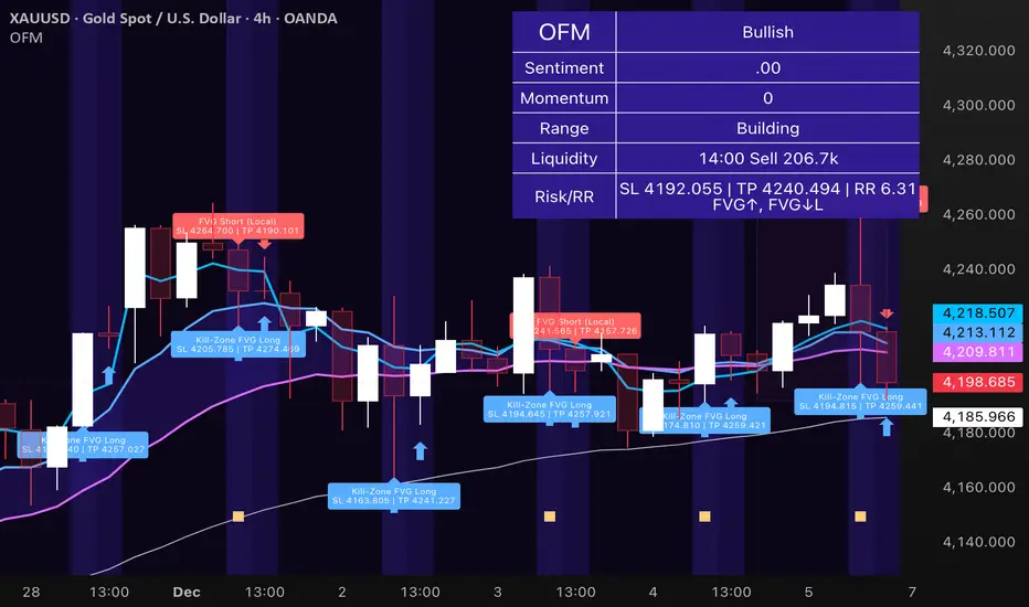
Obsidian Flux Matrix (OFM) is an open-source Pine Script v6 study that fuses social sentiment, higher timeframe trend bias, fair-value-gap detection, liquidity raids, VWAP gravitation, session profiling, and a diagnostic HUD. The layout keeps the obsidian palette so critical overlays stay readable without overwhelming a price chart.
Purpose & Scope
OFM focuses on actionable structure rather than marketing claims. It documents every driver that powers its confluence engine so reviewers understand what triggers each visual.
Core Analytical Pillars
1. Social Pulse Engine
Sentiment Webhook Feed: Accepts normalized scores (-1 to +1). Signals only arm when the EMA-smoothed value exceeds the `sentimentMin` input (0.35 by default).
Volume Confirmation: Requires local volume > 30-bar average × `volSpikeMult` (default 2.0) before sentiment flags.
EMA Cross Validation: Fast EMA 8 crossing above/below slow EMA 21 keeps momentum aligned with flow.
Momentum Alignment: Multi-timeframe momentum composite must agree (positive for longs, negative for shorts).
2. Peer Momentum Heatmap
Multi-Timeframe Blend: RSI + Stoch RSI fetched via request.security() on 1H/4H/1D by default.
Composite Scoring: Each timeframe votes +1/-1/0; totals are clamped between -3 and +3.
Intraday Readability: Configurable band thickness (1-5) so scalpers see context without losing space.
Dynamic Opacity: Stronger agreement boosts column opacity for quick bias checks.
3. Trend & Displacement Framework
Dual EMA Ribbon: Cyan/magenta ribbon highlights immediate posture.
HTF Bias: A higher-timeframe EMA (default 55 on 4H) sets macro direction.
Displacement Score: Body-to-ATR ratio (>1.4 default) detects impulses that seed FVGs or VWAP raids.
ATR Normalization: All thresholds float with volatility so the study adapts to assets and regimes.
4. Intelligent Fair Value Gap (FVG) System
Gap Detection: Three-candle logic (bullish: low > high ; bearish: high < low ) with ATR-sized minimums (0.15 × ATR default).
Overlap Prevention: Price-range checks stop redundant boxes.
Spacing Control: `fvgMinSpacing` (default 5) avoids stacking from the same impulse.
Storage Caps: Max three FVGs per side unless the user widens the limit.
Session Awareness: Kill zone filters keep taps focused on London/NY if desired.
Auto Cleanup: Boxes delete when price closes beyond their invalidation level.
5. VWAP Magnet + Liquidity Raid Engine
Session or Rolling VWAP: Toggle resets to match intraday or rolling preferences.
Equal High/Low Scanner: Looks back 20 bars by default for liquidity pools.
Displacement Filter: ATR multiplier ensures raids represent genuine liquidity sweeps.
Mean Reversion Focus: Signals fire when price displaces back toward VWAP following a raid.
6. Session Range Breakout System
Initial Balance Tracking: First N bars (15 default) define the session box.
Breakout Logic: Requires simultaneous liquidity spikes, nearby FVG activity, and supportive momentum.
Z-Score Volume Filter: >1.5σ by default to filter noisy moves.
7. Lifestyle Liquidity Scanner
Volume Z-Scores: 50-bar baseline highlights statistically significant spikes.
Smart Money Footprints: Bottom-of-chart squares color-code buy vs sell participation.
Panel Memory: HUD logs the last five raid timestamps, direction, and normalized size.
8. Risk Matrix & Diagnostic HUD
HUD Structure: Table in the top-right summarizes HTF bias, sentiment, momentum, range state, liquidity memory, and current risk references.
Signal Tags: Aggregates SPS, FVG, VWAP, Range, and Liquidity states into a compact string.
Risk Metrics: Swing-based stops (5-bar lookback) + ATR targets (1.5× default) keep risk transparent.
Signal Families & Alerts
Social Pulse (SPS): Volume-confirmed sentiment alignment; triangle markers with “SPS”.
Kill-Zone FVG: Session + HTF alignment + FVG tap; arrow markers plus SL/TP labels.
Local FVG: Captures local reversals when HTF bias has not flipped yet.
VWAP Raid: Equal-high/low raids that snap toward VWAP; “VWAP” label markers.
Range Breakout: Initial balance violations with liquidity and imbalance confirmation; circle markers.
Liquidity Spike: Z-score spikes ≥ threshold; square markers along the baseline.
Visual Design & Customization
Theme Palette: Primary background RGB (12,6,24). Accent shading RGB (26,10,48). Long accents RGB (88,174,255). Short accents RGB (219,109,255).
Stylized Candles: Optional overlay using theme colors.
Signal Toggles: Independently enable markers, heatmap, and diagnostics.
Label Spacing: Auto-spacing enforces ≥4-bar gaps to prevent text overlap.
Customization & Workflow Notes
Adjust ATR/FVG thresholds when volatility shifts.
Re-anchor sentiment to your webhook cadence; EMA smoothing (default 5) dampens noise.
Reposition the HUD by editing the `table.new` coordinates.
Use multiples of the chart timeframe for HTF requests to minimize load.
Session inputs accept exchange-local time; align them to your market.
Performance & Compliance
Pure Pine v6: Single-line statements, no `lookahead_on`.
Resource Safe: Arrays trimmed, boxes limited, `request.security` cached.
Repaint Awareness: Signals confirm on close; alerts mirror on-chart logic.
Runtime Safety: Arrays/loops guard against `na`.
Use Cases
Measure when social sentiment aligns with structure.
Plan ICT-style intraday rebalances around session-specific FVG taps.
Fade VWAP raids when displacement shows exhaustion.
Watch initial balance breaks backed by statistical volume.
Keep risk/target references anchored in ATR logic.
Signal Logic Snapshot
Social Pulse Long/Short: `sentimentEMA` gated by `sentimentMin`, `volSpike`, EMA 8/21 cross, and `momoComposite` sign agreement. Keeps hype tied to structural follow-through.
Kill-Zone FVG Long/Short: Requires session filter, HTF EMA bias alignment, and an active FVG tap (`bullFvgTap` / `bearFvgTap`). Labels include swing stops + ATR targets pulled from `swingLookback` and `liqTargetMultiple`.
Local FVG Long/Short: Uses `localBullish` / `localBearish` heuristics (EMA slope, displacement, sequential closes) to surface intraday reversals even when HTF bias has not flipped.
VWAP Raids: Detect equal-high/equal-low sweeps (`raidHigh`, `raidLow`) that revert toward `sessionVwap` or rolling VWAP when displacement exceeds `vwapAlertDisplace`.
Range Breakouts: Combine `rangeComplete`, breakout confirmation, liquidity spikes, and nearby FVG activity for statistically backed initial balance breaks.
Liquidity Spikes: Volume Z-score > `zScoreThreshold` logs direction, size, and timestamp for the HUD and optional review workflows.
Session Logic & VWAP Handling
Kill zone + NY session inputs use TradingView’s session strings; `f_inSession()` drives both visual shading and whether FVG taps are tradeable when `killZoneOnly` is true.
Session VWAP resets using cumulative price × volume sums that restart when the daily timestamp changes; rolling VWAP falls back to `ta.vwap(hlc3)` for instruments where daily resets are less relevant.
Initial balance box (`rangeBars` input) locks once complete, extends forward, and stays on chart to contextualize later liquidity raids or breakouts.
Parameter Reference
Trend: `emaFastLen`, `emaSlowLen`, `htfResolution`, `htfEmaLen`, `showEmaRibbon`, `showHtfBiasLine`.
Momentum: `tf1`, `tf2`, `tf3`, `rsiLen`, `stochLen`, `stochSmooth`, `heatmapHeight`.
Volume/Liquidity: `volLookback`, `volSpikeMult`, `zScoreLen`, `zScoreThreshold`, `equalLookback`.
VWAP & Sessions: `vwapMode`, `showVwapLine`, `vwapAlertDisplace`, `killSession`, `nySession`, `showSessionShade`, `rangeBars`.
FVG/Risk: `fvgMinTicks`, `fvgLookback`, `fvgMinSpacing`, `killZoneOnly`, `liqTargetMultiple`, `swingLookback`.
Visualization Toggles: `showSignalMarkers`, `showHeatmapBand`, `showInfoPanel`, `showStylizedCandles`.
Workflow Recipes
Kill-Zone Continuation: During the defined kill session, look for `killFvgLong` or `killFvgShort` arrows that line up with `sentimentValid` and positive `momoComposite`. Use the HUD’s risk readout to confirm SL/TP distances before entering.
VWAP Raid Fade: Outside kill zone, track `raidToVwapLong/Short`. Confirm the candle body exceeds the displacement multiplier, and price crosses back toward VWAP before considering reversions.
Range Break Monitor: After the initial balance locks, mark `rangeBreakLong/Short` circles only when the momentum band is >0 or <0 respectively and a fresh FVG box sits near price.
Liquidity Spike Review: When the HUD shows “Liquidity” timestamps, hover the plotted squares at chart bottom to see whether spikes were buy/sell oriented and if local FVGs formed immediately after.
Metadata
Author: officialjackofalltrades
Platform: TradingView (Pine Script v6)
Category: Sentiment + Liquidity Intelligence
Hope you Enjoy!
Artificialintelligence
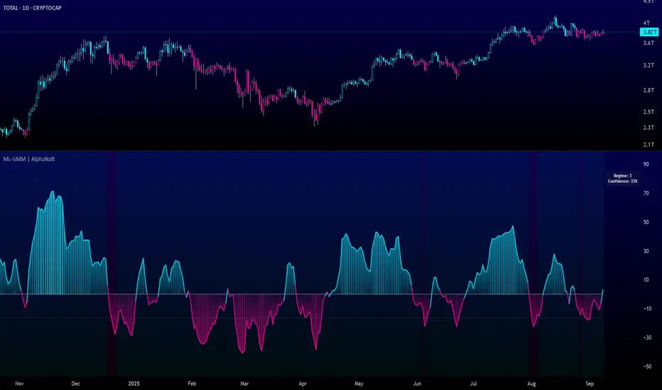
Machine Learning Gaussian Mixture Model | AlphaNattMachine Learning Gaussian Mixture Model | AlphaNatt
A revolutionary oscillator that uses Gaussian Mixture Models (GMM) with unsupervised machine learning to identify market regimes and automatically adapt momentum calculations - bringing statistical pattern recognition techniques to trading.
"Markets don't follow a single distribution - they're a mixture of different regimes. This oscillator identifies which regime we're in and adapts accordingly."
━━━━━━━━━━━━━━━━━━━━━━━━━━━━━━━━━━━━━━━━
🤖 THE MACHINE LEARNING
Gaussian Mixture Models (GMM):
Unlike K-means clustering which assigns hard boundaries, GMM uses probabilistic clustering :
Models data as coming from multiple Gaussian distributions
Each market regime is a different Gaussian component
Provides probability of belonging to each regime
More sophisticated than simple clustering
Expectation-Maximization Algorithm:
The indicator continuously learns and adapts using the E-M algorithm:
E-step: Calculate probability of current market belonging to each regime
M-step: Update regime parameters based on new data
Continuous learning without repainting
Adapts to changing market conditions
━━━━━━━━━━━━━━━━━━━━━━━━━━━━━━━━━━━━━━━━
🎯 THREE MARKET REGIMES
The GMM identifies three distinct market states:
Regime 1 - Low Volatility:
Quiet, ranging markets
Uses RSI-based momentum calculation
Reduces false signals in choppy conditions
Background: Pink tint
Regime 2 - Normal Market:
Standard trending conditions
Uses Rate of Change momentum
Balanced sensitivity
Background: Gray tint
Regime 3 - High Volatility:
Strong trends or volatility events
Uses Z-score based momentum
Captures extreme moves
Background: Cyan tint
━━━━━━━━━━━━━━━━━━━━━━━━━━━━━━━━━━━━━━━━
💡 KEY INNOVATIONS
1. Probabilistic Regime Detection:
Instead of binary regime assignment, provides probabilities:
30% Regime 1, 60% Regime 2, 10% Regime 3
Smooth transitions between regimes
No sudden indicator jumps
2. Weighted Momentum Calculation:
Combines three different momentum formulas
Weights based on regime probabilities
Automatically adapts to market conditions
3. Confidence Indicator:
Shows how certain the model is (white line)
High confidence = strong regime identification
Low confidence = transitional market state
Line transparency changes with confidence
━━━━━━━━━━━━━━━━━━━━━━━━━━━━━━━━━━━━━━━━
⚙️ PARAMETER OPTIMIZATION
Training Period (50-500):
50-100: Quick adaptation to recent conditions
100: Balanced (default)
200-500: Stable regime identification
Number of Components (2-5):
2: Simple bull/bear regimes
3: Low/Normal/High volatility (default)
4-5: More granular regime detection
Learning Rate (0.1-1.0):
0.1-0.3: Slow, stable learning
0.3: Balanced (default)
0.5-1.0: Fast adaptation
━━━━━━━━━━━━━━━━━━━━━━━━━━━━━━━━━━━━━━━━
📊 TRADING STRATEGIES
Visual Signals:
Cyan gradient: Bullish momentum
Magenta gradient: Bearish momentum
Background color: Current regime
Confidence line: Model certainty
1. Regime-Based Trading:
Regime 1 (pink): Expect mean reversion
Regime 2 (gray): Standard trend following
Regime 3 (cyan): Strong momentum trades
2. Confidence-Filtered Signals:
Only trade when confidence > 70%
High confidence = clearer market state
Avoid transitions (low confidence)
3. Adaptive Position Sizing:
Regime 1: Smaller positions (choppy)
Regime 2: Normal positions
Regime 3: Larger positions (trending)
━━━━━━━━━━━━━━━━━━━━━━━━━━━━━━━━━━━━━━━━
🚀 ADVANTAGES OVER OTHER ML INDICATORS
vs K-Means Clustering:
Soft clustering (probabilities) vs hard boundaries
Captures uncertainty and transitions
More mathematically robust
vs KNN (K-Nearest Neighbors):
Unsupervised learning (no historical labels needed)
Continuous adaptation
Lower computational complexity
vs Neural Networks:
Interpretable (know what each regime means)
No overfitting issues
Works with limited data
━━━━━━━━━━━━━━━━━━━━━━━━━━━━━━━━━━━━━━━━
📈 PERFORMANCE CHARACTERISTICS
Best Market Conditions:
Markets with clear regime shifts
Volatile to trending transitions
Multi-timeframe analysis
Cryptocurrency markets (high regime variation)
Key Strengths:
Automatically adapts to market changes
No manual parameter adjustment needed
Smooth transitions between regimes
Probabilistic confidence measure
━━━━━━━━━━━━━━━━━━━━━━━━━━━━━━━━━━━━━━━━
🔬 TECHNICAL BACKGROUND
Gaussian Mixture Models are used extensively in:
Speech recognition (Google Assistant)
Computer vision (facial recognition)
Astronomy (galaxy classification)
Genomics (gene expression analysis)
Finance (risk modeling at investment banks)
The E-M algorithm was developed at Stanford in 1977 and is one of the most important algorithms in unsupervised machine learning.
━━━━━━━━━━━━━━━━━━━━━━━━━━━━━━━━━━━━━━━━
💡 PRO TIPS
Watch regime transitions: Best opportunities often occur when regimes change
Combine with volume: High volume + regime change = strong signal
Use confidence filter: Avoid low confidence periods
Multi-timeframe: Compare regimes across timeframes
Adjust position size: Scale based on identified regime
━━━━━━━━━━━━━━━━━━━━━━━━━━━━━━━━━━━━━━━━
⚠️ IMPORTANT NOTES
Machine learning adapts but doesn't predict the future
Best used with other confirmation indicators
Allow time for model to learn (100+ bars)
Not financial advice - educational purposes
Backtest thoroughly on your instruments
━━━━━━━━━━━━━━━━━━━━━━━━━━━━━━━━━━━━━━━━
🏆 CONCLUSION
The GMM Momentum Oscillator brings institutional-grade machine learning to retail trading. By identifying market regimes probabilistically and adapting momentum calculations accordingly, it provides:
Automatic adaptation to market conditions
Clear regime identification with confidence levels
Smooth, professional signal generation
True unsupervised machine learning
This isn't just another indicator with "ML" in the name - it's a genuine implementation of Gaussian Mixture Models with the Expectation-Maximization algorithm, the same technology used in:
Google's speech recognition
Tesla's computer vision
NASA's data analysis
Wall Street risk models
"Let the machine learn the market regimes. Trade with statistical confidence."
━━━━━━━━━━━━━━━━━━━━━━━━━━━━━━━━━━━━━━━━
Developed by AlphaNatt | Machine Learning Trading Systems
Version: 1.0
Algorithm: Gaussian Mixture Model with E-M
Classification: Unsupervised Learning Oscillator
Not financial advice. Always DYOR.
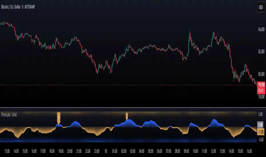
CNN Statistical Trading System [PhenLabs]📌 DESCRIPTION
An advanced pattern recognition system utilizing Convolutional Neural Network (CNN) principles to identify statistically significant market patterns and generate high-probability trading signals.
CNN Statistical Trading System transforms traditional technical analysis by applying machine learning concepts directly to price action. Through six specialized convolution kernels, it detects momentum shifts, reversal patterns, consolidation phases, and breakout setups simultaneously. The system combines these pattern detections using adaptive weighting based on market volatility and trend strength, creating a sophisticated composite score that provides both directional bias and signal confidence on a normalized -1 to +1 scale.
🚀 CONCEPTS
• Built on Convolutional Neural Network pattern recognition methodology adapted for financial markets
• Six specialized kernels detect distinct price patterns: upward/downward momentum, peak/trough formations, consolidation, and breakout setups
• Activation functions create non-linear responses with tanh-like behavior, mimicking neural network layers
• Adaptive weighting system adjusts pattern importance based on current market regime (volatility < 2% and trend strength)
• Multi-confirmation signals require CNN threshold breach (±0.65), RSI boundaries, and volume confirmation above 120% of 20-period average
🔧 FEATURES
Six-Kernel Pattern Detection:
Simultaneous analysis of upward momentum, downward momentum, peak/resistance, trough/support, consolidation, and breakout patterns using mathematically optimized convolution kernels.
Adaptive Neural Architecture:
Dynamic weight adjustment based on market volatility (ATR/Price) and trend strength (EMA differential), ensuring optimal performance across different market conditions.
Professional Visual Themes:
Four sophisticated color palettes (Professional, Ocean, Sunset, Monochrome) with cohesive design language. Default Monochrome theme provides clean, distraction-free analysis.
Confidence Band System:
Upper and lower confidence zones at 150% of threshold values (±0.975) help identify high-probability signal areas and potential exhaustion zones.
Real-Time Information Panel:
Live display of CNN score, market state with emoji indicators, net momentum, confidence percentage, and RSI confirmation with dynamic color coding based on signal strength.
Individual Feature Analysis:
Optional display of all six kernel outputs with distinct visual styles (step lines, circles, crosses, area fills) for advanced pattern component analysis.
User Guide
• Monitor CNN Score crossing above +0.65 for long signals or below -0.65 for short signals with volume confirmation
• Use confidence bands to identify optimal entry zones - signals within confidence bands carry higher probability
• Background intensity reflects signal strength - darker backgrounds indicate stronger conviction
• Enter long positions when blue circles appear above oscillator with RSI < 75 and volume > 120% average
• Enter short positions when dark circles appear below oscillator with RSI > 25 and volume confirmation
• Information panel provides real-time confidence percentage and momentum direction for position sizing decisions
• Individual feature plots allow granular analysis of specific pattern components for strategy refinement
💡Conclusion
CNN Statistical Trading System represents the evolution of technical analysis, combining institutional-grade pattern recognition with retail accessibility. The six-kernel architecture provides comprehensive market pattern coverage while adaptive weighting ensures relevance across all market conditions. Whether you’re seeking systematic entry signals or advanced pattern confirmation, this indicator delivers mathematically rigorous analysis with intuitive visual presentation.

Professional MSTI+ Trading Indicator"Professional MSTI+ Trading Indicator" is a comprehensive technical analysis tool that combines over 20 indicators to generate high-quality trading signals and assess market sentiment. The script integrates standard indicators (MACD, RSI, Bollinger Bands, Stochastic, Simple Moving Averages, and Volume Analysis) with advanced components (Squeeze Momentum, Fisher Transform, True Strength Index, Heikin-Ashi, Laguerre RSI, Hull MA) and further includes metrics such as ADX, Chaikin Money Flow, Williams %R, VWAP, and EMA for in-depth market analysis.
Key Features:
Multiple Presets for Different Trading Styles:
Choose from optimal configurations like Professional, Swing Trading, Day Trading, Scalping, or Reversal Hunter. Note that the presets may not work perfectly on all pairs, and manual calibration might be required. This flexibility allows you to fine-tune the settings to align with your unique strategies and signals.
Multi-Layered Signal Filtering:
Filters based on trend, volume, and volatility help eliminate false signals, enhancing the accuracy of market entries.
Comprehensive Fear & Greed Index:
The indicator aggregates data from RSI, volatility, momentum, trend, and volume to gauge overall market sentiment, providing an additional layer of market context.
Dynamic Information Panel:
Displays detailed status updates for each component (e.g., MACD, RSI, Laguerre RSI, TSI, Fisher Transform, Squeeze, Hull MA, etc.) along with a visual strength bar that represents the intensity of the trading signal.
Signal Generation:
Buy and sell signals are generated when a predefined number of conditions are met and confirmed over multiple bars. These signals are clearly displayed on the chart with arrows, making it easier to spot potential entry and exit points.
Alert Setup:
Built-in alert conditions allow you to receive real-time notifications when trading signals are generated, helping you stay on top of market movements.
"Professional MSTI+ Trading Indicator" is designed to enhance your trading strategy by providing a multi-faceted market analysis and an intuitive visual interface. While the presets offer a robust starting point, they may require manual calibration on certain pairs, giving you the flexibility to configure your own unique strategies and signals.

AI Adaptive Oscillator [PhenLabs]📊 Algorithmic Adaptive Oscillator
Version: PineScript™ v6
📌 Description
The AI Adaptive Oscillator is a sophisticated technical indicator that employs ensemble learning and adaptive weighting techniques to analyze market conditions. This innovative oscillator combines multiple traditional technical indicators through an AI-driven approach that continuously evaluates and adjusts component weights based on historical performance. By integrating statistical modeling with machine learning principles, the indicator adapts to changing market dynamics, providing traders with a responsive and reliable tool for market analysis.
🚀 Points of Innovation:
Ensemble learning framework with adaptive component weighting
Performance-based scoring system using directional accuracy
Dynamic volatility-adjusted smoothing mechanism
Intelligent signal filtering with cooldown and magnitude requirements
Signal confidence levels based on multi-factor analysis
🔧 Core Components
Ensemble Framework : Combines up to five technical indicators with performance-weighted integration
Adaptive Weighting : Continuous performance evaluation with automated weight adjustment
Volatility-Based Smoothing : Adapts sensitivity based on current market volatility
Pattern Recognition : Identifies potential reversal patterns with signal qualification criteria
Dynamic Visualization : Professional color schemes with gradient intensity representation
Signal Confidence : Three-tiered confidence assessment for trading signals
🔥 Key Features
The indicator provides comprehensive market analysis through:
Multi-Component Ensemble : Integrates RSI, CCI, Stochastic, MACD, and Volume-weighted momentum
Performance Scoring : Evaluates each component based on directional prediction accuracy
Adaptive Smoothing : Automatically adjusts based on market volatility
Pattern Detection : Identifies potential reversal patterns in overbought/oversold conditions
Signal Filtering : Prevents excessive signals through cooldown periods and minimum change requirements
Confidence Assessment : Displays signal strength through intuitive confidence indicators (average, above average, excellent)
🎨 Visualization
Gradient-Filled Oscillator : Color intensity reflects strength of market movement
Clear Signal Markers : Distinct bullish and bearish pattern signals with confidence indicators
Range Visualization : Clean representation of oscillator values from -6 to 6
Zero Line : Clear demarcation between bullish and bearish territory
Customizable Colors : Color schemes that can be adjusted to match your chart style
Confidence Symbols : Intuitive display of signal confidence (no symbol, +, or ++) alongside direction markers
📖 Usage Guidelines
⚙️ Settings Guide
Color Settings
Bullish Color
Default: #2b62fa (Blue)
This setting controls the color representation for bullish movements in the oscillator. The color appears when the oscillator value is positive (above zero), with intensity indicating the strength of the bullish momentum. A brighter shade indicates stronger bullish pressure.
Bearish Color
Default: #ce9851 (Amber)
This setting determines the color representation for bearish movements in the oscillator. The color appears when the oscillator value is negative (below zero), with intensity reflecting the strength of the bearish momentum. A more saturated shade indicates stronger bearish pressure.
Signal Settings
Signal Cooldown (bars)
Default: 10
Range: 1-50
This parameter sets the minimum number of bars that must pass before a new signal of the same type can be generated. Higher values reduce signal frequency and help prevent overtrading during choppy market conditions. Lower values increase signal sensitivity but may generate more false positives.
Min Change For New Signal
Default: 1.5
Range: 0.5-3.0
This setting defines the minimum required change in oscillator value between consecutive signals of the same type. It ensures that new signals represent meaningful changes in market conditions rather than minor fluctuations. Higher values produce fewer but potentially higher-quality signals, while lower values increase signal frequency.
AI Core Settings
Base Length
Default: 14
Minimum: 2
This fundamental setting determines the primary calculation period for all technical components in the ensemble (RSI, CCI, Stochastic, etc.). It represents the lookback window for each component’s base calculation. Shorter periods create a more responsive but potentially noisier oscillator, while longer periods produce smoother signals with potential lag.
Adaptive Speed
Default: 0.1
Range: 0.01-0.3
Controls how quickly the oscillator adapts to new market conditions through its volatility-adjusted smoothing mechanism. Higher values make the oscillator more responsive to recent price action but potentially more erratic. Lower values create smoother transitions but may lag during rapid market changes. This parameter directly influences the indicator’s adaptiveness to market volatility.
Learning Lookback Period
Default: 150
Minimum: 10
Determines the historical data range used to evaluate each ensemble component’s performance and calculate adaptive weights. This setting controls how far back the AI “learns” from past performance to optimize current signals. Longer periods provide more stable weight distribution but may be slower to adapt to regime changes. Shorter periods adapt more quickly but may overreact to recent anomalies.
Ensemble Size
Default: 5
Range: 2-5
Specifies how many technical components to include in the ensemble calculation.
Understanding The Interaction Between Settings
Base Length and Learning Lookback : The base length determines the reactivity of individual components, while the lookback period determines how their weights are adjusted. These should be balanced according to your timeframe - shorter timeframes benefit from shorter base lengths, while the lookback should generally be 10-15 times the base length for optimal learning.
Adaptive Speed and Signal Cooldown : These settings control sensitivity from different angles. Increasing adaptive speed makes the oscillator more responsive, while reducing signal cooldown increases signal frequency. For conservative trading, keep adaptive speed low and cooldown high; for aggressive trading, do the opposite.
Ensemble Size and Min Change : Larger ensembles provide more stable signals, allowing for a lower minimum change threshold. Smaller ensembles might benefit from a higher threshold to filter out noise.
Understanding Signal Confidence Levels
The indicator provides three distinct confidence levels for both bullish and bearish signals:
Average Confidence (▲ or ▼) : Basic signal that meets the minimum pattern and filtering criteria. These signals indicate potential reversals but with moderate confidence in the prediction. Consider using these as initial alerts that may require additional confirmation.
Above Average Confidence (▲+ or ▼+) : Higher reliability signal with stronger underlying metrics. These signals demonstrate greater consensus among the ensemble components and/or stronger historical performance. They offer increased probability of successful reversals and can be traded with less additional confirmation.
Excellent Confidence (▲++ or ▼++) : Highest quality signals with exceptional underlying metrics. These signals show strong agreement across oscillator components, excellent historical performance, and optimal signal strength. These represent the indicator’s highest conviction trade opportunities and can be prioritized in your trading decisions.
Confidence assessment is calculated through a multi-factor analysis including:
Historical performance of ensemble components
Degree of agreement between different oscillator components
Relative strength of the signal compared to historical thresholds
✅ Best Use Cases:
Identify potential market reversals through oscillator extremes
Filter trade signals based on AI-evaluated component weights
Monitor changing market conditions through oscillator direction and intensity
Confirm trade signals from other indicators with adaptive ensemble validation
Detect early momentum shifts through pattern recognition
Prioritize trading opportunities based on signal confidence levels
Adjust position sizing according to signal confidence (larger for ++ signals, smaller for standard signals)
⚠️ Limitations
Requires sufficient historical data for accurate performance scoring
Ensemble weights may lag during dramatic market condition changes
Higher ensemble sizes require more computational resources
Performance evaluation quality depends on the learning lookback period length
Even high confidence signals should be considered within broader market context
💡 What Makes This Unique
Adaptive Intelligence : Continuously adjusts component weights based on actual performance
Ensemble Methodology : Combines strength of multiple indicators while minimizing individual weaknesses
Volatility-Adjusted Smoothing : Provides appropriate sensitivity across different market conditions
Performance-Based Learning : Utilizes historical accuracy to improve future predictions
Intelligent Signal Filtering : Reduces noise and false signals through sophisticated filtering criteria
Multi-Level Confidence Assessment : Delivers nuanced signal quality information for optimized trading decisions
🔬 How It Works
The indicator processes market data through five main components:
Ensemble Component Calculation :
Normalizes traditional indicators to consistent scale
Includes RSI, CCI, Stochastic, MACD, and volume components
Adapts based on the selected ensemble size
Performance Evaluation :
Analyzes directional accuracy of each component
Calculates continuous performance scores
Determines adaptive component weights
Oscillator Integration :
Combines weighted components into unified oscillator
Applies volatility-based adaptive smoothing
Scales final values to -6 to 6 range
Signal Generation :
Detects potential reversal patterns
Applies cooldown and magnitude filters
Generates clear visual markers for qualified signals
Confidence Assessment :
Evaluates component agreement, historical accuracy, and signal strength
Classifies signals into three confidence tiers (average, above average, excellent)
Displays intuitive confidence indicators (no symbol, +, ++) alongside direction markers
💡 Note:
The AI Adaptive Oscillator performs optimally when used with appropriate timeframe selection and complementary indicators. Its adaptive nature makes it particularly valuable during changing market conditions, where traditional fixed-weight indicators often lose effectiveness. The ensemble approach provides a more robust analysis by leveraging the collective intelligence of multiple technical methodologies. Pay special attention to the signal confidence indicators to optimize your trading decisions - excellent (++) signals often represent the most reliable trade opportunities.
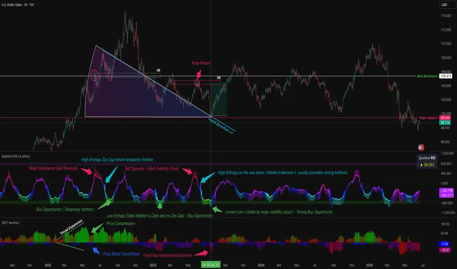
QT RSI [ W.ARITAS ]The QT RSI is an innovative technical analysis indicator designed to enhance precision in market trend identification and decision-making. Developed using advanced concepts in quantum mechanics, machine learning (LSTM), and signal processing, this indicator provides actionable insights for traders across multiple asset classes, including stocks, crypto, and forex.
Key Features:
Dynamic Color Gradient: Visualizes market conditions for intuitive interpretation:
Green: Strong buy signal indicating bullish momentum.
Blue: Neutral or observation zone, suggesting caution or lack of a clear trend.
Red: Strong sell signal indicating bearish momentum.
Quantum-Enhanced RSI: Integrates adaptive energy levels, dynamic smoothing, and quantum oscillators for precise trend detection.
Hybrid Machine Learning Model: Combines LSTM neural networks and wavelet transforms for accurate prediction and signal refinement.
Customizable Settings: Includes advanced parameters for dynamic thresholds, sensitivity adjustment, and noise reduction using Kalman and Jurik filters.
How to Use:
Interpret the Color Gradient:
Green Zone: Indicates bullish conditions and potential buy opportunities. Look for upward momentum in the RSI plot.
Blue Zone: Represents a neutral or consolidation phase. Monitor the market for trend confirmation.
Red Zone: Indicates bearish conditions and potential sell opportunities. Look for downward momentum in the RSI plot.
Follow Overbought/Oversold Boundaries:
Use the upper and lower RSI boundaries to identify overbought and oversold conditions.
Leverage Advanced Filtering:
The smoothed signals and quantum oscillator provide a robust framework for filtering false signals, making it suitable for volatile markets.
Application: Ideal for traders and analysts seeking high-precision tools for:
Identifying entry and exit points.
Detecting market reversals and momentum shifts.
Enhancing algorithmic trading strategies with cutting-edge analytics.
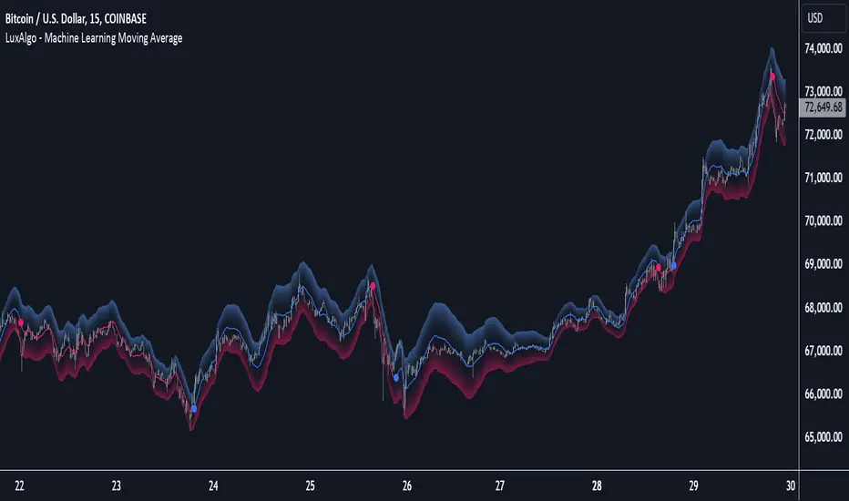
Machine Learning Moving Average [LuxAlgo]The Machine Learning Moving Average (MLMA) is a responsive moving average making use of the weighting function obtained Gaussian Process Regression method. Characteristic such as responsiveness and smoothness can be adjusted by the user from the settings.
The moving average also includes bands, used to highlight possible reversals.
🔶 USAGE
The Machine Learning Moving Average smooths out noisy variations from the price, directly estimating the underlying trend in the price.
A higher "Window" setting will return a longer-term moving average while increasing the "Forecast" setting will affect the responsiveness and smoothness of the moving average, with higher positive values returning a more responsive moving average and negative values returning a smoother but less responsive moving average.
Do note that an excessively high "Forecast" setting will result in overshoots, with the moving average having a poor fit with the price.
The moving average color is determined according to the estimated trend direction based on the bands described below, shifting to blue (default) in an uptrend and fushia (default) in downtrends.
The upper and lower extremities represent the range within which price movements likely fluctuate.
Signals are generated when the price crosses above or below the band extremities, with turning points being highlighted by colored circles on the chart.
🔶 SETTINGS
Window: Calculation period of the moving average. Higher values yield a smoother average, emphasizing long-term trends and filtering out short-term fluctuations.
Forecast: Sets the projection horizon for Gaussian Process Regression. Higher values create a more responsive moving average but will result in more overshoots, potentially worsening the fit with the price. Negative values will result in a smoother moving average.
Sigma: Controls the standard deviation of the Gaussian kernel, influencing weight distribution. Higher Sigma values return a longer-term moving average.
Multiplicative Factor: Adjusts the upper and lower extremity bounds, with higher values widening the bands and lowering the amount of returned turning points.
🔶 RELATED SCRIPTS
Machine-Learning-Gaussian-Process-Regression
SuperTrend-AI-Clustering
Machine Learning using Neural Networks | EducationalThe script provided is a comprehensive illustration of how to implement and execute a simplistic Neural Network (NN) on TradingView using PineScript.
It encompasses the entire workflow from data input, weight initialization, implicit neuron calculation, feedforward computation, backpropagation for weight adjustments, generating predictions, to visualizing the Mean Squared Error (MSE) Loss Curve for monitoring the training phase.
In the visual example above, you can see that the prediction is not aligned with the actual value. This is intentional for demonstrative purposes, and by incrementing the Epochs or Learning Rate, you will see these two values converge as the accuracy increases.
Hyperparameters:
Learning Rate, Epochs, and the choice between Simple Backpropagation and a verbose version are declared as script inputs, allowing users to tailor the training process.
Initialization:
Random initialization of weight matrices (w1, w2) is performed to ensure asymmetry, promoting effective gradient updates. A seed is added for reproducibility.
Utility Functions:
Functions for matrix randomization, sigmoid activation, MSE loss calculation, data normalization, and standardization are defined to streamline the computation process.
Neural Network Computation:
The feedforward function computes the hidden and output layer values given the input.
Two variants of the backpropagation function are provided for weight adjustment, with one offering a more verbose step-by-step computation of gradients.
A wrapper train_nn function iterates through epochs, performing feedforward, loss computation, and backpropagation in each epoch while logging and collecting loss values.
Training Invocation:
The input data is prepared by normalizing it to a value between 0 and 1 using the maximum standardized value, and the training process is invoked only on the last confirmed bar to preserve computational resources.
Output Forecasting and Visualization:
Post training, the NN's output (predicted price) is computed, standardized and visualized alongside the actual price on the chart.
The MSE loss between the predicted and actual prices is visualized, providing insight into the prediction accuracy.
Optionally, the MSE Loss Curve is plotted on the chart, illustrating the loss trajectory through epochs, assisting in understanding the training performance.
Customizable Visualization:
Various inputs control visualization aspects like Chart Scaling, Chart Horizontal Offset, and Chart Vertical Offset, allowing users to adapt the visualization to their preference.
-------------------------------------------------------
The following is this Neural Network structure, consisting of one hidden layer, with two hidden neurons.
Through understanding the steps outlined in my code, one should be able to scale the NN in any way they like, such as changing the input / output data and layers to fit their strategy ideas.
Additionally, one could forgo the backpropagation function, and load their own trained weights into the w1 and w2 matrices, to have this code run purely for inference.
-------------------------------------------------------
While this demonstration does create a “prediction”, it is on historical data. The purpose here is educational, rather than providing a ready tool for non-programmer consumers.
Normally in Machine Learning projects, the training process would be split into two segments, the Training and the Validation parts. For the purpose of conveying the core concept in a concise and non-repetitive way, I have foregone the Validation part. However, it is merely the application of your trained network on new data (feedforward), and monitoring the loss curve.
Essentially, checking the accuracy on “unseen” data, while training it on “seen” data.
-------------------------------------------------------
I hope that this code will help developers create interesting machine learning applications within the Tradingview ecosystem.
