BTC 5 min SHBHilalimSB A Wedding Gift 🌙
What is HilalimSB🌙?
First of all, as mentioned in the title, HilalimSB is a wedding gift.
HilalimSB - Revealing the Secrets of the Trend
HilalimSB is a powerful indicator designed to help investors analyze market trends and optimize trading strategies. Designed to uncover the secrets at the heart of the trend, HilalimSB stands out with its unique features and impressive algorithm.
Hilalim Algorithm and Fixed ATR Value:
HilalimSB is equipped with a special algorithm called "Hilalim" to detect market trends. This algorithm can delve into the depths of price movements to determine the direction of the trend and provide users with the ability to predict future price movements. Additionally, HilalimSB uses its own fixed Average True Range (ATR) value. ATR is an indicator that measures price movement volatility and is often used to determine the strength of a trend. The fixed ATR value of HilalimSB has been tested over long periods and its reliability has been proven. This allows users to interpret the signals provided by the indicator more reliably.
ATR Calculation Steps
1.True Range Calculation:
+ The True Range (TR) is the greatest of the following three values:
1. Current high minus current low
2. Current high minus previous close (absolute value)
3. Current low minus previous close (absolute value)
2.Average True Range (ATR) Calculation:
-The initial ATR value is calculated as the average of the TR values over a specified period
(typically 14 periods).
-For subsequent periods, the ATR is calculated using the following formula:
ATRt=(ATRt−1×(n−1)+TRt)/n
Where:
+ ATRt is the ATR for the current period,
+ ATRt−1 is the ATR for the previous period,
+ TRt is the True Range for the current period,
+ n is the number of periods.
Pine Script to Calculate ATR with User-Defined Length and Multiplier
Here is the Pine Script code for calculating the ATR with user-defined X length and Y multiplier:
//@version=5
indicator("Custom ATR", overlay=false)
// User-defined inputs
X = input.int(14, minval=1, title="ATR Period (X)")
Y = input.float(1.0, title="ATR Multiplier (Y)")
// True Range calculation
TR1 = high - low
TR2 = math.abs(high - close )
TR3 = math.abs(low - close )
TR = math.max(TR1, math.max(TR2, TR3))
// ATR calculation
ATR = ta.rma(TR, X)
// Apply multiplier
customATR = ATR * Y
// Plot the ATR value
plot(customATR, title="Custom ATR", color=color.blue, linewidth=2)
This code can be added as a new Pine Script indicator in TradingView, allowing users to calculate and display the ATR on the chart according to their specified parameters.
HilalimSB's Distinction from Other ATR Indicators
HilalimSB emerges with its unique Average True Range (ATR) value, presenting itself to users. Equipped with a proprietary ATR algorithm, this indicator is released in a non-editable form for users. After meticulous testing across various instruments with predetermined period and multiplier values, it is made available for use.
ATR is acknowledged as a critical calculation tool in the financial sector. The ATR calculation process of HilalimSB is conducted as a result of various research efforts and concrete data-based computations. Therefore, the HilalimSB indicator is published with its proprietary ATR values, unavailable for modification.
The ATR period and multiplier values provided by HilalimSB constitute the fundamental logic of a trading strategy. This unique feature aids investors in making informed decisions.
Visual Aesthetics and Clear Charts:
HilalimSB provides a user-friendly interface with clear and impressive graphics. Trend changes are highlighted with vibrant colors and are visually easy to understand. You can choose colors based on eye comfort, allowing you to personalize your trading screen for a more enjoyable experience. While offering a flexible approach tailored to users' needs, HilalimSB also promises an aesthetic and professional experience.
Strong Signals and Buy/Sell Indicators:
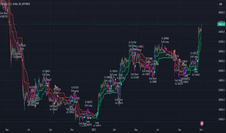
After completing test operations, HilalimSB produces data at various time intervals. However, we would like to emphasize to users that based on our studies, it provides the best signals in 1-hour chart data. HilalimSB produces strong signals to identify trend reversals. Buy or sell points are clearly indicated, allowing users to develop and implement trading strategies based on these signals.
For example, let's imagine you wanted to open a position on BTC on 2023.11.02. You are aware that you need to calculate which of the buying or selling transactions would be more profitable. You need support from various indicators to open a position. Based on the analysis and calculations it has made from the data it contains, HilalimSB would have detected that the graph is more suitable for a selling position, and by producing a sell signal at the most ideal selling point at 08:00 on 2023.11.02 (UTC+3 Istanbul), it would have informed you of the direction the graph would follow, allowing you to benefit positively from a 2.56% decline.
Technology and Innovation:
HilalimSB aims to enhance the trading experience using the latest technology. With its innovative approach, it enables users to discover market opportunities and support their decisions. Thus, investors can make more informed and successful trades. Real-Time Data Analysis: HilalimSB analyzes market data in real-time and identifies updated trends instantly. This allows users to make more informed trading decisions by staying informed of the latest market developments. Continuous Update and Improvement: HilalimSB is constantly updated and improved. New features are added and existing ones are enhanced based on user feedback and market changes. Thus, HilalimSB always aims to provide the latest technology and the best user experience.
Social Order and Intrinsic Motivation:
Negative trends such as widespread illegal gambling and uncontrolled risk-taking can have adverse financial effects on society. The primary goal of HilalimSB is to counteract these negative trends by guiding and encouraging users with data-driven analysis and calculable investment systems. This allows investors to trade more consciously and safely.
What is BTC 5 min ☆SHB Strategy🌙?
BTC 5 min ☆SHB Strategy is a strategy supported by the HilalimSB algorithm created by the creator of HilalimSB. It automatically opens trades based on the data it receives, maintaining trades with its uniquely defined take profit and stop loss levels, and automatically closes trades when necessary. It stands out in the TradingView world with its unique take profit and stop loss markings. BTC 5 min ☆SHB Strategy is close to users' initiatives and is a strategy suitable for 5-minute trades and scalp operations developed on BTC.
What does the BTC 5 min ☆SHB Strategy target?
The primary goal of BTC 5 min ☆SHB Strategy is to close trades made by traders in short timeframes as profitably as possible and to determine the most effective trading points in low time periods, considering the commission rates of various brokerage firms. BTC 5 min ☆SHB Strategy is one of the rare profitable strategies released in short timeframes, with its useful interface, in addition to existing strategies in the markets. After extensive backtesting over a long period and achieving above-average success, BTC 5 min ☆SHB Strategy was decided to be released. Following the completion of test procedures under market conditions, it was presented to users with the unique visual effects of ☆SB.
BTC 5 min ☆SHB Strategy and Heikin Ashi
BTC 5 min ☆SHB Strategy produces data in Heikin-Ashi chart types, but since Heikin-Ashi chart types have their own calculation method, BTC 5 min ☆SHB Strategy has been published in a way that cannot produce data in this chart type due to BTC 5 min ☆SHB Strategy's ideology of appealing to all types of users, and any confusion that may arise is prevented in this way. Heikin-Ashi chart types, especially in short time intervals, carry significant risks considering the unique calculation methods involved. Thus, the possibility of being misled by the coder and causing financial losses has been completely eliminated. After the necessary conditions determined by the creator of BTC 5 min ☆SHB are met, BTC 5 min ☆SHB Heikin-Ashi will be shared exclusively with invited users only, upon request, to users who request an invitation.
Key Features:
+HilalimSHB Algorithm: This algorithm uses a dynamic ATR-based trend-following mechanism to identify the current market trend. The strategy detects trend reversals and takes positions accordingly.
+Heikin Ashi Compatibility: The strategy is optimized to work only with standard candlestick charts and automatically deactivates when Heikin Ashi charts are in use, preventing false signals.
+Advanced Chart Enhancements: The strategy offers clear graphical markers for buy/sell signals. Candlesticks are automatically colored based on trend direction, making market trends easier to follow.
Strategy Parameters:
+Take Profit (%): Defines the target price level for closing a position and automates profit-taking. The fixed value is set at 2%.
+Stop Loss (%): Specifies the stop-loss level to limit losses. The fixed value is set at 3%.
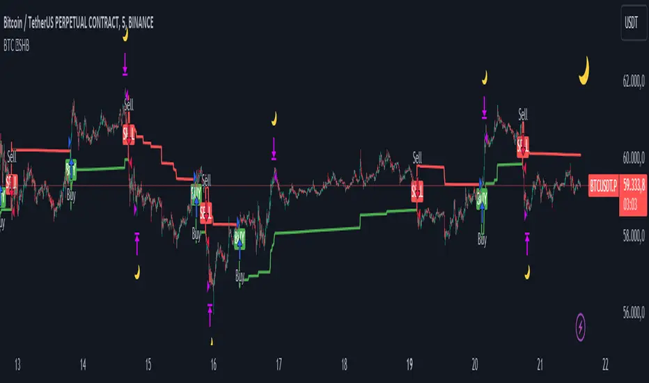
The shared image is a 5-minute chart of BTCUSDC.P with a fixed take profit value of 2% and a fixed stop loss value of 3%. The trades are opened with a commission rate of 0.063% set for the USDT trading pair on Binance.🌙
Forecasting
Fibonacci Trend Reversal StrategyIntroduction
This publication introduces the " Fibonacci Retracement Trend Reversal Strategy, " tailored for traders aiming to leverage shifts in market momentum through advanced trend analysis and risk management techniques. This strategy is designed to pinpoint potential reversal points, optimizing trading opportunities.
Overview
The strategy leverages Fibonacci retracement levels derived from @IMBA_TRADER's lance Algo to identify potential trend reversals. It's further enhanced by a method called " Trend Strength Over Time " (TSOT) (by @federalTacos5392b), which utilizes percentile rankings of price action to measure trend strength. This also has implemented Dynamic SL finder by utilizing @veryfid's ATR Stoploss Finder which works pretty well
Indicators:
Fibonacci Retracement Levels : Identifies critical reversal zones at 23.6%, 50%, and 78.6% levels.
TSOT (Trend Strength Over Time) : Employs percentile rankings across various timeframes to gauge the strength and direction of trends, aiding in the confirmation of Fibonacci-based signals.
ATR (Average True Range) : Implements dynamic stop-loss settings for both long and short positions, enhancing trade security.
Strategy Settings :
- Sensitivity: Set default at 18, adjustable for more frequent or sparse signals based on market volatility.
- ATR Stop Loss Finder: Multiplier set at 3.5, applying the ATR value to determine stop losses dynamically.
- ATR Length: Default set to 14 with RMA smoothing.
- TSOT Settings: Hard-coded to identify percentile ranks, with no user-adjustable inputs due to its intrinsic calculation method.
Trade Direction Options : Configurable to support long, short, or both directions, adaptable to the trader's market assessment.
Entry Conditions :
- Long Entry: Triggered when the price surpasses the mid Fibonacci level (50%) with a bullish TSOT signal.
- Short Entry: Activated when the price falls below the mid Fibonacci level with a bearish TSOT indication.
Exit Conditions :
- Employs ATR-based dynamic stop losses, calibrated according to current market volatility, ensuring effective risk management.
Strategy Execution :
- Risk Management: Features adjustable risk-reward settings and enables partial take profits by default to systematically secure gains.
- Position Reversal: Includes an option to reverse positions based on new TSOT signals, improving the strategy's responsiveness to evolving market conditions.
The strategy is optimized for the BYBIT:WIFUSDT.P market on a scalping (5-minute) timeframe, using the default settings outlined above.
I spent a lot of time creating the dynamic exit strategies for partially taking profits and reversing positions so please make use of those and feel free to adjust the settings, tool tips are also provided.
For Developers: this is published as open-sourced code so that developers can learn something especially on dynamic exits and partial take profits!
Good Luck!
Disclaimer
This strategy is shared for educational purposes and must be thoroughly tested under diverse market conditions. Past performance does not guarantee future results. Traders are advised to integrate this strategy with other analytical tools and tailor it to specific market scenarios. I was only sharing what I've crafted while strategizing over a Solana Meme Coin.

Spot Martingale KuCoin - The Quant ScienceINTRODUCTION
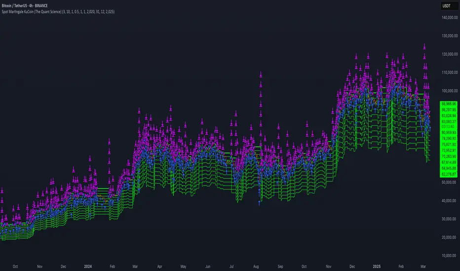
Backtesting software of the Spot Martingale algorithm offered by the KuCoin exchange.
This script replicates the logic used by the KuCoin bot and is useful for analyzing strategy on any cryptocurrency historical series.
It's not intended as an automatic trading algorithm and does not offer the possibility of automatic order execution.
The trader will use this software exclusively to research the best parameters with which to work on KuCoin.
LOGIC OF EXECUTION
The execution of orders is composed as follows:
1) Start Martingale: initial order
2) Martingale-Number: orders following Start Martingale
(A) The software is designed and developed to replicate trading without taking into account technical indicators or particular market conditions. The Initial Order (Start Martingale) will be executed immediately the close of the previous Martingale when the balance of market orders is zero. It will use the capital set in the Properties section for the initial order.
(B) After the first order, the software will open new orders as the price decreases. For orders following Start Martingale, the initial capital, multiplier, and number of orders in the exponential growth context are considered. The multiplier is the factor that determines the proportional increase in capital with each new order. The number of orders, indicates how many times the multiplier is applied to increase the investment.
Example
To find out the capital used in Martingale order number 5, with a Multiple For Position Increase equal to 2 and a starting capital of $100, the formula will be as follows:
Martingale Order = ($100 * (2 * 2 * 2 * 2 * 2)) = $100 * 32 = $3.200
(C) A multiplier is used for each new order that will increase the quantity purchased.
(D) All previously open orders are closed once the take profit is reached.
USER MANUAL
The user interface consists of two main sections:
1. Settings
Percentage Drop for Position Increase (0.1-15%) : percentage distance between Martingale orders. For example, if you set 5% each new order will be opened after a 5% price decrease from the previous one.
Max Position Increases (1-15) : number of Martingale orders to be executed after Start Martingale. For example, if you set 10, up to10 orders will be opened after Start Martingale.
Multiple For Position Increase (1-2x) : capital multiplier. For example, if you set 2 each for each new order, the capital involved will be doubled, order by order.
Take Profit Percentage (0.5-1000%) : percentage take profit, calculated on the average entry price.
2. Date Range Backtesting
The Date Range Backtesting section adjusts the analysis period. The user can easily adjust the UI parameters, and automatically the software will update the data.
LIMITATIONS OF THE MODEL
Although the Martingale model is widely used in position management, even this model has limitations and is subject to real risks during particular market conditions. Knowing these conditions will help you understand which asset is best to use the strategy on.
The main risks in adopting this automatic strategy are 2:
1) The price falls below our last order.
It happens during periods of strong bear-market in which the price collapses abruptly without experiencing any pullback. In this case the algorithm will enter a drawdown phase and the strategy will become a loser. The trader will then have to consider whether to wait for a price recovery or to incur a loss by manually closing the algorithm.
2) The price increases quickly.
It happens during periods of strong bull-market in which the price rises abruptly without experiencing any pullback. In this case the algorithm will not optimize order execution, working only with Start Martingale in the vast majority of trades. Given the exponential nature of the investment, the algorithm will in this case generate a profit that is always less than that of the reference market.
The best market conditions to use this strategy are characterized by high volatility such as correction phases during a bull run and/or markets that exhibit sideways price trends (such as areas of accumulation or congestion where price will generate many false signals).
FEATURES
This script was developed by including features to optimize the user experience.
Includes a dashboard at launch that allows the user to intuitively enter backtesting parameters.
Includes graphical indicator that helps the user analyze the behavior of the strategy.
Includes a date period backtesting feature that allows the user to adjust and choose custom historical periods.
DISCLAIMER
This script was released using parameters researched solely for the BTC/USDT pair, 4H timeframe, traded on the KuCoin Exchange (2017-present). Do not consider this combination of parameters as universal and usable on all assets and timeframes.
Bitcoin 5A Strategy@LilibtcIn our long-term strategy, we have deeply explored the key factors influencing the price of Bitcoin. By precisely calculating the correlation between these factors and the price of Bitcoin, we found that they are closely linked to the value of Bitcoin. To more effectively predict the fair price of Bitcoin, we have built a predictive model and adjusted our investment strategy accordingly based on this model. In practice, the prediction results of this model correspond quite high with actual values, fully demonstrating its reliability in predicting price fluctuations.
When the future is uncertain and the outlook is unclear, people often choose to hold back and avoid risks, or even abandon their original plans. However, the prediction of Bitcoin is full of challenges, but we have taken the first step in exploring.
Table of contents:
Usage Guide
Step 1: Identify the factors that have the greatest impact on Bitcoin price
Step 2: Build a Bitcoin price prediction model
Step 3: Find indicators for warning of bear market bottoms and bull market tops
Step 4: Predict Bitcoin Price in 2025
Step 5: Develop a Bitcoin 5A strategy
Step 6: Verify the performance of the Bitcoin 5A strategy
Usage Restrictions
🦮Usage Guide:
1. On the main interface, modify the code, find the BTCUSD trading pair, and select the BITSTAMP exchange for trading.
2. Set the time period to the daily chart.
3. Select a logarithmic chart in the chart type to better identify price trends.
4. In the strategy settings, adjust the options according to personal needs, including language, display indicators, display strategies, display performance, display optimizations, sell alerts, buy prompts, opening days, backtesting start year, backtesting start month, and backtesting start date.
🏃Step 1: Identify the factors that have the greatest impact on Bitcoin price
📖Correlation Coefficient: A mathematical concept for measuring influence
In order to predict the price trend of Bitcoin, we need to delve into the factors that have the greatest impact on its price. These factors or variables can be expressed in mathematical or statistical correlation coefficients. The correlation coefficient is an indicator of the degree of association between two variables, ranging from -1 to 1. A value of 1 indicates a perfect positive correlation, while a value of -1 indicates a perfect negative correlation.
For example, if the price of corn rises, the price of live pigs usually rises accordingly, because corn is the main feed source for pig breeding. In this case, the correlation coefficient between corn and live pig prices is approximately 0.3. This means that corn is a factor affecting the price of live pigs. On the other hand, if a shooter's performance improves while another shooter's performance deteriorates due to increased psychological pressure, we can say that the former is a factor affecting the latter's performance.
Therefore, in order to identify the factors that have the greatest impact on the price of Bitcoin, we need to find the factors with the highest correlation coefficients with the price of Bitcoin. If, through the analysis of the correlation between the price of Bitcoin and the data on the chain, we find that a certain data factor on the chain has the highest correlation coefficient with the price of Bitcoin, then this data factor on the chain can be identified as the factor that has the greatest impact on the price of Bitcoin. Through calculation, we found that the 🔵number of Bitcoin blocks is one of the factors that has the greatest impact on the price of Bitcoin. From historical data, it can be clearly seen that the growth rate of the 🔵number of Bitcoin blocks is basically consistent with the movement direction of the price of Bitcoin. By analyzing the past ten years of data, we obtained a daily correlation coefficient of 0.93 between the number of Bitcoin blocks and the price of Bitcoin.
🏃Step 2: Build a Bitcoin price prediction model
📖Predictive Model: What formula is used to predict the price of Bitcoin?
Among various prediction models, the linear function is the preferred model due to its high accuracy. Take the standard weight as an example, its linear function graph is a straight line, which is why we choose the linear function model. However, the growth rate of the price of Bitcoin and the number of blocks is extremely fast, which does not conform to the characteristics of the linear function. Therefore, in order to make them more in line with the characteristics of the linear function, we first take the logarithm of both. By observing the logarithmic graph of the price of Bitcoin and the number of blocks, we can find that after the logarithm transformation, the two are more in line with the characteristics of the linear function. Based on this feature, we choose the linear regression model to establish the prediction model.
From the graph below, we can see that the actual red and green K-line fluctuates around the predicted blue and 🟢green line. These predicted values are based on fundamental factors of Bitcoin, which support its value and reflect its reasonable value. This picture is consistent with the theory proposed by Marx in "Das Kapital" that "prices fluctuate around values."
The predicted logarithm of the market cap of Bitcoin is calculated through the model. The specific calculation formula of the Bitcoin price prediction value is as follows:
btc_predicted_marketcap = math.exp(btc_predicted_marketcap_log)
btc_predicted_price = btc_predicted_marketcap / btc_supply
🏃Step 3: Find indicators for early warning of bear market bottoms and bull market tops
📖Warning Indicator: How to Determine Whether the Bitcoin Price has Reached the Bear Market Bottom or the Bull Market Top?
By observing the Bitcoin price logarithmic prediction chart mentioned above, we notice that the actual price often falls below the predicted value at the bottom of a bear market; during the peak of a bull market, the actual price exceeds the predicted price. This pattern indicates that the deviation between the actual price and the predicted price can serve as an early warning signal. When the 🔴 Bitcoin price deviation is very low, as shown by the chart with 🟩green background, it usually means that we are at the bottom of the bear market; Conversely, when the 🔴 Bitcoin price deviation is very high, the chart with a 🟥red background indicates that we are at the peak of the bull market.
This pattern has been validated through six bull and bear markets, and the deviation value indeed serves as an early warning signal, which can be used as an important reference for us to judge market trends.
🏃Step 4:Predict Bitcoin Price in 2025
📖Price Upper Limit
According to the data calculated on February 25, 2024, the 🟠upper limit of the Bitcoin price is $194,287, which is the price ceiling of this bull market. The peak of the last bull market was on November 9, 2021, at $68,664. The bull-bear market cycle is 4 years, so the highest point of this bull market is expected in 2025. That is where you should sell the Bitcoin. and the upper limit of the Bitcoin price will exceed $190,000. The closing price of Bitcoin on February 25, 2024, was $51,729, with an expected increase of 2.7 times.
🏃Step 5: Bitcoin 5A Strategy Formulation
📖Strategy: When to buy or sell, and how many to choose?
We introduce the Bitcoin 5A strategy. This strategy requires us to generate trading signals based on the critical values of the warning indicators, simulate the trades, and collect performance data for evaluation. In the Bitcoin 5A strategy, there are three key parameters: buying warning indicator, batch trading days, and selling warning indicator. Batch trading days are set to ensure that we can make purchases in batches after the trading signal is sent, thus buying at a lower price, selling at a higher price, and reducing the trading impact cost.
In order to find the optimal warning indicator critical value and batch trading days, we need to adjust these parameters repeatedly and perform backtesting. Backtesting is a method established by observing historical data, which can help us better understand market trends and trading opportunities.
Specifically, we can find the key trading points by watching the Bitcoin price log and the Bitcoin price deviation chart. For example, on August 25, 2015, the 🔴 Bitcoin price deviation was at its lowest value of -1.11; on December 17, 2017, the 🔴 Bitcoin price deviation was at its highest value at the time, 1.69; on March 16, 2020, the 🔴 Bitcoin price deviation was at its lowest value at the time, -0.91; on March 13, 2021, the 🔴 Bitcoin price deviation was at its highest value at the time, 1.1; on December 31, 2022, the 🔴 Bitcoin price deviation was at its lowest value at the time, -1.
To ensure that all five key trading points generate trading signals, we set the warning indicator Bitcoin price deviation to the larger of the three lowest values, -0.9, and the smallest of the two highest values, 1. Then, we buy when the warning indicator Bitcoin price deviation is below -0.9, and sell when it is above 1.
In addition, we set the batch trading days as 25 days to implement a strategy that averages purchases and sales. Within these 25 days, we will invest all funds into the market evenly, buying once a day. At the same time, we also sell positions at the same pace, selling once a day.
📖Adjusting the threshold: a key step to optimizing trading strategy
Adjusting the threshold is an indispensable step for better performance. Here are some suggestions for adjusting the batch trading days and critical values of warning indicators:
• Batch trading days: Try different days like 25 to see how it affects overall performance.
• Buy and sell critical values for warning indicators: iteratively fine-tune the buy threshold value of -0.9 and the sell threshold value of 1 exhaustively to find the best combination of threshold values.
Through such careful adjustments, we may find an optimized approach with a lower maximum drawdown rate (e.g., 11%) and a higher cumulative return rate for closed trades (e.g., 474 times). The chart below is a backtest optimization chart for the Bitcoin 5A strategy, providing an intuitive display of strategy adjustments and optimizations.
In this way, we can better grasp market trends and trading opportunities, thereby achieving a more robust and efficient trading strategy.
🏃Step 6: Validating the performance of the Bitcoin 5A Strategy
📖Model interpretability validation: How to explain the Bitcoin price model?
The interpretability of the model is represented by the coefficient of determination R squared, which reflects the degree of match between the predicted value and the actual value. I divided all the historical data from August 18, 2015 into two groups, and used the data from August 18, 2011 to August 18, 2015 as training data to generate the model. The calculation result shows that the coefficient of determination R squared during the 2011-2015 training period is as high as 0.81, which shows that the interpretability of this model is quite high. From the Bitcoin price logarithmic prediction chart in the figure below, we can see that the deviation between the predicted value and the actual value is not far, which means that most of the predicted values can explain the actual value well.
The calculation formula for the coefficient of determination R squared is as follows:
residual = btc_close_log - btc_predicted_price_log
residual_square = residual * residual
train_residual_square_sum = math.sum(residual_square, train_days)
train_mse = train_residual_square_sum / train_days
train_r2 = 1 - train_mse / ta.variance(btc_close_log, train_days)
📖Model stability verification: How to affirm the stability of the Bitcoin price model when new data is available?
Model stability is achieved through model verification. I set the last day of the training period to February 2, 2024 as the "verification group" and used it as verification data to verify the stability of the model. This means that after generating the model if there is new data, I will use these new data together with the model for prediction, and then evaluate the interpretability of the model. If the coefficient of determination when using verification data is close to the previous training one and both remain at a high level, then we can consider this model as stability. The coefficient of determination calculated from the validation period data and model prediction results is as high as 0.83, which is close to the previous 0.81, further proving the stability of this model.
📖Performance evaluation: How to accurately evaluate historical backtesting results?
After detailed strategy testing, to ensure the accuracy and reliability of the results, we need to carry out a detailed performance evaluation on the backtest results. The key evaluation indices include:
• Net value curve: As shown in the rose line, it intuitively reflects the growth of the account net value. By observing the net value curve, we can understand the overall performance and profitability of the strategy.
The basic attributes of this strategy are as follows:
Trading range: 2015-8-19 to 2024-2-18, backtest range: 2011-8-18 to 2024-2-18
Initial capital: 1000USD, order size: 1 contract, pyramid: 50 orders, commission rate: 0.2%, slippage: 20 markers.
In the strategy tester overview chart, we also obtained the following key data:
• Net profit rate of closed trades: as high as 474 times, far exceeding the benchmark, as shown in the strategy tester performance summary chart, Bitcoin buys and holds 210 times.
• Number of closed trades and winning percentage: 100 trades were all profitable, showing the stability and reliability of the strategy.
• Drawdown rate & win-loose ratio: The maximum drawdown rate is only 11%, far lower than Bitcoin's 78%. Profit factor, or win-loose ratio, reached 500, further proving the advantage of the strategy.
Through these detailed evaluations, we can see clearly the excellent balance between risk and return of the Bitcoin 5A strategy.
⚠️Usage Restrictions: Strategy Application in Specific Situations
Please note that this strategy is designed specifically for Bitcoin and should not be applied to other assets or markets without authorization. In actual operations, we should make careful decisions according to our risk tolerance and investment goals.

CVD Divergence Strategy.1.mmThis is the matching Strategy version of Indicator of the same name.
As a member of the K1m6a Lions discussion community we often use versions of the Cumulative Volume Delta indicator
as one of our primary tools along with RSI, RSI Divergences, Open interest, Volume Profile, TPO and Fibonacci levels.
We also discuss visual interpretations of CVD Divergences across multiple time frames much like RSI divergences.
RSI Divergences can be identified as possible Bullish reversal areas when the RSI is making higher low points while
the price is making lower low points.
RSI Divergences can be identified as possible Bearish reversal areas when the RSI is making lower high points while
the price is making higher high points.
CVD Divergences can also be identified the same way on any timeframe as possible reversal signals. As with RSI, these Divergences
often occur as a trend's momentum is giving way to lower volume and areas when profits are being taken signaling a possible reversal
of the current trending price movement.
Hidden Divergences are identified as calculations that may be signaling a continuation of the current trend.
Having not found any public domain versions of a CVD Divergence indicator I have combined some public code to create this
indicator and matching strategy. The calculations for the Cumulative Volume Delta keep a running total for the differences between
the positive changes in volume in relation to the negative changes in volume. A relative upward spike in CVD is created when
there is a large increase in buying vs a low amount of selling. A relative downward spike in CVD is created when
there is a large increase in selling vs a low amount of buying.
In the settings menu, the is a drop down to be used to view the results in alternate timeframes while the chart remains on current timeframe. The Lookback settings can be adjusted so that the divs show on a more local, spontaneous level if set at 1,1,60,1. For a deeper, wider view of the divs, they can be set higher like 7,7,60,7. Adjust them all to suit your view of the divs.
To create this indicator/strategy I used a portion of the code from "Cumulative Volume Delta" by @ contrerae which calculates
the CVD from aggregate volume of many top exchanges and plots the continuous changes on a non-overlay indicator.
For the identification and plotting of the Divergences, I used similar code from the Tradingview Technical "RSI Divergence Indicator"
This indicator should not be used as a stand-alone but as an additional tool to help identify Bullish and Bearish Divergences and
also Bullish and Bearish Hidden Divergences which, as opposed to regular divergences, may indicate a continuation.

Bitcoin 5A Strategy - Price Upper & Lower Limit@LilibtcIn our long-term strategy, we have deeply explored the key factors influencing the price of Bitcoin. By precisely calculating the correlation between these factors and the price of Bitcoin, we found that they are closely linked to the value of Bitcoin. To more effectively predict the fair price of Bitcoin, we have built a predictive model and adjusted our investment strategy accordingly based on this model. In practice, the prediction results of this model correspond quite high with actual values, fully demonstrating its reliability in predicting price fluctuations.
When the future is uncertain and the outlook is unclear, people often choose to hold back and avoid risks, or even abandon their original plans. However, the prediction of Bitcoin is full of challenges, but we have taken the first step in exploring.
Table of contents:
Usage Guide
Step 1: Identify the factors that have the greatest impact on Bitcoin price
Step 2: Build a Bitcoin price prediction model
Step 3: Find indicators for warning of bear market bottoms and bull market tops
Step 4: Predict Bitcoin Price in 2025
Step 5: Develop a Bitcoin 5A strategy
Step 6: Verify the performance of the Bitcoin 5A strategy
Usage Restrictions
🦮Usage Guide:
1. On the main interface, modify the code, find the BTCUSD trading pair, and select the BITSTAMP exchange for trading.
2. Set the time period to the daily chart.
3. Select a logarithmic chart in the chart type to better identify price trends.
4. In the strategy settings, adjust the options according to personal needs, including language, display indicators, display strategies, display performance, display optimizations, sell alerts, buy prompts, opening days, backtesting start year, backtesting start month, and backtesting start date.
🏃Step 1: Identify the factors that have the greatest impact on Bitcoin price
📖Correlation Coefficient: A mathematical concept for measuring influence
In order to predict the price trend of Bitcoin, we need to delve into the factors that have the greatest impact on its price. These factors or variables can be expressed in mathematical or statistical correlation coefficients. The correlation coefficient is an indicator of the degree of association between two variables, ranging from -1 to 1. A value of 1 indicates a perfect positive correlation, while a value of -1 indicates a perfect negative correlation.
For example, if the price of corn rises, the price of live pigs usually rises accordingly, because corn is the main feed source for pig breeding. In this case, the correlation coefficient between corn and live pig prices is approximately 0.3. This means that corn is a factor affecting the price of live pigs. On the other hand, if a shooter's performance improves while another shooter's performance deteriorates due to increased psychological pressure, we can say that the former is a factor affecting the latter's performance.
Therefore, in order to identify the factors that have the greatest impact on the price of Bitcoin, we need to find the factors with the highest correlation coefficients with the price of Bitcoin. If, through the analysis of the correlation between the price of Bitcoin and the data on the chain, we find that a certain data factor on the chain has the highest correlation coefficient with the price of Bitcoin, then this data factor on the chain can be identified as the factor that has the greatest impact on the price of Bitcoin. Through calculation, we found that the 🔵 number of Bitcoin blocks is one of the factors that has the greatest impact on the price of Bitcoin. From historical data, it can be clearly seen that the growth rate of the 🔵 number of Bitcoin blocks is basically consistent with the movement direction of the price of Bitcoin. By analyzing the past ten years of data, we obtained a daily correlation coefficient of 0.93 between the number of Bitcoin blocks and the price of Bitcoin.
🏃Step 2: Build a Bitcoin price prediction model
📖Predictive Model: What formula is used to predict the price of Bitcoin?
Among various prediction models, the linear function is the preferred model due to its high accuracy. Take the standard weight as an example, its linear function graph is a straight line, which is why we choose the linear function model. However, the growth rate of the price of Bitcoin and the number of blocks is extremely fast, which does not conform to the characteristics of the linear function. Therefore, in order to make them more in line with the characteristics of the linear function, we first take the logarithm of both. By observing the logarithmic graph of the price of Bitcoin and the number of blocks, we can find that after the logarithm transformation, the two are more in line with the characteristics of the linear function. Based on this feature, we choose the linear regression model to establish the prediction model.
From the graph below, we can see that the actual red and green K-line fluctuates around the predicted blue and 🟢green line. These predicted values are based on fundamental factors of Bitcoin, which support its value and reflect its reasonable value. This picture is consistent with the theory proposed by Marx in "Das Kapital" that "prices fluctuate around values."
The predicted logarithm of the market cap of Bitcoin is calculated through the model. The specific calculation formula of the Bitcoin price prediction value is as follows:
btc_predicted_marketcap = math.exp(btc_predicted_marketcap_log)
btc_predicted_price = btc_predicted_marketcap / btc_supply
🏃Step 3: Find indicators for early warning of bear market bottoms and bull market tops
📖Warning Indicator: How to Determine Whether the Bitcoin Price has Reached the Bear Market Bottom or the Bull Market Top?
By observing the Bitcoin price logarithmic prediction chart mentioned above, we notice that the actual price often falls below the predicted value at the bottom of a bear market; during the peak of a bull market, the actual price exceeds the predicted price. This pattern indicates that the deviation between the actual price and the predicted price can serve as an early warning signal. When the 🔴 Bitcoin price deviation is very low, as shown by the chart with 🟩green background, it usually means that we are at the bottom of the bear market; Conversely, when the 🔴 Bitcoin price deviation is very high, the chart with a 🟥red background indicates that we are at the peak of the bull market.
This pattern has been validated through six bull and bear markets, and the deviation value indeed serves as an early warning signal, which can be used as an important reference for us to judge market trends.
🏃Step 4:Predict Bitcoin Price in 2025
📖Price Upper Limit
According to the data calculated on March 10, 2023(If you want to check latest data, please contact with author), the 🟠upper limit of the Bitcoin price is $132,453, which is the price ceiling of this bull market. The peak of the last bull market was on November 9, 2021, at $68,664. The bull-bear market cycle is 4 years, so the highest point of this bull market is expected in 2025, and the 🟠upper limit of the Bitcoin price will exceed $130,000. The closing price of Bitcoin on March 10, 2024, was $68,515, with an expected increase of 90%.
🏃Step 5: Bitcoin 5A Strategy Formulation
📖Strategy: When to buy or sell, and how many to choose?
We introduce the Bitcoin 5A strategy. This strategy requires us to generate trading signals based on the critical values of the warning indicators, simulate the trades, and collect performance data for evaluation. In the Bitcoin 5A strategy, there are three key parameters: buying warning indicator, batch trading days, and selling warning indicator. Batch trading days are set to ensure that we can make purchases in batches after the trading signal is sent, thus buying at a lower price, selling at a higher price, and reducing the trading impact cost.
In order to find the optimal warning indicator critical value and batch trading days, we need to adjust these parameters repeatedly and perform backtesting. Backtesting is a method established by observing historical data, which can help us better understand market trends and trading opportunities.
Specifically, we can find the key trading points by watching the Bitcoin price log and the Bitcoin price deviation chart. For example, on August 25, 2015, the 🔴 Bitcoin price deviation was at its lowest value of -1.11; on December 17, 2017, the 🔴 Bitcoin price deviation was at its highest value at the time, 1.69; on March 16, 2020, the 🔴 Bitcoin price deviation was at its lowest value at the time, -0.91; on March 13, 2021, the 🔴 Bitcoin price deviation was at its highest value at the time, 1.1; on December 31, 2022, the 🔴 Bitcoin price deviation was at its lowest value at the time, -1.
To ensure that all five key trading points generate trading signals, we set the warning indicator Bitcoin price deviation to the larger of the three lowest values, -0.9, and the smallest of the two highest values, 1. Then, we buy when the warning indicator Bitcoin price deviation is below -0.9, and sell when it is above 1.
In addition, we set the batch trading days as 25 days to implement a strategy that averages purchases and sales. Within these 25 days, we will invest all funds into the market evenly, buying once a day. At the same time, we also sell positions at the same pace, selling once a day.
📖Adjusting the threshold: a key step to optimizing trading strategy
Adjusting the threshold is an indispensable step for better performance. Here are some suggestions for adjusting the batch trading days and critical values of warning indicators:
• Batch trading days: Try different days like 25 to see how it affects overall performance.
• Buy and sell critical values for warning indicators: iteratively fine-tune the buy threshold value of -0.9 and the sell threshold value of 1 exhaustively to find the best combination of threshold values.
Through such careful adjustments, we may find an optimized approach with a lower maximum drawdown rate (e.g., 11%) and a higher cumulative return rate for closed trades (e.g., 474 times). The chart below is a backtest optimization chart for the Bitcoin 5A strategy, providing an intuitive display of strategy adjustments and optimizations.
In this way, we can better grasp market trends and trading opportunities, thereby achieving a more robust and efficient trading strategy.
🏃Step 6: Validating the performance of the Bitcoin 5A Strategy
📖Model accuracy validation: How to judge the accuracy of the Bitcoin price model?
The accuracy of the model is represented by the coefficient of determination R square, which reflects the degree of match between the predicted value and the actual value. I divided all the historical data from August 18, 2015 into two groups, and used the data from August 18, 2011 to August 18, 2015 as training data to generate the model. The calculation result shows that the coefficient of determination R squared during the 2011-2015 training period is as high as 0.81, which shows that the accuracy of this model is quite high. From the Bitcoin price logarithmic prediction chart in the figure below, we can see that the deviation between the predicted value and the actual value is not far, which means that most of the predicted values can explain the actual value well.
The calculation formula for the coefficient of determination R square is as follows:
residual = btc_close_log - btc_predicted_price_log
residual_square = residual * residual
train_residual_square_sum = math.sum(residual_square, train_days)
train_mse = train_residual_square_sum / train_days
train_r2 = 1 - train_mse / ta.variance(btc_close_log, train_days)
📖Model reliability verification: How to affirm the reliability of the Bitcoin price model when new data is available?
Model reliability is achieved through model verification. I set the last day of the training period to February 2, 2024 as the "verification group" and used it as verification data to verify the reliability of the model. This means that after generating the model if there is new data, I will use these new data together with the model for prediction, and then evaluate the accuracy of the model. If the coefficient of determination when using verification data is close to the previous training one and both remain at a high level, then we can consider this model as reliable. The coefficient of determination calculated from the validation period data and model prediction results is as high as 0.83, which is close to the previous 0.81, further proving the reliability of this model.
📖Performance evaluation: How to accurately evaluate historical backtesting results?
After detailed strategy testing, to ensure the accuracy and reliability of the results, we need to carry out a detailed performance evaluation on the backtest results. The key evaluation indices include:
• Net value curve: As shown in the rose line, it intuitively reflects the growth of the account net value. By observing the net value curve, we can understand the overall performance and profitability of the strategy.
The basic attributes of this strategy are as follows:
Trading range: 2015-8-19 to 2024-2-18, backtest range: 2011-8-18 to 2024-2-18
Initial capital: 1000USD, order size: 1 contract, pyramid: 50 orders, commission rate: 0.2%, slippage: 20 markers.
In the strategy tester overview chart, we also obtained the following key data:
• Net profit rate of closed trades: as high as 474 times, far exceeding the benchmark, as shown in the strategy tester performance summary chart, Bitcoin buys and holds 210 times.
• Number of closed trades and winning percentage: 100 trades were all profitable, showing the stability and reliability of the strategy.
• Drawdown rate & win-loose ratio: The maximum drawdown rate is only 11%, far lower than Bitcoin's 78%. Profit factor, or win-loose ratio, reached 500, further proving the advantage of the strategy.
Through these detailed evaluations, we can see clearly the excellent balance between risk and return of the Bitcoin 5A strategy.
⚠️Usage Restrictions: Strategy Application in Specific Situations
Please note that this strategy is designed specifically for Bitcoin and should not be applied to other assets or markets without authorization. In actual operations, we should make careful decisions according to our risk tolerance and investment goals.

BigBeluga - BacktestingThe Backtesting System (SMC) is a strategy builder designed around concepts of Smart Money.
What makes this indicator unique is that users can build a wide variety of strategies thanks to the external source conditions and the built-in one that are coded around concepts of smart money.
🔶 FEATURES
🔹 Step Algorithm
Crafting Your Strategy:
You can add multiple steps to your strategy, using both internal and external (custom) conditions.
Evaluating Your Conditions:
The system evaluates your conditions sequentially.
Only after the previous step becomes true will the next one be evaluated.
This ensures your strategy only triggers when all specified conditions are met.
Executing Your Strategy:
Once all steps in your strategy are true, the backtester automatically opens a market order.
You can also configure exit conditions within the strategy builder to manage your positions effectively.
🔹 External and Internal build-in conditions
Users can choose to use external or internal conditions or just one of the two categories.
Build-in conditions:
CHoCH or BOS
CHoCH or BOS Sweep
CHoCH
BOS
CHoCH Sweep
BOS Sweep
OB Mitigated
Price Inside OB
FVG Mitigated
Raid Found
Price Inside FVG
SFP Created
Liquidity Print
Sweep Area
Breakdown of each of the options:
CHoCH: Change of Character (not Charter) is a change from bullish to bearish market or vice versa.
BOS: Break of Structure is a continuation of the current trend.
CHoCH or BOS Sweep: Liquidity taken out from the market within the structure.
OB Mitigated: An order block mitigated.
FVG Mitigated: An imbalance mitigated.
Raid Found: Liquidity taken out from an imbalance.
SFP Created: A Swing Failure Pattern detected.
Liquidity Print: A huge chunk of liquidity taken out from the market.
Sweep Area: A level regained from the structure.
Price inside OB/FVG: Price inside an order block or an imbalance.
External inputs can be anything that is plotted on the chart that has valid entry points, such as an RSI or a simple Supertrend.
Equal
Greather Than
Less Than
Crossing Over
Crossing Under
Crossing
🔹 Direction
Users can change the direction of each condition to either Bullish or Bearish. This can be useful if users want to long the market on a bearish condition or vice versa.
🔹 Build-in Stop-Loss and Take-Profit features
Tailoring Your Exits:
Similar to entry creation, the backtesting system allows you to build multi-step exit strategies.
Each step can utilize internal and external (custom) conditions.
This flexibility allows you to personalize your exit strategy based on your risk tolerance and trading goals.
Stop-Loss and Take-Profit Options:
The backtesting system offers various options for setting stop-loss and take-profit levels.
You can choose from:
Dynamic levels: These levels automatically adjust based on market movements, helping you manage risk and secure profits.
Specific price levels: You can set fixed stop-loss and take-profit levels based on your comfort level and analysis.
Price - Set x point to a specific price
Currency - Set x point away from tot Currency points
Ticks - Set x point away from tot ticks
Percent - Set x point away from a fixed %
ATR - Set x point away using the Averge True Range (200 bars)
Trailing Stop (Only for stop-loss order)
🔶 USAGE
Users can create a variety of strategies using this script, limited only by their imagination.
Long entry : Bullish CHoCH after price is inside a bullish order block
Short entry : Bearish CHoCH after price is inside a bearish order block
Stop-Loss : Trailing Stop set away from price by 0.2%
Example below using external conditions
Long entry : Bullish Liquidity Prints after bullish CHoCH
Short entry : Bearish Liquidity Prints after Bearish CHoCH
Long Exit : RSI Crossing over 70 line
Short Exit : RSI Crossing over 30 line
Stop-Loss : Trailing Stop set away from price by 0.3%
🔶 PROPERTIES
Users will need to adjust the property tabs according to their individual balance to achieve realistic results.
An important aspect to note is that past performance does not guarantee future results. This principle should always be kept in mind.
🔶 HOW TO ACCESS
You can see the Author Instructions to get access.
Paid script

CryptoGraph Dynamic DCAA system to backtest and automate comprehensive trading strategies
═════════════════════════════════════════════════════════════════════════
🟣 Supporting Your Trades
CryptoGraph Dynamic DCA serves as a comprehensive tool on TradingView, designed to refine your approach to cryptocurrency trading. It utilises dynamic dollar-cost averaging (DCA), based on external indicator sources, to provide structured market entry and exit strategies. Suitable for both short-term trading and long-term portfolio management, CryptoGraph Dynamic DCA can offer a methodical way to support your trading decisions.
The tool offers an intuitive interface with inputs for strategy customisation, visualised preferences, and bot alert configurations. It can assist traders seeking precision, adaptability, and control in their trading activities. In the example on the chart above, we use the CryptoGraph Entry Builder (part of CryptoGraph Dynamic DCA package) as an external source for our initial entry (base order) and our safety orders, as well as an external source for our second take profit, which can be configured to be signal based.
🟣 Features
External Entry/Exit sources: The strategy is designed to assist with accurate market entries and exits by utilising signals from external indicators. It offers the flexibility to tailor your trading approach, providing an opportunity to leverage the analytical capabilities of various indicators available on TradingView.
Strategic Direction Control: Configure your strategy to go long, short, or both, adapting to market trends and your trading style.
Leverage Customisation: Tailor your leverage settings for isolated or cross margin to align with your risk tolerance, a liquidation estimation level is plotted on the chart, based on your input settings.
Diverse Entry Points: Utilise base orders and safety orders to diversify your entry points, reducing risk and enhancing potential returns.
Tailored Order Size: Fine-tune your order sizes using margin percentages or fixed contract sizes to fit your strategy’s requirements.
Profit Taking & Loss Prevention: Set take profit levels and stop losses with percentage or ATR-based parameters to secure profits and minimise losses. Options for moving the stop loss to entry after Take Profit 1, with an adjustable buffer, give you control over your risk management.
Max Safety Orders Count: Determine the maximum number of safety orders to manage risk effectively.
Price Deviation for DCA Orders: Specify the minimum price deviation percentage to trigger DCA orders, ensuring strategic order placement.
DCA Size Method: Choose from scaling or fixed-size DCA orders to align with your capital allocation strategy.
Visualisation & Alerts: Analyse your strategy’s performance with a backtest results table and configure bot alerts for automated trading. Auto configuration methods are integrated for multiple automated trading platforms.
🟣 Features Impression
🟣 Usage Guide
1. Strategy Configuration:
Select the appropriate cryptocurrency pair and exchange that corresponds to your trading preferences.
Choose your desired chart timeframe to align with your trading strategy’s temporal scope.
Ensure that you’re utilising the regular candle type for consistent and reliable data interpretation.
Pick an external entry source to trigger your trades based on predefined indicators or conditions.
Determine your take profit and stop loss levels to manage risks and secure earnings effectively.
Configure your DCA (Dollar-Cost Averaging) settings, including safety orders and the scaling method, to enhance entry points and manage investment distribution.
Always consult the tooltips next to each strategy input, to better understand their functions.
2. Backtest and Analysis:
Run backtests with your configured parameters to assess the strategy’s potential performance.
Review the backtest results and statistics tables to understand the strategy’s effectiveness, risk profile, and profitability.
3. Automated Trading Platform Integration:
Connect the strategy to a compatible automated trading platform to enable real-time execution of trades.
Within the trading platform, ensure the proper API setup of the bot’s configuration to align with the signals from the tool.
4. Alert Configuration in TradingView:
Set up the alert conditions in the TradingView tool to match your strategy triggers for entry, exit, take profit, and stop loss.
Configure the connection parameters within the tool to communicate effectively with your chosen automated trading platform
Activate the alerts, ensuring they are set to trigger actions such as order placement, adjustments, or closures as per your strategy’s logic.
5. Capital Management:
Confirm that your initial capital and order size are logically set, keeping in mind that the sum of all deals, especially when using pyramiding with safety orders, should not exceed your initial capital to avoid overexposure.
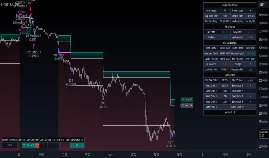
🟣 Trade Example
A clear example of a trade. Base order entry, safety order 1 fills, take profit 1 hits at 1%, the remainder of the position runs until the exit signal fires.
🟣 Warning
This tool has been developed to support your trading analysis, yet it’s important to acknowledge the inherent risks associated with trading. It is advisable to perform thorough research, assess your risk tolerance, and utilise this tool as one element of an overall trading strategy. Ensure that you only trade with capital that you are prepared to risk. In addition, due to the complexity of the tool, bugs may be found. Please alert us whenever you think you have found a bug in the system.
Multi-TF AI SuperTrend with ADX - Strategy [PresentTrading]
## █ Introduction and How it is Different
The trading strategy in question is an enhanced version of the SuperTrend indicator, combined with AI elements and an ADX filter. It's a multi-timeframe strategy that incorporates two SuperTrends from different timeframes and utilizes a k-nearest neighbors (KNN) algorithm for trend prediction. It's different from traditional SuperTrend indicators because of its AI-based predictive capabilities and the addition of the ADX filter for trend strength.
BTC 8hr Performance
ETH 8hr Performance
## █ Strategy, How it Works: Detailed Explanation (Revised)
### Multi-Timeframe Approach
The strategy leverages the power of multiple timeframes by incorporating two SuperTrend indicators, each calculated on a different timeframe. This multi-timeframe approach provides a holistic view of the market's trend. For example, a 8-hour timeframe might capture the medium-term trend, while a daily timeframe could capture the longer-term trend. When both SuperTrends align, the strategy confirms a more robust trend.
### K-Nearest Neighbors (KNN)
The KNN algorithm is used to classify the direction of the trend based on historical SuperTrend values. It uses weighted voting of the 'k' nearest data points. For each point, it looks at its 'k' closest neighbors and takes a weighted average of their labels to predict the current label. The KNN algorithm is applied separately to each timeframe's SuperTrend data.
### SuperTrend Indicators
Two SuperTrend indicators are used, each from a different timeframe. They are calculated using different moving averages and ATR lengths as per user settings. The SuperTrend values are then smoothed to make them suitable for KNN-based prediction.
### ADX and DMI Filters
The ADX filter is used to eliminate weak trends. Only when the ADX is above 20 and the directional movement index (DMI) confirms the trend direction, does the strategy signal a buy or sell.
### Combining Elements
A trade signal is generated only when both SuperTrends and the ADX filter confirm the trend direction. This multi-timeframe, multi-indicator approach reduces false positives and increases the robustness of the strategy.
By considering multiple timeframes and using machine learning for trend classification, the strategy aims to provide more accurate and reliable trade signals.
BTC 8hr Performance (Zoom-in)
## █ Trade Direction
The strategy allows users to specify the trade direction as 'Long', 'Short', or 'Both'. This is useful for traders who have a specific market bias. For instance, in a bullish market, one might choose to only take 'Long' trades.
## █ Usage
Parameters: Adjust the number of neighbors, data points, and moving averages according to the asset and market conditions.
Trade Direction: Choose your preferred trading direction based on your market outlook.
ADX Filter: Optionally, enable the ADX filter to avoid trading in a sideways market.
Risk Management: Use the trailing stop-loss feature to manage risks.
## █ Default Settings
Neighbors (K): 3
Data points for KNN: 12
SuperTrend Length: 10 and 5 for the two different SuperTrends
ATR Multiplier: 3.0 for both
ADX Length: 21
ADX Time Frame: 240
Default trading direction: Both
By customizing these settings, traders can tailor the strategy to fit various trading styles and assets.
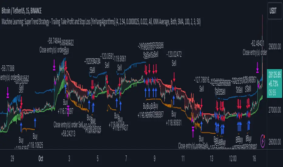
Machine Learning: SuperTrend Strategy TP/SL [YinYangAlgorithms]The SuperTrend is a very useful Indicator to display when trends have shifted based on the Average True Range (ATR). Its underlying ideology is to calculate the ATR using a fixed length and then multiply it by a factor to calculate the SuperTrend +/-. When the close crosses the SuperTrend it changes direction.
This Strategy features the Traditional SuperTrend Calculations with Machine Learning (ML) and Take Profit / Stop Loss applied to it. Using ML on the SuperTrend allows for the ability to sort data from previous SuperTrend calculations. We can filter the data so only previous SuperTrends that follow the same direction and are within the distance bounds of our k-Nearest Neighbour (KNN) will be added and then averaged. This average can either be achieved using a Mean or with an Exponential calculation which puts added weight on the initial source. Take Profits and Stop Losses are then added to the ML SuperTrend so it may capitalize on Momentum changes meanwhile remaining in the Trend during consolidation.
By applying Machine Learning logic and adding a Take Profit and Stop Loss to the Traditional SuperTrend, we may enhance its underlying calculations with potential to withhold the trend better. The main purpose of this Strategy is to minimize losses and false trend changes while maximizing gains. This may be achieved by quick reversals of trends where strategic small losses are taken before a large trend occurs with hopes of potentially occurring large gain. Due to this logic, the Win/Loss ratio of this Strategy may be quite poor as it may take many small marginal losses where there is consolidation. However, it may also take large gains and capitalize on strong momentum movements.
Tutorial:
In this example above, we can get an idea of what the default settings may achieve when there is momentum. It focuses on attempting to hit the Trailing Take Profit which moves in accord with the SuperTrend just with a multiplier added. When momentum occurs it helps push the SuperTrend within it, which on its own may act as a smaller Trailing Take Profit of its own accord.
We’ve highlighted some key points from the last example to better emphasize how it works. As you can see, the White Circle is where profit was taken from the ML SuperTrend simply from it attempting to switch to a Bullish (Buy) Trend. However, that was rejected almost immediately and we went back to our Bearish (Sell) Trend that ended up resulting in our Take Profit being hit (Yellow Circle). This Strategy aims to not only capitalize on the small profits from SuperTrend to SuperTrend but to also capitalize when the Momentum is so strong that the price moves X% away from the SuperTrend and is able to hit the Take Profit location. This Take Profit addition to this Strategy is crucial as momentum may change state shortly after such drastic price movements; and if we were to simply wait for it to come back to the SuperTrend, we may lose out on lots of potential profit.
If you refer to the Yellow Circle in this example, you’ll notice what was talked about in the Summary/Overview above. During periods of consolidation when there is little momentum and price movement and we don’t have any Stop Loss activated, you may see ‘Signal Flashing’. Signal Flashing is when there are Buy and Sell signals that keep switching back and forth. During this time you may be taking small losses. This is a normal part of this Strategy. When a signal has finally been confirmed by Momentum, is when this Strategy shines and may produce the profit you desire.
You may be wondering, what causes these jagged like patterns in the SuperTrend? It's due to the ML logic, and it may be a little confusing, but essentially what is happening is the Fast Moving SuperTrend and the Slow Moving SuperTrend are creating KNN Min and Max distances that are extreme due to (usually) parabolic movement. This causes fewer values to be added to and averaged within the ML and causes less smooth and more exponential drastic movements. This is completely normal, and one of the perks of using k-Nearest Neighbor for ML calculations. If you don’t know, the Min and Max Distance allowed is derived from the most recent(0 index of data array) to KNN Length. So only SuperTrend values that exhibit distances within these Min/Max will be allowed into the average.
Since the KNN ML logic can cause these exponential movements in the SuperTrend, they likewise affect its Take Profit. The Take Profit may benefit from this movement like displayed in the example above which helped it claim profit before then exhibiting upwards movement.
By default our Stop Loss Multiplier is kept quite low at 0.0000025. Keeping it low may help to reduce some Signal Flashing while not taking extra losses more so than not using it at all. However, if we increase it even more to say 0.005 like is shown in the example above. It can really help the trend keep momentum. Please note, although previous results don’t imply future results, at 0.0000025 Stop Loss we are currently exhibiting 69.27% profit while at 0.005 Stop Loss we are exhibiting 33.54% profit. This just goes to show that although there may be less Signal Flashing, it may not result in more profit.
We will conclude our Tutorial here. Hopefully this has given you some insight as to how Machine Learning, combined with Trailing Take Profit and Stop Loss may have positive effects on the SuperTrend when turned into a Strategy.
Settings:
SuperTrend:
ATR Length: ATR Length used to create the Original Supertrend.
Factor: Multiplier used to create the Original Supertrend.
Stop Loss Multiplier: 0 = Don't use Stop Loss. Stop loss can be useful for helping to prevent false signals but also may result in more loss when hit and less profit when switching trends.
Take Profit Multiplier: Take Profits can be useful within the Supertrend Strategy to stop the price reverting all the way to the Stop Loss once it's been profitable.
Machine Learning:
Only Factor Same Trend Direction: Very useful for ensuring that data used in KNN is not manipulated by different SuperTrend Directional data. Please note, it doesn't affect KNN Exponential.
Rationalized Source Type: Should we Rationalize only a specific source, All or None?
Machine Learning Type: Are we using a Simple ML Average, KNN Mean Average, KNN Exponential Average or None?
Machine Learning Smoothing Type: How should we smooth our Fast and Slow ML Datas to be used in our KNN Distance calculation? SMA, EMA or VWMA?
KNN Distance Type: We need to check if distance is within the KNN Min/Max distance, which distance checks are we using.
Machine Learning Length: How far back is our Machine Learning going to keep data for.
k-Nearest Neighbour (KNN) Length: How many k-Nearest Neighbours will we account for?
Fast ML Data Length: What is our Fast ML Length?? This is used with our Slow Length to create our KNN Distance.
Slow ML Data Length: What is our Slow ML Length?? This is used with our Fast Length to create our KNN Distance.
If you have any questions, comments, ideas or concerns please don't hesitate to contact us.
HAPPY TRADING!
Machine Learning: Donchian DCA Grid Strategy [YinYangAlgorithms]This strategy uses a Machine Learning approach on the Donchian Channels with a DCA and Grid purchase/sell Strategy. Not only that, but it uses a custom Bollinger calculation to determine its Basis which is used as a mild sell location. This strategy is a pure DCA strategy in the sense that no shorts are used and theoretically it can be used in webhooks on most exchanges as it’s only using Spot Orders. The idea behind this strategy is we utilize both the Highest Highs and Lowest Lows within a Machine Learning standpoint to create Buy and Sell zones. We then fraction these zones off into pieces to create Grids. This allows us to ‘micro’ purchase as it enters these zones and likewise ‘micro’ sell as it goes up into the upper (sell) zones.
You have the option to set how many grids are used, by default we use 100 with max 1000. These grids can be ‘stacked’ together if a single bar is to go through multiple at the same time. For instance, if a bar goes through 30 grids in one bar, it will have a buy/sell power of 30x. Stacking Grid Buy and (sometimes) Sells is a very crucial part of this strategy that allows it to purchase multitudes during crashes and capitalize on sales during massive pumps.
With the grids, you’ll notice there is a middle line within the upper and lower part that makes the grid. As a Purchase Type within our Settings this is identified as ‘Middle of Zone Purchase Amount In USDT’. The middle of the grid may act as the strongest grid location (aside from maybe the bottom). Therefore there is a specific purchase amount for this Grid location.
This DCA Strategy also features two other purchase methods. Most importantly is its ‘Purchase More’ type. Essentially it will attempt to purchase when the Highest High or Lowest Low moves outside of the Outer band. For instance, the Lowest Low becomes Lower or the Higher High becomes Higher. When this happens may be a good time to buy as it is featuring a new High or Low over an extended period.
The last but not least Purchase type within this Strategy is what we call a ‘Strong Buy’. The reason for this is its verified by the following:
The outer bounds have been pushed (what causes a ‘Purchase More’)
The Price has crossed over the EMA 21
It has been verified through MACD, RSI or MACD Historical (Delta) using Regular and Hidden Divergence (Note, only 1 of these verifications is required and it can be any).
By default we don’t have Purchase Amount for ‘Strong Buy’ set, but that doesn’t mean it can’t be viable, it simply means we have only seen a few pairs where it actually proved more profitable allocating money there rather than just increasing the purchase amount for ‘Purchase More’ or ‘Grids’.
Now that you understand where we BUY, we should discuss when we SELL.
This Strategy features 3 crucial sell locations, and we will discuss each individually as they are very important.
1. ‘Sell Some At’: Here there are 4 different options, by default its set to ‘Both’ but you can change it around if you want. Your options are:
‘Both’ - You will sell some at both locations. The amount sold is the % used at ‘Sell Some %’.
‘Basis Line’ - You will sell some when the price crosses over the Basis Line. The amount sold is the % used at ‘Sell Some %’.
‘Percent’ - You will sell some when the Close is >= X% between the Lower Inner and Upper Inner Zone.
‘None’ - This simply means don’t ever Sell Some.
2. Sell Grids. Sell Grids are exactly like purchase grids and feature the same amount of grids. You also have the ability to ‘Stack Grid Sells’, which basically means if a bar moves multiple grids, it will stack the amount % wise you will sell, rather than just selling the default amount. Sell Grids use a DCA logic but for selling, which we deem may help adjust risk/reward ratio for selling, especially if there is slow but consistent bullish movement. It causes these grids to constantly push up and therefore when the close is greater than them, accrue more profit.
3. Take Profit. Take profit occurs when the close first goes above the Take Profit location (Teal Line) and then Closes below it. When Take Profit occurs, ALL POSITIONS WILL BE SOLD. What may happen is the price enters the Sell Grid, doesn’t go all the way to the top ‘Exiting it’ and then crashes back down and closes below the Take Profit. Take Profit is a strong location which generally represents a strong profit location, and that a strong momentum has changed which may cause the price to revert back to the buy grid zone.
Keep in mind, if you have (by default) ‘Only Sell If Profit’ toggled, all sell locations will only create sell orders when it is profitable to do so. Just cause it may be a good time to sell, doesn’t mean based on your DCA it is. In our opinion, only selling when it is profitable to do so is a key part of the DCA purchase strategy.
You likewise have the ability to ‘Only Buy If Lower than DCA’, which is likewise by default. These two help keep the Yin and Yang by balancing each other out where you’re only purchasing and selling when it makes logical sense too, even if that involves ignoring a signal and waiting for a better opportunity.
Tutorial:
Like most of our Strategies, we try to capitalize on lower Time Frames, generally the 15 minutes so we may find optimal entry and exit locations while still maintaining a strong correlation to trend patterns.
First off, let’s discuss examples of how this Strategy works prior to applying Machine Learning (enabled by default).
In this example above we have disabled the showing of ‘Potential Buy and Sell Signals’ so as to declutter the example. In here you can see where actual trades had gone through for both buying and selling and get an idea of how the strategy works. We also have disabled Machine Learning for this example so you can see the hard lines created by the Donchian Channel. You can also see how the Basis line ‘white line’ may act as a good location to ‘Sell Some’ and that it moves quite irregularly compared to the Donchian Channel. This is due to the fact that it is based on two custom Bollinger Bands to create the basis line.
Here we zoomed out even further and moved back a bit to where there were dense clusters of buy and sell orders. Sometimes when the price is rather volatile you’ll see it ‘Ping Pong’ back and forth between the buy and sell zones quite quickly. This may be very good for your trades and profit as a whole, especially if ‘Only Buy If Lower Than DCA’ and ‘Only Sell If Profit’ are both enabled; as these toggles will ensure you are:
Always lowering your Average when buying
Always making profit when selling
By default 8% commission is added to the Strategy as well, to simulate the cost effects of if these trades were taking place on an actual exchange.
In this example we also turned on the visuals for our ‘Purchase More’ (orange line) and ‘Take Profit’ (teal line) locations. These are crucial locations. The Purchase More makes purchases when the bottom of the grid has been moved (may dictate strong price movement has occurred and may be potential for correction). Our Take Profit may help secure profit when a momentum change is happening and all of the Sell Grids weren’t able to be used.
In the example above we’ve enabled Buy and Sell Signals so that you can see where the Take Profit and Purchase More signals have occurred. The white circle demonstrates that not all of the Position Size was sold within the Sell Grids, and therefore it was ALL CLOSED when the price closed below the Take Profit Line (Teal).
Then, when the bottom of the Donchian Channel was pushed further down due to the close (within the yellow circle), a Purchase More Signal was triggered.
When the close keeps pushing the bottom of the Buy Grid lower, it can cause multiple Purchase More Signals to occur. This is normal and also a crucial part of this strategy to help lower your DCA. Please note, the Purchase More won’t trigger a Buy if the Close is greater than the DCA and you have ‘Only Purchase If Lower Than DCA’ activated.
By turning on Machine Learning (default settings) the Buy and Sell Grid Zones are smoothed out more. It may cause it to look quite a bit different. Machine Learning although it looks much worse, may help increase the profit this Strategy can produce. Previous results DO NOT mean future results, but in this example, prior to turning on Machine Learning it had produced 37% Profit in ~5 months and with Machine Learning activated it is now up to 57% Profit in ~5 months.
Machine Learning causes the Strategy to focus less on Grids and more on Purchase More when it comes to getting its entries. However, if you likewise attempt to focus on Purchase More within non Machine Learning, the locations are different and therefore the results may not be as profitable.
PLEASE NOTE:
By default this strategy uses 1,000,000 as its initial capital. The amount it purchases in its Settings is relevant to this Initial capital. Considering this is a DCA Strategy, we only want to ‘Micro’ Buy and ‘Micro’ Sell whenever conditions are met.
Therefore, if you increase the Initial Capital, you’ll likewise want to increase the Purchase Amounts within the Settings and Vice Versa. For instance, if you wish to set the Initial Capital to 10,000, you should likewise can the amounts in the Settings to 1% of what they are to account for this.
We may change the Purchase Amounts to be based on %’s in a later update if it is requested.
We will conclude this Tutorial here, hopefully you can see how a DCA Grid Purchase Model applied to Machine Learning Donchian Channels may be useful for making strategic purchases in low and high zones.
Settings:
Display Data:
Show Potential Buy Locations: These locations are where 'Potentially' orders can be placed. Placement of orders is dependant on if you have 'Only Buy If Lower Than DCA' toggled and the Price is lower than DCA. It also is effected by if you actually have any money left to purchase with; you can't buy if you have no money left!
Show Potential Sell Locations: These locations are where 'Potentially' orders will be sold. If 'Only Sell If Profit' is toggled, the sell will only happen if you'll make profit from it!
Show Grid Locations: Displaying won't affect your trades but it can be useful to see where trades will be placed, as well as which have gone through and which are left to be purchased. Max 100 Grids, but visuals will only be shown if its 20 or less.
Purchase Settings:
Only Buy if its lower than DCA: Generally speaking, we want to lower our Average, and therefore it makes sense to only buy when the close is lower than our current DCA and a Purchase Condition is met.
Compound Purchases: Compounding Purchases means reinvesting profit back into your trades right away. It drastically increases profits, but it also increases risk too. It will adjust your Purchase Amounts for the Purchase Type you have set at the same % rate of strategy initial_capital to the amounts you have set.
Adjust Purchase Amount Ratio to Maintain Risk level: By adjusting purchase levels we generally help maintain a safe risk level. Basically we generally want to reserve X amount of % for each purchase type being used and relocate money when there is too much in one type. This helps balance out purchase amounts and ensure the types selected have a correct ratio to ensure they can place the right amount of orders.
Stack Grid Buys: Stacking Buy Grids is when the Close crosses multiple Buy Grids within the same bar. Should we still only purchase the value of 1 Buy Grid OR stack the grid buys based on how many buy grids it went through.
Purchase Type: Where do you want to make Purchases? We recommend lowering your risk by combining All purchase types, but you may also customize your trading strategy however you wish.
Strong Buy Purchase Amount In USDT: How much do you want to purchase when the 'Strong Buy' signal appears? This signal only occurs after it has at least entered the Buy Zone and there have been other verifications saying it's now a good time to buy. Our Strong Buy Signal is a very strong indicator that a large price movement towards the Sell Zone will likely occur. It almost always results in it leaving the Buy Zone and usually will go to at least the White Basis line where you can 'Sell Some'.
Buy More Purchase Amount In USDT: How much should you purchase when the 'Purchase More' signal appears? This 'Purchase More' signal occurs when the lowest level of the Buy Zone moves lower. This is a great time to buy as you're buying the dip and generally there is a correction that will allow you to 'Sell Some' for some profit.
Amount of Grid Buy and Sells: How many Grid Purchases do you want to make? We recommend having it at the max of 10, as it will essentially get you a better Average Purchase Price, but you may adjust it to whatever you wish. This amount also only matters if your Purchase Type above incorporates Grid Purchases. Max 100 Grids, but visuals will only be shown if it's 20 or less.
Each Grid Purchase Amount In USDT: How much should you purchase after closing under a grid location? Keep in mind, if you have 10 grids and it goes through each, it will be this amount * 10. Grid purchasing is a great way to get a good entry, lower risk and also lower your average.
Middle Of Zone Purchase Amount In USDT: The Middle Of Zone is the strongest grid location within the Buy Zone. This is why we have a unique Purchase Amount for this Grid specifically. Please note you need to have 'Middle of Zone is a Grid' enabled for this Purchase Amount to be used.
Sell:
Only Sell if its Profit: There is a chance that during a dump, all your grid buys when through, and a few Purchase More Signals have appeared. You likely got a good entry. A Strong Buy may also appear before it starts to pump to the Sell Zone. The issue that may occur is your Average Purchase Price is greater than the 'Sell Some' price and/or the Grids in the Sell Zone and/or the Strong Sell Signal. When this happens, you can either take a loss and sell it, or you can hold on to it and wait for more purchase signals to therefore lower your average more so you can take profit at the next sell location. Please backtest this yourself within our YinYang Purchase Strategy on the pair and timeframe you are wanting to trade on. Please also note, that previous results will not always reflect future results. Please assess the risk yourself. Don't trade what you can't afford to lose. Sometimes it is better to strategically take a loss and continue on making profit than to stay in a bad trade for a long period of time.
Stack Grid Sells: Stacking Sell Grids is when the Close crosses multiple Sell Grids within the same bar. Should we still only sell the value of 1 Sell Grid OR stack the grid sells based on how many sell grids it went through.
Stop Loss Type: This is when the Close has pushed the Bottom of the Buy Grid More. Do we Stop Loss or Purchase More?? By default we recommend you stay true to the DCA part of this strategy by Purchasing More, but this is up to you.
Sell Some At: Where if selected should we 'Sell Some', this may be an important way to sell a little bit at a good time before the price may correct. Also, we don't want to sell too much incase it doesn't correct though, so its a 'Sell Some' location. Basis Line refers to our Moving Basis Line created from 2 Bollinger Bands and Percent refers to a Percent difference between the Lower Inner and Upper Inner bands.
Sell Some At Percent Amount: This refers to how much % between the Lower Inner and Upper Inner bands we should well at if we chose to 'Sell Some'.
Sell Some Min %: This refers to the Minimum amount between the Lower Inner band and Close that qualifies a 'Sell Some'. This acts as a failsafe so we don't 'Sell Some' for too little.
Sell % At Strong Sell Signal: How much do we sell at the 'Strong Sell' Signal? It may act as a strong location to sell, but likewise Grid Sells could be better.
Grid and Donchian Settings:
Donchian Channel Length: How far back are we looking back to determine our Donchian Channel.
Extra Outer Buy Width %: How much extra should we push the Outer Buy (Low) Width by?
Extra Inner Buy Width %: How much extra should we push the Inner Buy (Low) Width by?
Extra Inner Sell Width %: How much extra should we push the Inner Sell (High) Width by?
Extra Outer Sell Width %: How much extra should we push the Outer Sell (High) Width by?
Machine Learning:
Rationalized Source Type: Donchians usually use High/Low. What Source is our Rationalized Source using?
Machine Learning Type: Are we using a Simple ML Average, KNN Mean Average, KNN Exponential Average or None?
Machine Learning Length: How far back is our Machine Learning going to keep data for.
k-Nearest Neighbour (KNN) Length: How many k-Nearest Neighbours will we account for?
Fast ML Data Length: What is our Fast ML Length?? This is used with our Slow Length to create our KNN Distance.
Slow ML Data Length: What is our Slow ML Length?? This is used with our Fast Length to create our KNN Distance.
If you have any questions, comments, ideas or concerns please don't hesitate to contact us.
HAPPY TRADING!
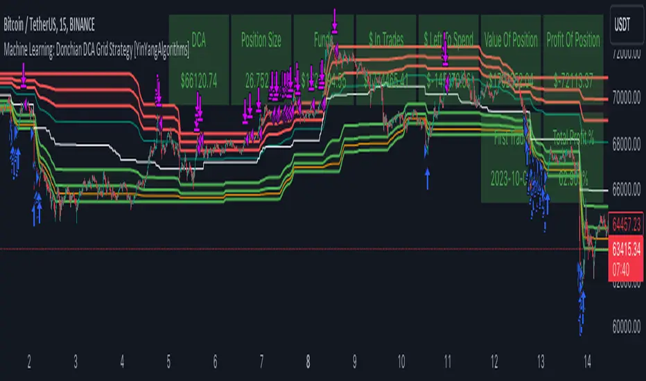
Double AI Super Trend Trading - Strategy [PresentTrading]█ Introduction and How It is Different
The Double AI Super Trend Trading Strategy is a cutting-edge approach that leverages the power of not one, but two AI algorithms, in tandem with the SuperTrend technical indicator. The strategy aims to provide traders with enhanced precision in market entry and exit points. It is designed to adapt to market conditions dynamically, offering the flexibility to trade in both bullish and bearish markets.
*The KNN part is mainly referred from @Zeiierman.
BTCUSD 8hr performance
ETHUSD 8hr performance
█ Strategy, How It Works: Detailed Explanation
1. SuperTrend Calculation
The SuperTrend is a popular indicator that captures market trends through a combination of the Volume-Weighted Moving Average (VWMA) and the Average True Range (ATR). This strategy utilizes two sets of SuperTrend calculations with varying lengths and factors to capture both short-term and long-term market trends.
2. KNN Algorithm
The strategy employs k-Nearest Neighbors (KNN) algorithms, which are supervised machine learning models. Two sets of KNN algorithms are used, each focused on different lengths of historical data and number of neighbors. The KNN algorithms classify the current SuperTrend data point as bullish or bearish based on the weighted sum of the labels of the k closest historical data points.
3. Signal Generation
Based on the KNN classifications and the SuperTrend indicator, the strategy generates signals for the start of a new trend and the continuation of an existing trend.
4. Trading Logic
The strategy uses these signals to enter long or short positions. It also incorporates dynamic trailing stops for exit conditions.
Local picture
█ Trade Direction
The strategy allows traders to specify their trading direction: long, short, or both. This enables the strategy to be versatile and adapt to various market conditions.
█ Usage
ToolTips: Comprehensive tooltips are provided for each parameter to guide the user through the customization process.
Inputs: Traders can customize numerous parameters including the number of neighbors in KNN, ATR multiplier, and types of moving averages.
Plotting: The strategy also provides visual cues on the chart to indicate bullish or bearish trends.
Order Execution: Based on the generated signals, the strategy will execute buy or sell orders automatically.
█ Default Settings
The default settings are configured to offer a balanced approach suitable for most scenarios:
Initial Capital: $10,000
Default Quantity Type: 10% of equity
Commission: 0.1%
Slippage: 1
Currency: USD
These settings can be modified to suit various trading styles and asset classes.
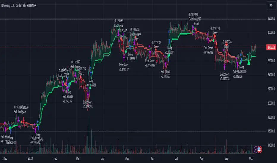
IU Break of any session StrategyHow this script works:
1. This script is an intraday trading strategy script which buy and sell on the bases of user-defined intraday session range breakout and gives alert(if the alert is set) message too when the new position is open.
2. It calculate the session as per the user inputs or user defined custom session.
3. The script stores the highest and lowest value of the whole session.
4. It take a long position on the first break and close above the highest value.
5. It take a short position on the break and close below the lowest value.
6. The script takes one position in one day.
7. The stop loss for this script is the previous low(if long) or high(if short).
8. Take profit is 1:2 and it's adjustable.
9. This script work on every kind of market.
How The Useful For The User :
1. User can backtest any session range breakout he wants to trade.
2. User can get alert when the new position is open.
3. User can change the Risk to Reward in order to find the best Risk to Reward.
4. User can see the highest and lowest value of the session with respect to analyzing his trading objective.
5. This strategy script highlights which session range breakout performs best and which performs worst.

AI SuperTrend - Strategy [presentTrading]
█ Introduction and How it is Different
The AI Supertrend Strategy is a unique hybrid approach that employs both traditional technical indicators and machine learning techniques. Unlike standard strategies that rely solely on traditional indicators or mathematical models, this strategy integrates the power of k-Nearest Neighbors (KNN), a machine learning algorithm, with the tried-and-true SuperTrend indicator. This blend aims to provide traders with more accurate, responsive, and context-aware trading signals.
*The KNN part is mainly referred from @Zeiierman.
BTCUSD 8hr performance
ETHUSD 8hr performance
█ Strategy, How it Works: Detailed Explanation
SuperTrend Calculation
Volume-Weighted Moving Average (VWMA): A VWMA of the close price is calculated based on the user-defined length (len). This serves as the central line around which the upper and lower bands are calculated.
Average True Range (ATR): ATR is calculated over a period defined by len. It measures the market's volatility.
Upper and Lower Bands: The upper band is calculated as VWMA + (factor * ATR) and the lower band as VWMA - (factor * ATR). The factor is a user-defined multiplier that decides how wide the bands should be.
KNN Algorithm
Data Collection: An array (data) is populated with recent n SuperTrend values. Corresponding labels (labels) are determined by whether the weighted moving average price (price) is greater than the weighted moving average of the SuperTrend (sT).
Distance Calculation: The absolute distance between each data point and the current SuperTrend value is calculated.
Sorting & Weighting: The distances are sorted in ascending order, and the closest k points are selected. Each point is weighted by the inverse of its distance to the current point.
Classification: A weighted sum of the labels of the k closest points is calculated. If the sum is closer to 1, the trend is predicted as bullish; if closer to 0, bearish.
Signal Generation
Start of Trend: A new bullish trend (Start_TrendUp) is considered to have started if the current trend color is bullish and the previous was not bullish. Similarly for bearish trends (Start_TrendDn).
Trend Continuation: A bullish trend (TrendUp) is considered to be continuing if the direction is negative and the KNN prediction is 1. Similarly for bearish trends (TrendDn).
Trading Logic
Long Condition: If Start_TrendUp or TrendUp is true, a long position is entered.
Short Condition: If Start_TrendDn or TrendDn is true, a short position is entered.
Exit Condition: Dynamic trailing stops are used for exits. If the trend does not continue as indicated by the KNN prediction and SuperTrend direction, an exit signal is generated.
The synergy between SuperTrend and KNN aims to filter out noise and produce more reliable trading signals. While SuperTrend provides a broad sense of the market direction, KNN refines this by predicting short-term price movements, leading to a more nuanced trading strategy.
Local picture
█ Trade Direction
The strategy allows traders to choose between taking only long positions, only short positions, or both. This is particularly useful for adapting to different market conditions.
█ Usage
ToolTips: Explains what each parameter does and how to adjust them.
Inputs: Customize values like the number of neighbors in KNN, ATR multiplier, and moving average type.
Plotting: Visual cues on the chart to indicate bullish or bearish trends.
Order Execution: Based on the generated signals, the strategy will execute buy/sell orders.
█ Default Settings
The default settings are selected to provide a balanced approach, but they can be modified for different trading styles and asset classes.
Initial Capital: $10,000
Default Quantity Type: 10% of equity
Commission: 0.1%
Slippage: 1
Currency: USD
By combining both machine learning and traditional technical analysis, this strategy offers a sophisticated and adaptive trading solution.
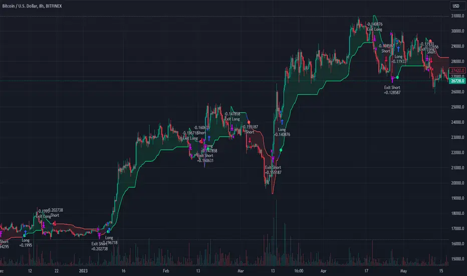
Hoffman Heiken BiasThis indicator uses a couple of different things including the Hoffman moving averages applied with heiken ashi bar data and some volatility to help determine when the bias of the market has shifted for the timeframe you are looking at.
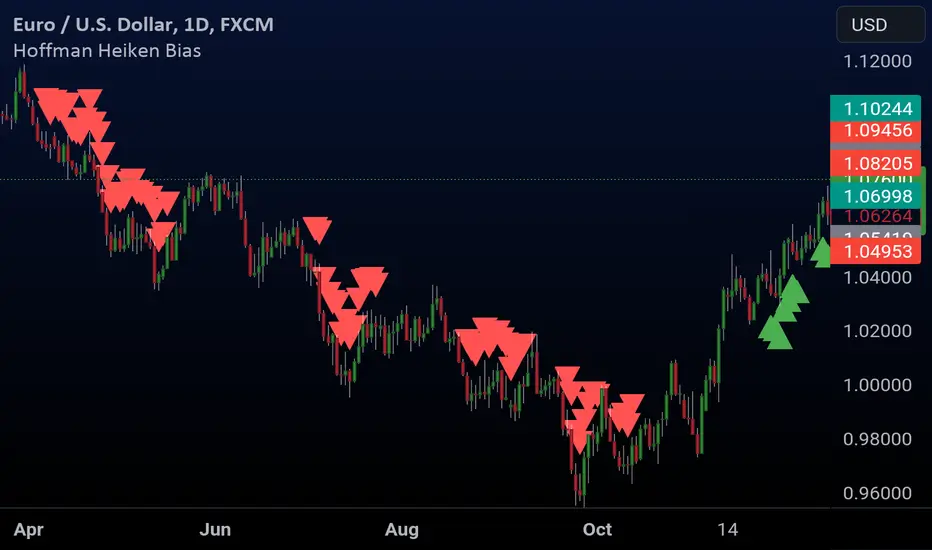
Gaussian Detrended ReversionThis strategy, titled "Gaussian Detrended Reversion Strategy," aims to identify potential price reversals using the customized Gaussian Detrended Price Oscillator (GDPO) in combination with smoothed price cycles.
Key Elements of the Strategy:
GDPO Calculation: The strategy first calculates the Detrended Price Oscillator (DPO) by comparing the close price to an Exponential Moving Average (EMA) of a specified period. This calculation helps identify short-term price cycles by detrending the price data.
Gaussian Smoothing: The DPO values are then smoothed using the Arnaud Legoux Moving Average (ALMA), applying a Gaussian smoothing technique. This smoothed version of the DPO is intended to filter out noise and provide a clearer picture of price trends.
Entry and Exit Conditions: The strategy defines conditions for both long and short entry points as well as exit points. It looks for specific crossover events between the smoothed GDPO and its lagged version. The strategy enters a long position when the smoothed GDPO crosses above the lag and is negative, and exits the long position when the smoothed GDPO crosses below the lag or the zero line. Similarly, the strategy enters a short position when the smoothed GDPO crosses below the lag and is positive, and exits the short position when the smoothed GDPO crosses above the lag or the zero line.
Visualization: The smoothed GDPO and its lag are plotted on the chart using distinct colors. The zero line is also displayed as a reference point. Additionally, the chart background changes color when the strategy enters a long or short position. Cross markers are also plotted at the crossover points as exit cues.
Overall, this strategy aims to capture potential price reversals using the GDPO and Gaussian smoothing, with specific entry and exit conditions to guide trading decisions.
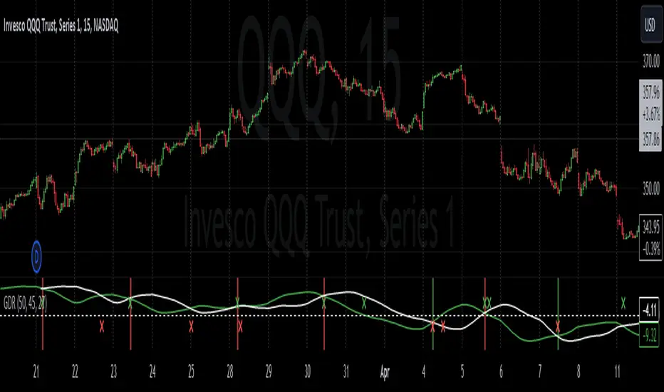
Nadaraya-Watson Envelope Strategy (Non-Repainting) Log ScaleIn the diverse world of trading strategies, the Nadaraya-Watson Envelope Strategy offers a different approach. Grounded in mathematical analysis, this strategy utilizes the Nadaraya-Watson kernel regression, a method traditionally employed for interpreting complex data patterns.
At the core of this strategy lies the concept of 'envelopes', which are essentially dynamic volatility bands formed around the price based on a custom Average True Range (ATR). These envelopes help provide guidance on potential market entry and exit points. The strategy suggests considering a buy when the price crosses the lower envelope and a sell when it crosses the upper envelope.
One distinctive characteristic of the Nadaraya-Watson Envelope Strategy is its use of a logarithmic scale, as opposed to a linear scale. The logarithmic scale can be advantageous when dealing with larger timeframes and assets with wide-ranging price movements.
The strategy is implemented using Pine Script v5, and includes several adjustable parameters such as the lookback window, relative weighting, and the regression start point, providing a level of flexibility.
However, it's important to maintain a balanced view. While the use of mathematical models like the Nadaraya-Watson kernel regression may provide insightful data analysis, no strategy can guarantee success. Thorough backtesting, understanding the mathematical principles involved, and sound risk management are always essential when applying any trading strategy.
The Nadaraya-Watson Envelope Strategy thus offers another tool for traders to consider. As with all strategies, its effectiveness will largely depend on the trader's understanding, application, and the specific market conditions.
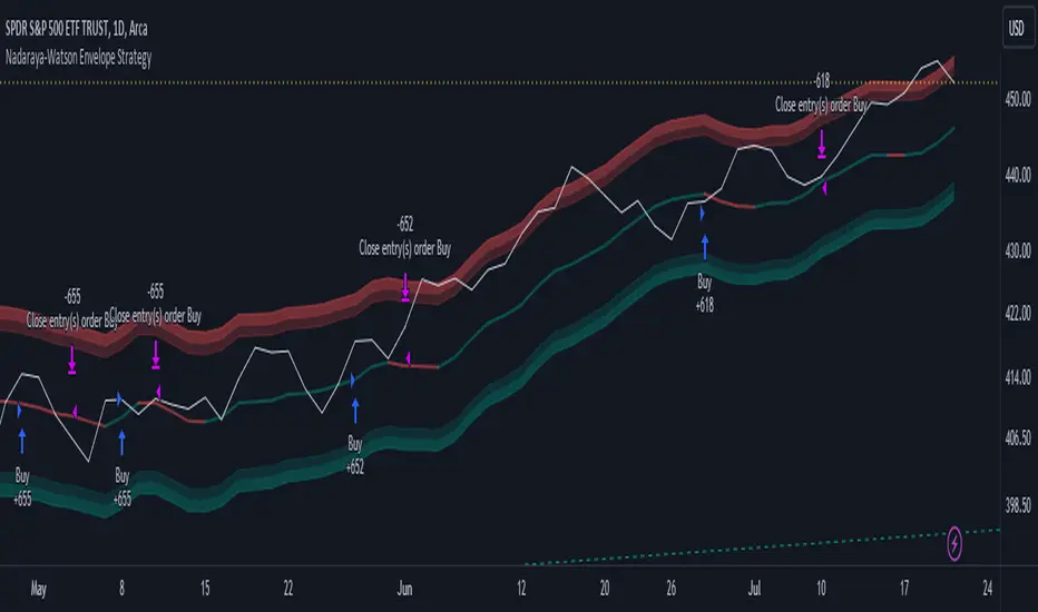
Crunchster's Normalised Trend StrategyThis is a unique rules-based, systematic trading strategy - in the trend following category.
The strategy is designed for use on the daily timeframe. Specific features of this strategy are outlined below:
1. Uses a transformed price series (which I dub "real price") to generate signals rather than ticker price
2. Uses advanced position sizing and risk management, usually reserved for institutional portfolio management, a proven technique utilised by Commodity Trading Advisors and Managed Futures funds (Algo/Quant funds).
"Real Price" is a transformed price series derived from the sum of volatility adjusted (daily) returns, over the entire price series of an asset. The lookback period of the volatility adjustment is user defined.
A Hull moving average (HMA) is derived from the real price, and used as the main trend determinant. The lookback period of the HMA is user defined. Default lookback of 100 periods (days) ensures a responsive trend indicator, but without leading to over-trading from frequent crossovers (average holding period 14 days on BTC).
The core strategy is very simple, go long when real price crosses over HMA, go short when real price crosses under HMA. New position triggers automatically close open positions in the counter direction.
Position sizing is based on recent price volatility and the user defined annualised risk target. In essence positions are inverse volatility weighted, so larger size is opened during lower volatility and smaller size during increased volatility. Recent volatility is calculated as the standard deviation of returns with 14 period lookback, then extrapolated into an annualised volatility of expected returns. Annualised recent volatility is then referenced to the risk target set by the user to adjust the position size. The default settings are a very conservative 10% annual risk target. Initial capital should be set as the maximum risk capital per trade (ie if $10,000 total capital and 10% risk per trade, initial capital should be $1000). Maximum leverage per position can be set independently, to facilitate hitting risk targets that are greater than the natural volatility of the traded asset, and to accommodate low volatility conditions, whilst maintaining overall risk controls.
Hard stop losses are based on multiples of the average true range of recent price (14 period lookback), user configurable.
Please leave comments regarding further features or refinements. I plan to develop further adding alternative moving average selections and the ability to select/deselect long and short strategies.
3 hours ago
Release Notes:
Added option to compound profits versus using a fixed position capital. Be mindful that compounding will potentially increase profits, but also increase drawdowns and overall risk. Leverage will still cap overall exposure with compounding and therefore provides an additional layer of risk control.
2 hours ago
Release Notes:
Added function to toggle long/short strategy legs on and off.

SuperTrend Long Strategy +TrendFilterThis strategy aims to identify long (buy) opportunities in the market using the SuperTrend indicator. It utilizes the Average True Range (ATR) and a multiplier to determine the dynamic support levels for entering long positions. This presentation will provide an overview of the strategy's components, explain its usage, and highlight that it focuses on long trades.
Components of the Strategy:
1. ATR Period: This input determines the period used for calculating the Average True Range (ATR). A higher value may result in smoother trend lines but may lag behind recent price changes.
2. Source (src): This input determines the price source used for calculations, with "hl2" (the average of high and low prices) set as the default.
3. ATR Multiplier: This input specifies the multiplier applied to the ATR value to determine the distance of the support levels from the source.
4. Change ATR Calculation Method: This input allows toggling between two methods of ATR calculation: the default method using atr() or a simple moving average (SMA) of ATR values (sma(tr, Periods)).
5. Show Buy/Sell Signals: This input enables or disables the display of buy and sell signals on the chart.
6. Highlighter On/Off: This input controls whether highlighting of up and down trends is displayed on the chart.
7. Bar Coloring On/Off: This input determines whether the bars on the chart are colored based on the trend direction.
8. The "SuperTrend Long STRATEGY" has been enhanced by incorporating a trend filter. A moving average is used as the filter to confirm the prevailing trend before executing trades. This addition effectively reduces false signals and improves the strategy's reliability, all while maintaining its original name.
Strategy Logic:
1. The strategy calculates the upper (up) and lower (dn) trend lines based on the ATR value and the chosen multiplier.
2. The trend variable keeps track of the current trend, with 1 indicating an uptrend and -1 indicating a downtrend.
3. Buy and sell signals are generated based on the change in trend direction.
4. The strategy includes an optional highlighting feature that colors the chart background based on the current trend.
5. Additionally, the bar coloring feature colors the bars based on the direction of the last trend change.
Usage:
1. ATR Period and ATR Multiplier can be adjusted based on the desired sensitivity and risk tolerance.
2. Buy and sell signals can be displayed using the Show Buy/Sell Signals input, providing clear indications of entry and exit points.
3. The Highlighter On/Off input allows users to visually identify the prevailing trend by coloring the chart background.
4. The Bar Coloring On/Off input offers a quick visual reference for the most recent trend change.
Long Strategy:
The SuperTrend Long Strategy is specifically designed to identify long (buy) opportunities. It generates buy signals when the current trend changes from a downtrend to an uptrend, indicating a potential entry point for long positions. The strategy aims to capture upward price movements and maximize profits during bullish market conditions.
The SuperTrend Long Strategy provides traders with a systematic approach to identifying long trade opportunities. By leveraging the SuperTrend indicator and dynamic support levels, this strategy aims to generate buy signals in uptrending markets. Traders can customize the inputs and utilize the visual features to adapt the strategy to their specific trading preferences.
The modification adds a trend filter to the "SuperTrend Long STRATEGY" to improve its effectiveness. The trend filter uses a moving average to confirm the prevailing trend before taking trades. This addition helps filter out false signals and enhances the strategy's reliability without changing its name.

Lorentzian Classification Strategy Based in the model of Machine learning: Lorentzian Classification by @jdehorty, you will be able to get into trending moves and get interesting entries in the market with this strategy. I also put some new features for better backtesting results!
Backtesting context: 2022-07-19 to 2023-04-14 of US500 1H by PEPPERSTONE. Commissions: 0.03% for each entry, 0.03% for each exit. Risk per trade: 2.5% of the total account
For this strategy, 3 indicators are used:
Machine learning: Lorentzian Classification by @jdehorty
One Ema of 200 periods for identifying the trend
Supertrend indicator as a filter for some exits
Atr stop loss from Gatherio
Trade conditions:
For longs:
Close price is above 200 Ema
Lorentzian Classification indicates a buying signal
This gives us our long signal. Stop loss will be determined by atr stop loss (white point), break even(blue point) by a risk/reward ratio of 1:1 and take profit of 3:1 where half position will be closed. This will be showed as buy.
The other half will be closed when the model indicates a selling signal or Supertrend indicator gives a bearish signal. This will be showed as cl buy.
For shorts:
Close price is under 200 Ema
Lorentzian Classification indicates a selling signal
This gives us our short signal. Stop loss will be determined by atr stop loss (white point), break even(blue point) by a risk/reward ratio of 1:1 and take profit of 3:1 where half position will be closed. This will be showed as sell.
The other half will be closed when the model indicates a buying signal or Supertrend indicator gives a bullish signal. This will be showed as cl sell.
Risk management
To calculate the amount of the position you will use just a small percent of your initial capital for the strategy and you will use the atr stop loss or last swing for this.
Example: You have 1000 usd and you just want to risk 2,5% of your account, there is a buy signal at price of 4,000 usd. The stop loss price from atr stop loss or last swing is 3,900. You calculate the distance in percent between 4,000 and 3,900. In this case, that distance would be of 2.50%. Then, you calculate your position by this way: (initial or current capital * risk per trade of your account) / (stop loss distance).
Using these values on the formula: (1000*2,5%)/(2,5%) = 1000usd. It means, you have to use 1000 usd for risking 2.5% of your account.
We will use this risk management for applying compound interest.
> In settings, with position amount calculator, you can enter the amount in usd of your account and the amount in percentage for risking per trade of the account. You will see this value in green color in the upper left corner that shows the amount in usd to use for risking the specific percentage of your account.
> You can also choose a fixed amount, so you will have to activate fixed amount in risk management for trades and set the fixed amount for backtesting.
Script functions
Inside of settings, you will find some utilities for display atr stop loss, break evens, positions, signals, indicators, a table of some stats from backtesting, etc.
You will find the settings for risk management at the end of the script if you want to change something or trying new values for other assets for backtesting.
If you want to change the initial capital for backtest the strategy, go to properties, and also enter the commisions of your exchange and slippage for more realistic results.
In risk managment you can find an option called "Use leverage ?", activate this if you want to backtest using leverage, which means that in case of not having enough money for risking the % determined by you of your account using your initial capital, you will use leverage for using the enough amount for risking that % of your acount in a buy position. Otherwise, the amount will be limited by your initial/current capital
I also added a function for backtesting if you had added or withdrawn money frequently:
Adding money: You can choose how often you want to add money (Monthly, yearly, daily or weekly). Then a fixed amount of money and activate or deactivate this function
Withdraw money: You can choose if you want to withdraw a fixed amount or a percentage of earnings. Then you can choose a fixed amount of money, the period of time and activate or deactivate this function. Also, the percentage of earnings if you choosed this option.
Some other assets where strategy has worked
BTCUSD 4H, 1D
ETHUSD 4H, 1D
BNBUSD 4H
SPX 1D
BANKNIFTY 4H, 15 min
Some things to consider
USE UNDER YOUR OWN RISK. PAST RESULTS DO NOT REPRESENT THE FUTURE.
DEPENDING OF % ACCOUNT RISK PER TRADE, YOU COULD REQUIRE LEVERAGE FOR OPEN SOME POSITIONS, SO PLEASE, BE CAREFULL AND USE CORRECTLY THE RISK MANAGEMENT
Do not forget to change commissions and other parameters related with back testing results!. If you have problems loading the script reduce max bars back number in general settings
Strategies for trending markets use to have more looses than wins and it takes a long time to get profits, so do not forget to be patient and consistent !
Please, visit the post from @jdehorty called Machine Learning: Lorentzian Classification for a better understanding of his script!
Any support and boosts will be well received. If you have any question, do not doubt to ask!

8 Day Run - Momentum StrategyInspired by Linda Bradford Raschke.
Entry criteria:
This strategy is used to capture momentum effects on the daily periodicities. Once prices have had a run of 8 or more consecutive closes above or below the 5-period simple moving average the strategy is primed to trade.
It will then enter a short on the first close above the 5sma after a run of 8 or more closes below the 5sma (it will enter a long when the price closes below the 5sma after a run of 8 or more closes above the 5sma).
Exit criteria:
All trades are exited on the first close back above/ below the 5sma.

ARCHENS SHARESThis script marks the high and low of 9.45 to 10.15 price. When the price breaks high, then gives Buy signal. When the price breaks low, then it gives Sell Signal. These buy and sell signals are given with labels "ARCHENS BUY" or "ARCHENS SELL". With my observation in stock market, I have made this strategy.
This strategy works in normal candle pattern but i observed that it works well in heikenashi candle. For this strategy to work well, we have to select 5 mins heikenashi candles.
If this strategy gives "ARCHENS buy", then buy it. Target should be as per individuals mind. But Stop loss should be hitted when there are two continue opposite {red} heikenashi candle.
If this strategy gives "ARCHENS sell", then sell it. Target should be as per individuals mind. But Stop loss should be hitted when there are two continue opposite {green} heikenashi candle.
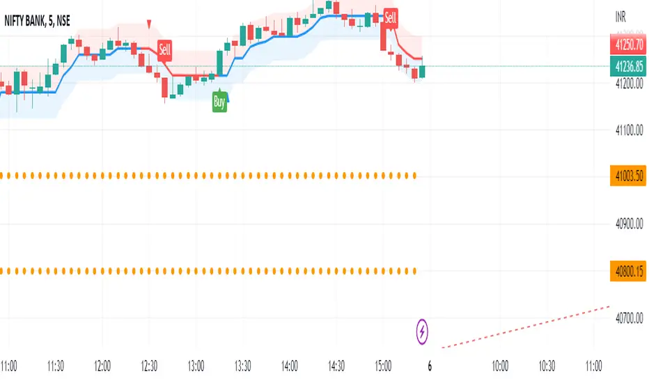
Strategy for UT Bot Alerts indicator Using the UT Bot alerts indicator by @QuantNomad, this strategy was designed for showing an example of how this indicator could be used, also, it has the goal to help some people from a group that use to use this indicator for their trading. Under any circumstance I recommend to use it without testing it before in real time.
Backtesting context: 2020-02-05 to 2023-02-25 of BTCUSD 4H by Tvc. Commissions: 0.03% for each entry, 0.03% for each exit. Risk per trade: 2.5% of the total account
For this strategy, 3 indicators are used:
UT Bot Alerts indicator by Quantnomad
One Ema of 200 periods for indicate the trend
Atr stop loss from Gatherio
Trade conditions:
For longs:
Close price is higher than Atr from UT Bot
Ema from UT Bot cross over Atr from UT Bot.
This gives us our long signal. Stop loss will be determined by atr stop loss (white point), break even(blue point) by a risk/reward ratio of 0.75:1 and take profit of 3:1 where half position will be closed. This will be showed as buy (open long position)
The other half will be closed when close price is lower than Atr and Ema from UT Bot cross under Atr. This will be showed as cl buy (close long position)
For shorts:
Close price is lower than Atr from UT Bot
Ema from UT Bot cross over Atr from UT Bot.
This gives us our short signal. Stop loss will be determined by atr stop loss (white point), break even(blue point) by a risk/reward ratio of 0.75:1 and take profit of 3:1 where half position will be closed. This will be showed as sell (open short position)
The other half will be closed when close price is higher than Atr and Ema from UT Bot cross over Atr. This will be showed as cl sell (close short position)
Risk management
For calculate the amount of the position you will use just a small percent of your initial capital for the strategy and you will use the atr stop loss for this.
Example: You have 1000 usd and you just want to risk 2,5% of your account, there is a long signal at price of 20,000 usd. The stop loss price from atr stop loss is 19,000. You calculate the distance in percent between 20,000 and 19,000. In this case, that distance would be of 5,0%. Then, you calculate your position by this way: (initial or current capital * risk per trade of your account) / (stop loss distance).
Using these values on the formula: (1000*2,5%)/(5,0%) = 500usd. It means, you have to use 500 usd for risking 2.5% of your account.
We will use this risk management for apply compound interest.
In settings, with position amount calculator, you can enter the amount in usd of your account and the amount in percentage for risking per trade of the account. You will see this value in green color in the upper left corner that shows the amount in usd to use for risking the specific percentage of your account.
Script functions
Inside of settings, you will find some utilities for display atr stop loss, break evens, positions, signals, indicators, etc.
You will find the settings for risk management at the end of the script if you want to change something. But rebember, do not change values from indicators, the idea is to not over optimize the strategy.
If you want to change the initial capital for backtest the strategy, go to properties, and also enter the commisions of your exchange and slippage for more realistic results.
In risk managment you can find an option called "Use leverage ?", activate this if you want to backtest using leverage, which means that in case of not having enough money for risking the % determined by you of your account using your initial capital, you will use leverage for using the enough amount for risking that % of your acount in a buy position. Otherwise, the amount will be limited by your initial/current capital
---> Do not forget to deactivate Trades on chart option in style settings for a cleaner look of the chart <---
Some things to consider
USE UNDER YOUR OWN RISK. PAST RESULTS DO NOT REPRESENT THE FUTURE.
DEPENDING OF % ACCOUNT RISK PER TRADE, YOU COULD REQUIRE LEVERAGE FOR OPEN SOME POSITIONS, SO PLEASE, BE CAREFULL AND USE CORRECTLY THE RISK MANAGEMENT
Do not forget to change commissions and other parameters related with back testing results!
Strategies for trending markets use to have more looses than wins and it takes a long time to get profits, so do not forget to be patient and consistent !
---> The strategy can still be improved, you can change some parameters depending of the asset and timeframe like risk/reward for taking profits, for break even, also the main parameters of the UT Bot Alerts <----