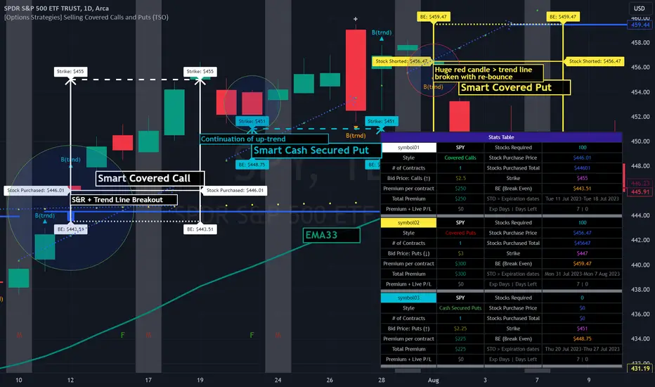
[Options Strategies] Selling Covered Calls and Puts (TSO) This trading indicator assists with traditional covered options trading strategies like Covered Calls, Covered Puts, and Cash Secured Puts. It also offers advanced features for trading options intelligently by utilizing options specific levels, such as BE (Break Even) and Strike (all visually shown on chart) in combination with S&R (Support and Resistance), Trend Lines, and other technical analysis tools such as MA (Moving Averages) and ATR Average True Range, all integrated within the indicator.
* Covered options approach over trading shares or options separately offers distinct advantages:
- Reduced Risk and Flexibility : Covered options strategy provides a more conservative approach by combining stock ownership with options trading. It reduces risk exposure compared to buying options outright or trading shares alone. Additionally, it offers flexibility in various market conditions.
- Profitability in Sideways Markets: Covered options allow for profitability in scenarios where the stock price is either moving optimally or remaining sideways. In contrast, just holding stocks might not yield significant gains in a sideways market, and buying options can result in losses due to time decay.
- Protection Against Price Movements: In covered options, if the stock price goes against the trade, the loss is mitigated by the premium received from selling the options. This provides a level of protection compared to other trading strategies where losses can accumulate more rapidly.
==============================================================
Strategies / Visual Examples:
---------------------------------------------------------------------------
---------------------------------------------------------------------------
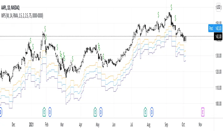
Up to 3 Symbols can be monitored at the same time with alerts for each Symbol and a Stats Table. To see Symbol's visuals (Date Range, Strike, BE, etc.) - the chart has to be loaded with that Symbol. Here is an example of trading multiple stocks at same layout on different charts trading AAPL, BAC and TSLA.
---------------------------------------------------------------------------
---------------------------------------------------------------------------
An example of a Smart Covered Calls trading SPY.
STRATEGY EXPLANATION:
* Trade Open Trigger (Bullish/Sideway)
>>> S&R (Support and Resistance) or Trend Line broken, bounced off or simply near (if price is near/slightly crossing S&R/Trend Line > a bounce often takes place)
>>> Confirmation by additional TA (Technical Analysis) tools.
>>> EXAMPLE: Broken Resistance combined with a Trend Line up-bounce, confirmed by bullish 200EMA.
* TP (Take-Profit)
>>> Contracts Expire at Expiration date: Premium received for selling contracts kept.
>>> Assignment: Premium received for selling contracts kept + stock assigned/sold at a higher price than it was purchased.
* BE/SL (Break Even Stop-Loss) |
>>> BE/SL hit: stock sold at a slight loss with options contracts bought out (BTC - Buy to Close) at a lower price than initially sold (since price went down and these are calls), so technically the loss is reduced by the partial Premium still kept from initially sold contracts at trade open.
>>> Increasing the BE/SL distance: for wider BE/SL > Bid Price needs to be increased:
- Set longer Expiration date.
- Set closer Strike price.
NOTE: With longer Expiration date and closer Strike, chances of assignment increase as well. It's best to find an optimal level, where BE/SL is behind a Support/Resistance level and/or an established trend line and/or Large Length Moving Average, yet not extremely far away.
---------------------------------------------------------------------------
---------------------------------------------------------------------------
An example of a Smart Covered Puts trading SPY.
STRATEGY EXPLANATION:
* Trade Open Trigger (Bearish/Sideway)
>>> S&R (Support and Resistance) or Trend Line broken, bounced off or simply near (if price is near/slightly crossing S&R/Trend Line > a bounce often takes place)
>>> Confirmation by additional TA (Technical Analysis) tools.
>>> EXAMPLE: Broken Resistance combined with a Trend Line down-bounce, confirmed by bearish 200EMA.
* TP (Take-Profit)
>>> Contracts Expire at Expiration date: Premium received for selling contracts kept.
>>> Assignment: Premium received for selling contracts kept + stock assigned/bought-to-cover at a lower price than it was shorted.
* BE/SL (Break Even Stop-Loss) |
>>> BE/SL hit: stock bought-to-cover at a slight loss with options contracts bought out (BTC - Buy to Close) at a lower price than initially sold (since price went up and these are puts), so technically the loss is reduced by the partial Premium still kept from initially sold contracts at trade open.
>>> Increasing the BE/SL distance: for wider BE/SL > Bid Price needs to be increased:
- Set longer Expiration date.
- Set closer Strike price.
NOTE: With longer Expiration date and closer Strike, chances of assignment increase as well. It's best to find an optimal level, where BE/SL is behind a Support/Resistance level and/or an established trend line and/or Large Length Moving Average, yet not extremely far away.
---------------------------------------------------------------------------
---------------------------------------------------------------------------
An example of a Smart Secured Cash Puts trading SPY.
STRATEGY EXPLANATION:
* Trade Open Trigger (Bullish/Sideway)
>>> Bullish steady trend.
>>> Confirmation by additional TA (Technical Analysis) tools.
>>> EXAMPLE: Slowly rising price action above 200EMA.
* TP (Take-Profit)
>>> Early BTC: BTC (Buy to Close) before Expiration date if options premium/contract price already reduced by at least 50-90% (the reduced price is the profit, if premium lost 90% - only 10% will need to be paid to buy options out to close the trade) and if the stock price is nearing Resistance, Trend Line or big length moving average (like 200EMA) as a bounce may happen or even a potential reverse of the trend. If there is no trend reversal or a small correction bounce occurs, with further trend continuation > another Cash Secured Puts trade can be opened with new Expiration date and Strike.
>>> Contracts Expire at Expiration date: Premium received for selling contracts kept, considering the Strike was never hit.
>>> Assignment with stock closing below Strike and above/near BE (Break Even): Premium received for selling contracts kept. NOTE: It is best to get rid of the stock ASAP to then open a new Cash Secured Puts trade with lower Strike and a new Expiration date.
* BE/SL (Break Even Stop-Loss) |
>>> BE/SL hit: contracts bought out (BTC - Buy to Close) at a higher price than initially sold (since price went down and these are puts), the amount/difference in current contract price is the loss (as premium received + contract price increase is the total cost, which will have to be paid to buy the countracts out).
>>> Increasing the BE/SL distance: for wider BE/SL > Bid Price needs to be increased:
- Set longer Expiration date.
- Set closer Strike price.
NOTE: With longer Expiration date and closer Strike, chances of assignment increase as well. It's best to find an optimal level, where BE/SL is behind a Support/Resistance level and/or an established trend line and/or Large Length Moving Average, yet not extremely far away.
---------------------------------------------------------------------------
---------------------------------------------------------------------------
An example of Options Wheel strategy trading TQQQ. See how Strike and BE (Break Even) hits are displayed every time they occur.
STRATEGY EXPLANATION:
* Trade Open Trigger (Bullish/Sideway)
>>> Options Wheel strategy combines Cash Secured Puts with Covered Calls, so a steady bullish trend is preferred with lower volatility.
>>> It's best to start with Cash Secured Puts until assignment hits (stocks purchased), then switch to Covered Calls until assignment hits (stocks sold) and so on.
* TP (Take-Profit)
>>> Contracts Expire at Expiration date: Premium received for selling contracts kept.
>>> Assignment: Premium received for selling contracts kept. Stock is assigned (purchased if Cash Secured Puts were sold | sold if Covered Calls were sold ).
* BE/SL (Break Even Stop-Loss)
>>> Assignment is the stop-loss for this strategy, which ends current trade and starts next one. It is not a direct loss, but could result a long unrealized losses if after stock purchase assignment it goes down for a while or even a complete loss if low-cap company is used and it goes out of business.
>>> BE/SL distance can still be increased/kept optimal: for wider BE/SL > Bid Price needs to be increased:
- Set longer Expiration date.
- Set closer Strike price.
NOTE: With longer Expiration date and closer Strike, chances of assignment increase as well. It's best to find an optimal level, where BE/SL is behind a Support/Resistance level and/or an established Trend Line and/or Large Length Moving Average, yet not extremely far away.
| 3.0_wheel_strategy_tqqq_example.png
===========================================================================
Trading open/close/TP/SL labels, plots and colors explanations:
---------------------------------------------------------------------------
There are 3 approaches: Cashed Secured Puts, Covered Puts, Covered Calls. Here is an example showing all 3 (the Strikes, Bid prices, Expirations were chosen realistically).
>>> There are 3 symbol templates, the color can be changed for each and each symbol template can be unchecked to be fully hidden or all 3 can be used.
>>> Strike: dashed horizontal line plotted at chosen Strike, if Strike is hit within the Date Range - there will be a label shown.
>>> BE (Break Even): dotted horizontal line plotted at calculated BE, if BE is hit within the Date Range - there will be a label shown.
>>> Stock Purchased: solid horizontal line plotted at input price at which the stock was purchased.
>>> Date Range (STO >>> Expiration ): vertical lines with arrows (arrows direction is based on the approach), which connect Strike, BE (Break Even) and Stock Purchased creating an square/rectangle of the whole trade, making it easy to see everything at once.
>>> Stats Table: shows all the necessary data for each symbol.
===========================================================================
GLOBAL SETTINGS ///////////////////////////////////////////////////////////
---------------------------------------------------------------------------
>>> Show: week divider vertical lines: Will show vertical divider lines separating each week.
>>> Show: Mondays and Fridays: Will show M - for Monday, F - for Friday, T - for Tuesday (Tuesday will be shown if there is a Holiday on Monday)
---------------------------------------------------------------------------
OPTIONS SETUP: SYMBOL0X /////////////////////////////////////////////////// | (identical for all 3 symbols)
---------------------------------------------------------------------------
>>> Symbol0X | Show Table: Turns on symbol01, all visuals on chart, calculations, etc. Table can be separately hidden if desired.
>>> Label Size: Size of the labels on chart showing Strike, BE (Break Even), etc.
>>> Label Color: Color for all symbol0X labels.
>>> Text Color: Text color for all symbol0X labels.
>>> Options Trading Style: 1)Covered Calls: Bullish-sideways market approach (need to own 100 shares of stock per each contract sold), Strike price has to be set above the current stock price | 2)Covered Puts: Bearish-sideways market approach (need to own 100 shares of stock per each contract sold), Strike price has to be set below the current stock price | 3)Cash Secured Puts: Bullish-sideways approach (need to have enough cash to acquire shares at Strike price if hit), Strike price has to be set below the current stock price.
>>> # of contracts sold (1 contract > 100shares): # of contracts sold per trade, for Covered Calls and Covered Puts, every contract must be backed up by 100shares of the underlying stock.
>>> Price per 1 contract (Bid): Premium received per each contract sold.
>>> Strike Price.
>>> Stock Purchase Price: Stock purchase price (NOTE: This is only for Covered Call and Covered Puts, for Secured Cash Puts - stock is only purchased if at Expiration it closes beyond Strike price).
>>> STO (Sell to Open) Date: date at which the contracts were sold and Premium received.
>>> Exp (Expiration) Date: date at which contracts expire, if price never breaks the Strike at Expiration - contracts become worthless!
>>> Alert/Label: Futures Expire Soon: With this setting turned on, an Alert will trigger and a Label will be shown at opening of the first candle bar on the Expiration date. It will certainly be before the end of the day, however depending on the chart TimeFrame during alert creation - it may trigger at a different time. For Example: On a Daily chart TimeFrame SPY (S&P500) will trigger such alert at 9:30AM ET. ||| NOTE: Due to difference in timezones - the solid lines representing the STO >>> Exp range may be off by 1 business day from the date input in the indicator Settings > Inputs, so double check and calibrate the date by setting it 1 day behind/ahead from actual dates so that Alert is received on the actual Expiration date.
>>> Strike price Broken - Style: 'Close': Show/Alert Strike price broken only once candle bar is closed | 'Live': Show/Alert Strike price broken immediately once it happens, before candle bar is closed.
>>> Show: Strike price Broken: will show a label near candle bar breaking the Strike price.
>>> Alert: Strike price Broken: will alert at price breaking the Strike price.
>>> BE (Break Even) price Broken - Alert Style: 'Close': Show/Alert BE (Break Even) price broken only once candle bar is closed | 'Live': Show/Alert BE (Break Even) price broken immediately once it happens, before candle bar is closed.
>>> Show: BE (Break Even) price Broken: will show a label near candle bar breaking the BE price.
>>> Alert: BE (Break Even) price Broken: will alert at price breaking the BE price.
---------------------------------------------------------------------------
TA: TREND LINES ///////////////////////////////////////////////////////////
---------------------------------------------------------------------------
>>> Trend Lines - Uptrend/downtrend colors
>>> Show: Trend Lines: Show/Hide trend lines
>>> Show: Trend Line Breaks: Show/Hide labels where trend lines were broken
>>> Alert: Trend Line Breaks: Alert when trend line is broken
>>> Trend Lines - Search - Left Bars / Trend Lines - Search - Right Bars: how many candle bars will be used to calculate Trend Lines, the bigger the number > the more precise and less amount of trend lines will be found
>>> Trend Lines - Extend Setting
---------------------------------------------------------------------------
TA: S&R (SUPPORT AND RESISTANCE) //////////////////////////////////////////
---------------------------------------------------------------------------
>>> S&R (Support and Resistance) - Support/Resistance colors.
>>> Show: S&R (Support and Resistance) Top/Bottom Levels.
>>> Show: S&R (Support and Resistance) Top/Bottom Level Breaks: Show/Hide labels where support/resistance levels were broken
>>> Alert: S&R (Support and Resistance) Top/Bottom Level Breaks: Alert when S&R (Support and Resistance) level is broken
>>> S&R (Support and Resistance) - Search - Left Bars / S&R (Support and Resistance) - Search - Right Bars: how many candle bars will be used to calculate S&R (Support & Resistance) Levels, the bigger the number > the more precise and less amount of support and resistance levels will be found.
>>> S&R Search - Custom Resolution: This is a custom timeframe setting specifically for S&R Search, it disregards current chart timeframe. This is great to use for scalping, for example: with main chart set to 1min and the custom timeframe set to 3min or 5min - there will be stronger support/resistance levels with more detailed price action.
---------------------------------------------------------------------------
TA: ADDITIONAL TOOLS //////////////////////////////////////////////////////
>>> Show - MA (Moving Average).
>>> Show - ATR (Average True Range).
---------------------------------------------------------------------------
---------------------------------------------------------------------------
STATS TABLE ///////////////////////////////////////////////////////////////
Stats Table displays all the necessary date about each options setup.
>>> Table positioning
---------------------------------------------------------------------------
===========================================================================
Adding Alerts in TradngView
---------------------------------------------------------------------------
-Add indicator to chart and make sure to check/uncheck which alerts are required, then simply create it.
-Right-click anywhere on the TradingView chart
-Click on Add alert
-Condition: Select this indicator by it’s name
-Immediately below, change it to "alert() function calls only"
-Expiration: Open-ended (that may require higher tier TradingView account, otherwise the alert will need to be occasionally re-triggered)
-Alert name: Whatever you desire
-Hit “Create”
-Note: If you change ANY Settings within the indicator – you must DELETE the current alert and create a new one per steps above, otherwise it will continue triggering alerts per old Settings!
===========================================================================
If you have any questions or issues with the indicator, please message me directly via TradingView.
---------------------------------------------------------------------------
Good Luck! (NOTE: Trading is very risky, past performance is not necessarily indicative of future results, so please trade responsibly!)
Optionsstrategies
BetaBeta , also known as the Beta coefficient, is a measure that compares the volatility of an individual underlying or portfolio to the volatility of the entire market, typically represented by a market index like the S&P 500 or an investible product such as the SPY ETF (SPDR S&P 500 ETF Trust). A Beta value provides insight into how an asset's returns are expected to respond to market swings.
Interpretation of Beta Values
Beta = 1: The asset's volatility is in line with the market. If the market rises or falls, the asset is expected to move correspondingly.
Beta > 1: The asset is more volatile than the market. If the market rises or falls, the asset's price is expected to rise or fall more significantly.
Beta < 1 but > 0: The asset is less volatile than the market. It still moves in the same direction as the market but with less magnitude.
Beta = 0: The asset's returns are not correlated with the market's returns.
Beta < 0: The asset moves in the opposite direction to the market.
Example
A beta of 1.20 relative to the S&P 500 Index or SPY implies that if the S&P's return increases by 1%, the portfolio is expected to increase by 12.0%.
A beta of -0.10 relative to the S&P 500 Index or SPY implies that if the S&P's return increases by 1%, the portfolio is expected to decrease by 0.1%. In practical terms, this implies that the portfolio is expected to be predominantly 'market neutral' .
Calculation & Default Values
The Beta of an asset is calculated by dividing the covariance of the asset's returns with the market's returns by the variance of the market's returns over a certain period (standard period: 1 years, 250 trading days). Hint: It's noteworthy to mention that Beta can also be derived through linear regression analysis, although this technique is not employed in this Beta Indicator.
Formula: Beta = Covariance(Asset Returns, Market Returns) / Variance(Market Returns)
Reference Market: Essentially any reference market index or product can be used. The default reference is the SPY (SPDR S&P 500 ETF Trust), primarily due to its investable nature and broad representation of the market. However, it's crucial to note that Beta can also be calculated by comparing specific underlyings, such as two different stocks or commodities, instead of comparing an asset to the broader market. This flexibility allows for a more tailored analysis of volatility and correlation, depending on the user's specific trading or investment focus.
Look-back Period: The standard look-back period is typically 1-5 years (250-1250 trading days), but this can be adjusted based on the user's preference and the specifics of the trading strategy. For robust estimations, use at least 250 trading days.
Option Delta: An optional feature in the Beta Indicator is the ability to select a specific Delta value if options are written on the underlying asset with Deltas less than 1, providing an estimation of the beta-weighted delta of the position. It involves multiplying the beta of the underlying asset by the delta of the option. This addition allows for a more precise assessment of the underlying asset's correspondence with the overall market in case you are an options trader. The default Delta value is set to 1, representing scenarios where no options on the underlying asset are being analyzed. This default setting aligns with analyzing the direct relationship between the asset itself and the market, without the layer of complexity introduced by options.
Calculation: Simple or Log Returns: In the calculation of Beta, users have the option to choose between using simple returns or log returns for both the asset and the market. The default setting is 'Simple Returns'.
Advantages of Using Beta
Risk Management: Beta provides a clear metric for understanding and managing the risk of a portfolio in relation to market movements.
Portfolio Diversification: By knowing the beta of various assets, investors can create a balanced portfolio that aligns with their risk tolerance and investment goals.
Performance Benchmarking: Beta allows investors to compare an asset's risk-adjusted performance against the market or other benchmarks.
Beta-Weighted Deltas for Options Traders
For options traders, understanding the beta-weighted delta is crucial. It involves multiplying the beta of the underlying asset by the delta of the option. This provides a more nuanced view of the option's risk relative to the overall market. However, it's important to note that the delta of an option is dynamic, changing with the asset's price, time to expiration, and other factors.

[BCT] Option Pricing via Markov Chain Monte Carlo SimulationOverview:
This script offers a toolkit for quantitative options trading, using Monte Carlo simulations based on actual historical returns to model potential future price paths for underlying assets. A range of metrics related to options trading are also provided.
Monte Carlo Simulations:
The script employs Monte Carlo simulations to model future price paths based on the historical returns of the underlying asset. These simulated paths are represented as parabolas at the 2-sigma, 25th percentile, and median levels for quick reference.
Methodologies:
For calculating options prices at At-the-Money (or any user-selected strike), two methodologies are used:
Simple Averaging: Takes the mean of the simulated asset price paths.
Kernel Density Estimation (KDE): Applied to the simulated asset price paths to produce a smoothed estimate of its probability density function, thereby aiding in a more nuanced option price calculation.
Bootstrap Resampling:
Bootstrap resampling is specifically applied to the simulated asset price paths to generate an estimate of the standard deviation of the options prices. Note that while bootstrap methods are employed, they serve as statistical tools and do not guarantee statistical reliability.
Metrics Displayed:
Model-Estimated At-the-Money (or selected strike) Straddle Price
Model-Estimated At-the-Money (or selected strike) Call Price
Model-Estimated At-the-Money (or selected strike) Put Price
Model-Estimated Standard deviation for Option Prices from simulated price paths
Underlying Monte Carlo Simulation Results (represented as parabolas at the 2 sigma, 25 percentile and median)
This is not financial advice. Use at your own risk.
Disclaimer: Options trading carries a high level of risk and may not be suitable for all investors. This script is intended to serve as an educational tool and should not be considered financial advice. While designed to aid in decision-making, the script's indicators are not guarantees of performance or outcomes. Always conduct your own due diligence before making trading decisions.

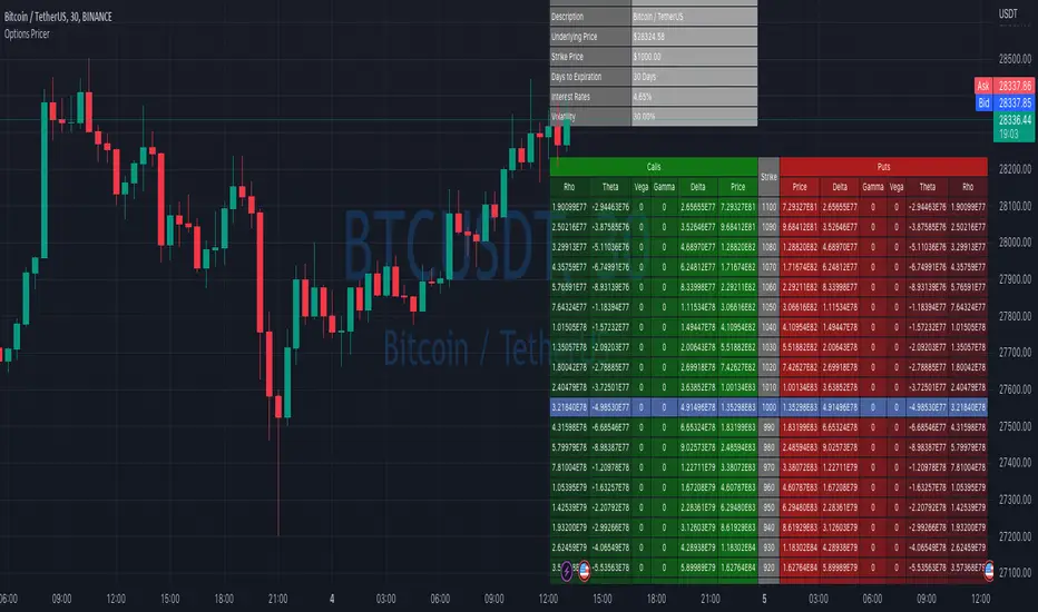
Options Price CalculatorIn the team, we continue to explore and expand the boundaries of TradingView.
For now, there is not much an options trader can do with options in TradingView.
We wanted to change that and created a simple option pricer.
You can set up in parameters a set of strikes, implied volatility, and days to expiry.
The indicators will take a risk-free rate from US01Y and the underlying price from your current chart.
It will compute prices and greeks for both put and call options.
Thanks to @MUQWISHI for helping code it.
Disclaimer
Please remember that past performance may not indicate future results.
Due to various factors, including changing market conditions, the strategy may no longer perform as well as in historical backtesting.
This post and the script don’t provide any financial advice.
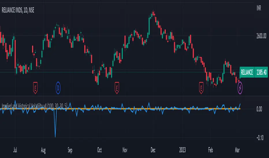
Implied and Historical Volatility v4There is a famous option strategy📊 played on volatility📈. Where people go short on volatility, generally, this strategy is used before any significant event or earnings release. The basic phenomenon is that the Implied Volatility shoots up before the event and drops after the event, while the volatility of the security does not increase in most of the scenarios. 💹
I have tried to create an Indicator using which you
can analyse the historical change in Implied Volatility Vs Historic Volatility.
To get a basic idea of how the security moved during different events.
Notes:
a) Implied Volatility is calculated using the bisection method and Black 76 model option pricing model.
b) For the risk-free rate I have fetched the price of the “10-Year Indian Government Bond” price and calculated its yield to be used as our Risk-Free rate.
Jerry J8 30-123 Spy Dashboard ProPlease watch the J8 Scalping Tutorial Video below for a walkthrough on how these indicators work.
This script is used in conjunction with Jerry J8 30-123 SPY Scalping PRO” Indicator(which creates the buy and sell orders as a strategy). The Dashboard shows the 4 main criteria statuses from the strategy. I find the dashboard makes scalping the SPY much easier.
This study project is designed for scalping options that expire daily with bull put and bear call credit spreads on a 3 minute chart. The name 30_123 is a reference to 4 main criteria being met to give a green light for a potential trade. The criteria:
* 30 = 30 minute trend
* 1 = 3 minute trend
* 2 = Moving average criteria
* 3 = RSI criteria
4 = Secondary trend. Bonus if in sync but not a requirement.
* The strategy also utilizes momentum as a criteria but this is not shown on the dashboard.
This indicator is designed to trade options that expire daily including the SPY, IWM, QQQ, and NDX. However, it can be used with multiple symbols on a 3 minute chart.
When the 30_123 conditions are all green with all criteria are met a bull signal is created.
When the 30_123 conditions are all red with all criteria are met a bear signal is created.
This study is the dashboard that is designed to show how the main J8 strategy indicator is working and it shows which criteria have been met. Additionally there are multiple user INPUTS that you can adjust for the 4 main criteria plus inputs to help you with your credit spread criteria.
For example, if the SPY is at 400 we could have an order to sell a BULL PUT CREDIT SPREAD and I would likely sell the 398p and buy the 397p; The 398p delta would be approximately -.2. The spread position profits with any close over 398 and/or can be closed early with a bullish price move. IMPORTANT: If the SPY closed the day at $399 on the chart it would look like a loss based on the buy and sell orders but the spread would be a full profit since the close was above 398.
---- IRON CONDOR
For the SPY ticker only an iron condor label is generated when the SPY is trading sideways and meets specified criteria. When the criteria is met the Iron Condor label appears and it provides a recommendation for what option to buy and sell. The iron condor recommendations can be adjusted with user inputs.
This Indicator dashboard shows the criteria labels and colors the criteria as green if bullish and red if bearish. When the criteria are not met the dashboard shows “NO CLEAR SIGNAL”. There is also a label that shows whether you are looking for bullish or bearish positions based on the 30 minute trend.
The chart shown on the indicator is the RSI and for this indicator an RSI over 50 is bullish and under 50 is bearish. The line color shows the RSI trend. RSI OB (overbought) and OS (oversold) areas are shaded. The RSI can remain in an OB or OS state for a prolonged period and while some people use OB and OS as a reversal signal I use it as a strong trend indication and recognize it will not last forever. You can SET the OB and OS levels with inputs.
---- USER INPUTS
Paint Bars: Turns on/off the candle coloring. Default is OFF.
Iron Condor Settings: Defaults are what I use and can be used as a guide.
Criteria: Trend, moving averages, and RSI settings can all be adjusted.
---- SETUP & HINTS
Add "Jerry J8 30-123 SPY Scalping PRO” indicator to show bull and bear signals
Add "Jerry J8 MACD Optimal Entry Zone” indicator to show best MACD range for entry
I also like to add "Jerry Momentum Dream" indicator to see the momentum
With this indicator we’re looking for the 30, 1, 2, and 3 criteria to be met which increases our likelihood of success. IMPORTANT. Never automatically enter a position without reviewing the other indicators and drawing your own conclusions. You want to choose the entries that are the most appealing to you that take into account volume, time of day, and risk/reward. Positions should be closed based on your risk/reward goals.
Indicators are not a magic pill and should be used to support trading decisions, not to make them for you. Past performance is not a guarantee of future returns. The results of individual stocks/indexes with any strategy do not constitute proof they will repeat in the future.
DISCLAIMER: The information contained in our scripts/indicators/ideas does not constitute financial advice or a solicitation to buy or sell any securities of any type. Trading and investing in the stock market and cryptocurrencies involves substantial risk of loss and is not suitable for every investor. I’m NOT a financial adviser. All trading strategies are used at your own risk.
Please Use the AUTHOR’s INSTRUCTIONS link below for more information.
NOTE: The PERFORMANCE SUMMARY below does not accurately reflect the trading strategy because the entry orders generated in the strategy are based on the stock price and our actual order is a credit spread that is profitable even if the price moves against us a little bit. What could show as a loss in the strategy could be a profit in the credit spread.

VolatilityCone by ImpliedVolatilityThis volatility cone draws the implied volatility as standard deviations from a measurement date.
For best results set measurement date to high volume bars.
How to use:
1) Select VolatilityCone from Indicators
2) Click to the chart to set the measurement date
3) Determine the impliedvolatility for the measurement date of your symbol
e.g.
For S&P500 use VIX value at measurement date for implied volatility

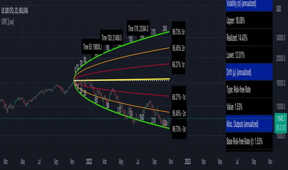
Volatility Cone [Loxx]When it comes to forecasting volatility, it seems that the old axiom about weather is applicable: "Everyone talks about it, but no one can do much about it!" Volatility cones are a tool that may be useful in one’s attempt to do something about predicting the future volatility of an asset.
A "volatility cone" is a plot of the range of volatilities within a fixed probability band around the true parameter, as a function of sample length. Volatility cone is a visualization tool for the display of historical volatility term structure. It was introduced by Burghardt and Lane in early 1990 and is popular in the option trading community. This is mostly a static indicator due to processor load and is restricted to the daily time frame.
Why cones?
When we enter the options arena, in an effort to "trade volatility," we want to be able to compare current levels of implied volatility with recent historical volatility in an effort to assess the relative value of the option(s) under consideration Volatility cones can be an effective tool to help us with this assessment. A volatility cone is an analytical application designed to help determine if the current levels of historical or implied volatilities for a given underlying, its options, or any of the new volatility instruments, such as VolContractTM futures, VIX futures, or VXX and VXZ ETNs, are likely to persist in the future. As such, volatility cones are intended to help the user assess the likely volatility that an underlying will go on to display over a certain period. Those who employ volatility cones as a diagnostic tool are relying upon the principle of "reversion to the mean." This means that unusually high levels of volatility are expected to drift or move lower (revert) to their average (mean) levels, while relatively low volatility readings are expected to rise, eventually, to more "normal" values.
How to use
Suppose you want to analyze an options contract expiring in 3-months and this current option has an current implied volatility 25.5%. Suppose also that realized volatility (y-axis) at the 3-month mark (90 on the x-axis) is 45%, median in 35%, the 25th percentile is 30%, and the low is 25%. Comparing this range to the implied volatility you would maybe conclude that this is a relatively "cheap" option contract. To help you visualize implied volatility on the chart given an expiration date in bars, the indicator includes the ability to enter up to three expirations in bars and each expirations current implied volatility
By ascertaining the various historical levels of volatility corresponding to a given time horizon for the options futures under consideration, we’re better prepared to judge the relative "cheapness" or "expensiveness" of the instrument.
Volatility options
Close-to-Close
Close-to-Close volatility is a classic and most commonly used volatility measure, sometimes referred to as historical volatility .
Volatility is an indicator of the speed of a stock price change. A stock with high volatility is one where the price changes rapidly and with a bigger amplitude. The more volatile a stock is, the riskier it is.
Close-to-close historical volatility calculated using only stock's closing prices. It is the simplest volatility estimator. But in many cases, it is not precise enough. Stock prices could jump considerably during a trading session, and return to the open value at the end. That means that a big amount of price information is not taken into account by close-to-close volatility .
Despite its drawbacks, Close-to-Close volatility is still useful in cases where the instrument doesn't have intraday prices. For example, mutual funds calculate their net asset values daily or weekly, and thus their prices are not suitable for more sophisticated volatility estimators.
Parkinson
Parkinson volatility is a volatility measure that uses the stock’s high and low price of the day.
The main difference between regular volatility and Parkinson volatility is that the latter uses high and low prices for a day, rather than only the closing price. That is useful as close to close prices could show little difference while large price movements could have happened during the day. Thus Parkinson's volatility is considered to be more precise and requires less data for calculation than the close-close volatility. One drawback of this estimator is that it doesn't take into account price movements after market close. Hence it systematically undervalues volatility. That drawback is taken into account in the Garman-Klass's volatility estimator.
Garman-Klass
Garman Klass is a volatility estimator that incorporates open, low, high, and close prices of a security.
Garman-Klass volatility extends Parkinson's volatility by taking into account the opening and closing price. As markets are most active during the opening and closing of a trading session, it makes volatility estimation more accurate.
Garman and Klass also assumed that the process of price change is a process of continuous diffusion (geometric Brownian motion). However, this assumption has several drawbacks. The method is not robust for opening jumps in price and trend movements.
Despite its drawbacks, the Garman-Klass estimator is still more effective than the basic formula since it takes into account not only the price at the beginning and end of the time interval but also intraday price extremums.
Researchers Rogers and Satchel have proposed a more efficient method for assessing historical volatility that takes into account price trends. See Rogers-Satchell Volatility for more detail.
Rogers-Satchell
Rogers-Satchell is an estimator for measuring the volatility of securities with an average return not equal to zero.
Unlike Parkinson and Garman-Klass estimators, Rogers-Satchell incorporates drift term (mean return not equal to zero). As a result, it provides a better volatility estimation when the underlying is trending.
The main disadvantage of this method is that it does not take into account price movements between trading sessions. It means an underestimation of volatility since price jumps periodically occur in the market precisely at the moments between sessions.
A more comprehensive estimator that also considers the gaps between sessions was developed based on the Rogers-Satchel formula in the 2000s by Yang-Zhang. See Yang Zhang Volatility for more detail.
Yang-Zhang
Yang Zhang is a historical volatility estimator that handles both opening jumps and the drift and has a minimum estimation error.
We can think of the Yang-Zhang volatility as the combination of the overnight (close-to-open volatility ) and a weighted average of the Rogers-Satchell volatility and the day’s open-to-close volatility . It considered being 14 times more efficient than the close-to-close estimator.
Garman-Klass-Yang-Zhang
Garman Klass is a volatility estimator that incorporates open, low, high, and close prices of a security.
Garman-Klass volatility extends Parkinson's volatility by taking into account the opening and closing price. As markets are most active during the opening and closing of a trading session, it makes volatility estimation more accurate.
Garman and Klass also assumed that the process of price change is a process of continuous diffusion (geometric Brownian motion). However, this assumption has several drawbacks. The method is not robust for opening jumps in price and trend movements.
Despite its drawbacks, the Garman-Klass estimator is still more effective than the basic formula since it takes into account not only the price at the beginning and end of the time interval but also intraday price extremums.
Researchers Rogers and Satchel have proposed a more efficient method for assessing historical volatility that takes into account price trends. See Rogers-Satchell Volatility for more detail.
Exponential Weighted Moving Average
The Exponentially Weighted Moving Average (EWMA) is a quantitative or statistical measure used to model or describe a time series. The EWMA is widely used in finance, the main applications being technical analysis and volatility modeling.
The moving average is designed as such that older observations are given lower weights. The weights fall exponentially as the data point gets older – hence the name exponentially weighted.
The only decision a user of the EWMA must make is the parameter lambda. The parameter decides how important the current observation is in the calculation of the EWMA. The higher the value of lambda, the more closely the EWMA tracks the original time series.
Standard Deviation of Log Returns
This is the simplest calculation of volatility . It's the standard deviation of ln(close/close(1))
Sampling periods used
5, 10, 20, 30, 60, 90, 120, 150, 180, 210, 240, 270, 300, 330, and 360
Historical Volatility plot
Purple outer lines: High and low volatility values corresponding to x-axis time
Blue inner lines: 25th and 75th percentiles of volatility corresponding to x-axis time
Green line: Median volatility values corresponding to x-axis time
White dashed line: Realized volatility corresponding to x-axis time
Additional things to know
Due to UI constraints on TradingView it will be easier to visualize this indicator by double-clicking the bottom pane where it appears and then expanded the y- and x-axis to view the entire chart.
You can click on each point on the graph to see what the volatility of that point is.
Option expiration dates will show up as large dots on the graph. You can input your own values in the settings.

Variety Distribution Probability Cone [Loxx]Variety Distribution Probability Cone forecasts price within a range of confidence using Geometric Brownian Motion (GBM) calculated using selected probability distribution, volatility, and drift. Below is detailed explanation of the inner workings of the indicator and the math involved. While normally this indicator would be used by options traders, this can also be used by regular directional traders who wish to observe a forecast of the confidence interval of possible prices over time.
What is a Random Walk
A random walk is a path which consists of a set of random steps. The starting point is zero and following movement may be one step to the left or to the right with equal probability. In the random walk process, there is no observable trend or pattern which are followed by the objects that is the movements are completely random. That is why the prices of a stock as it moves up and down can be modeled by random a walk process.
Stock Prices and Geometric Brownian Motion
Brownian motion, as first conceived by the botanist Robert Brown (1827), is a mathematical model used to describe random movements of small particles in a fluid or gas. These random movements are observed in the stock markets where the prices move up and down, randomly; hence, Brownian motion is considered as a mathematical model for stock prices.
P(exp(lnS0 + (mu + 1/2*sigma^2)t - z(0.05)*sigma*t^0.5) <= St <= exp(lnS0 + (mu + 1/2*sigma^2)t + z(0.05)*sigma*t^0.5)) = 0.95
Probability Distributions
Typically the normal distribution is used, but for our purposes here we extend this to Student t-distribution, Cauchy, Gaussian KDE, and Laplace
Student's t-Distribution
The probability density function of the Student’s t distribution is given by
g(x) = (L(v+1)/2) / L(v/2) * 1 / L(sqrt(v)) * (1 + x^2/v) ^ (-(v+1)/2)
with v degrees of freedom and v >= 0, denoted by X ~ t(v). The mean is 0 and the variance is v/(v-2). It is known that as v tends to infinity, the Student’s t-distribution tends to a standard normal probability density function, which has a variance of one. Blattberg and Gonedes were the first to propose that stock returns could be modeled by this distribution. (Blattberg and Gonedes, 1974) Platen and Sidorowicz later reaffirmed these findings.(Platen and Rendek, 2007) Finally, Cassidy, Hamp, and Ouyed used these findings to derive the Gosset formula, which is the Student t version of the Black-Scholes model.(Cassidy et al., 2010) They found that v = 2.65 provides the best fit when looking at the past 100 years of returns. They realized that as markets become more turbulent, the degrees of freedom should be adjusted to a smaller value.(Cassidy et al., 2010)
Cauchy Distribution
The probability density function of the Cauchy distribution is given by
f(x) = 1 / (theta*pi*(1 + ((x-n)/v)))
where n is the location parameter and theta is the scale parameter, for -infinity < x < infinity and is denoted by X ~ CAU(L,v). This model is similar to the normal distribution in that it is symmetric about zero, but the tails are fatter. This would mean that the probability of an extreme event occurring lies far out in the distributions tail. Using a crude example, if the normal distribution gave a probability of an extreme event occurring of 0.05% and the “best case” scenario of this event occurring 300 years, then using the Cauchy distribution one would find that the probability of occurring would be around 5% and now the “best case” scenario might have been reduced to only 63 years. Thus giving extreme events more of a likelihood of occurring. The mean, variance, and higher order moments are not defined (they are infinite); this implies that n and theta cannot be related to a mean and standard deviation. The Cauchy distribution is related to the Student’s t distribution T ~ CAU(1,0) when v = 1. In 1963, Benoit Mandelbrot was the first to suggest that stock returns follow a stable distribution, in particular, the Cauchy distribution.(Mandelbrot, 1963) His work was validated by Eugene Fama in 1965.(Fama, 1965) Recent research by Nassim Taleb came to the same conclusion as Mandelbrot, saying that stock returns follow a Cauchy distribution, as reported in his New York Times best-seller book “The Black Swan”.(Taleb, 2010)
Laplace Distribution
In probability theory and statistics, the Laplace distribution is a continuous probability distribution named after Pierre-Simon Laplace. It is also sometimes called the double exponential distribution, because it can be thought of as two exponential distributions (with an additional location parameter) spliced together along the abscissa, although the term is also sometimes used to refer to the Gumbel distribution. The difference between two independent identically distributed exponential random variables is governed by a Laplace distribution, as is a Brownian motion evaluated at an exponentially distributed random time. Increments of Laplace motion or a variance gamma process evaluated over the time scale also have a Laplace distribution.
The probability density function of the Cauchy distribution is given by
f(x) = 1/2b * exp(-|x-µ|/b)
Here, µ is a location parameter and b > 0, which is sometimes referred to as the "diversity", is a scale parameter. If µ = 0 and b=1, the positive half-line is exactly an exponential distribution scaled by 1/2.
The probability density function of the Laplace distribution is also reminiscent of the normal distribution; however, whereas the normal distribution is expressed in terms of the squared difference from the mean µ, the Laplace density is expressed in terms of the absolute difference from the mean. Consequently, the Laplace distribution has fatter tails than the normal distribution.
Gaussian Kernel Density Estimation
In statistics, kernel density estimation (KDE) is the application of kernel smoothing for probability density estimation, i.e., a non-parametric method to estimate the probability density function of a random variable based on kernels as weights. KDE is a fundamental data smoothing problem where inferences about the population are made, based on a finite data sample. In some fields such as signal processing and econometrics it is also termed the Parzen–Rosenblatt window method, after Emanuel Parzen and Murray Rosenblatt, who are usually credited with independently creating it in its current form. One of the famous applications of kernel density estimation is in estimating the class-conditional marginal densities of data when using a naive Bayes classifier, which can improve its prediction accuracy.
Let (x1, x2, ..., xn) be independent and identically distributed samples drawn from some univariate distribution with an unknown density f at any given point x. We are interested in estimating the shape of this function f. Its kernel density estimator is:
f(x) = 1/nh * sum(k(x-xi)/h, n)
where K is the kernel—a non-negative function—and h > 0 is a smoothing parameter called the bandwidth. A kernel with subscript h is called the scaled kernel and defined as Kh(x) = 1/h K(x/h). Intuitively one wants to choose h as small as the data will allow; however, there is always a trade-off between the bias of the estimator and its variance.
The probability density function of Gaussian Kernel Density Estimation is given by
f(x) = 1 / (v * 2*pi)^0.5 * exp(-(x - m)^2 / (2 * v))
where v is the bandwidth component h squared
KDE Bandwidth Estimation
Bandwidth selection strongly influences the estimate obtained from the KDE (much more so than the actual shape of the kernel). Bandwidth selection can be done by a "rule of thumb", by cross-validation, by "plug-in methods" or by other means. The default is Scott's Rule.
Scott's Rule
n ^ (-1/(d+4))
with n the number of data points and d the number of dimensions.
In the case of unequally weighted points, this becomes
neff^(-1/(d+4))
with neff the effective number of datapoints.
Silverman's Rule
(n * (d + 2) / 4)^(-1 / (d + 4))
or in the case of unequally weighted points:
(neff * (d + 2) / 4)^(-1 / (d + 4))
With a set of weighted samples, the effective number of datapoints neff
is defined by:
neff = sum(weights)^2 / sum(weights^2)
Manual input
You can provide your own bandwidth input. This is useful for those who wish to run external to TradingView Grid Search Machine Learning algorithms to solve for the bandwidth per ticker.
Inverse CDF of KDE Calculation
1. Create an array of random normalized numbers, using an inverse CDF of a normal distribution of mean of zero
and standard deviation one
2. Create a line space range of values -3 to 3
3. Create a Gaussian Kernel Density Estimate CDF by iterating over the line space array created in step 2. For each line space item, find the mean difference between the line space and the random variable divided by the bandwidth.
4. Derive test statistics from the resulting KDE inverse CDF, we use cubic spline interpolation to solve for line space value for a given alpha computed using the user selected probability percent value in the settings.
Volatility
Close-to-Close
Close-to-Close volatility is a classic and most commonly used volatility measure, sometimes referred to as historical volatility.
Volatility is an indicator of the speed of a stock price change. A stock with high volatility is one where the price changes rapidly and with a bigger amplitude. The more volatile a stock is, the riskier it is.
Close-to-close historical volatility calculated using only stock's closing prices. It is the simplest volatility estimator. But in many cases, it is not precise enough. Stock prices could jump considerably during a trading session, and return to the open value at the end. That means that a big amount of price information is not taken into account by close-to-close volatility.
Despite its drawbacks, Close-to-Close volatility is still useful in cases where the instrument doesn't have intraday prices. For example, mutual funds calculate their net asset values daily or weekly, and thus their prices are not suitable for more sophisticated volatility estimators.
Parkinson
Parkinson volatility is a volatility measure that uses the stock’s high and low price of the day.
The main difference between regular volatility and Parkinson volatility is that the latter uses high and low prices for a day, rather than only the closing price. That is useful as close to close prices could show little difference while large price movements could have happened during the day. Thus Parkinson's volatility is considered to be more precise and requires less data for calculation than the close-close volatility.
One drawback of this estimator is that it doesn't take into account price movements after market close. Hence it systematically undervalues volatility. That drawback is taken into account in the Garman-Klass's volatility estimator.
Garman-Klass
Garman Klass is a volatility estimator that incorporates open, low, high, and close prices of a security.
Garman-Klass volatility extends Parkinson's volatility by taking into account the opening and closing price. As markets are most active during the opening and closing of a trading session, it makes volatility estimation more accurate.
Garman and Klass also assumed that the process of price change is a process of continuous diffusion (geometric Brownian motion). However, this assumption has several drawbacks. The method is not robust for opening jumps in price and trend movements.
Despite its drawbacks, the Garman-Klass estimator is still more effective than the basic formula since it takes into account not only the price at the beginning and end of the time interval but also intraday price extremums.
Researchers Rogers and Satchel have proposed a more efficient method for assessing historical volatility that takes into account price trends. See Rogers-Satchell Volatility for more detail.
Rogers-Satchell
Rogers-Satchell is an estimator for measuring the volatility of securities with an average return not equal to zero.
Unlike Parkinson and Garman-Klass estimators, Rogers-Satchell incorporates drift term (mean return not equal to zero). As a result, it provides a better volatility estimation when the underlying is trending.
The main disadvantage of this method is that it does not take into account price movements between trading sessions. It means an underestimation of volatility since price jumps periodically occur in the market precisely at the moments between sessions.
A more comprehensive estimator that also considers the gaps between sessions was developed based on the Rogers-Satchel formula in the 2000s by Yang-Zhang. See Yang Zhang Volatility for more detail.
Yang-Zhang
Yang Zhang is a historical volatility estimator that handles both opening jumps and the drift and has a minimum estimation error.
We can think of the Yang-Zhang volatility as the combination of the overnight (close-to-open volatility) and a weighted average of the Rogers-Satchell volatility and the day’s open-to-close volatility. It considered being 14 times more efficient than the close-to-close estimator.
Garman-Klass-Yang-Zhang
Garman Klass is a volatility estimator that incorporates open, low, high, and close prices of a security.
Garman-Klass volatility extends Parkinson's volatility by taking into account the opening and closing price. As markets are most active during the opening and closing of a trading session, it makes volatility estimation more accurate.
Garman and Klass also assumed that the process of price change is a process of continuous diffusion (geometric Brownian motion). However, this assumption has several drawbacks. The method is not robust for opening jumps in price and trend movements.
Despite its drawbacks, the Garman-Klass estimator is still more effective than the basic formula since it takes into account not only the price at the beginning and end of the time interval but also intraday price extremums.
Researchers Rogers and Satchel have proposed a more efficient method for assessing historical volatility that takes into account price trends. See Rogers-Satchell Volatility for more detail.
Exponential Weighted Moving Average
The Exponentially Weighted Moving Average (EWMA) is a quantitative or statistical measure used to model or describe a time series. The EWMA is widely used in finance, the main applications being technical analysis and volatility modeling.
The moving average is designed as such that older observations are given lower weights. The weights fall exponentially as the data point gets older – hence the name exponentially weighted.
The only decision a user of the EWMA must make is the parameter lambda. The parameter decides how important the current observation is in the calculation of the EWMA. The higher the value of lambda, the more closely the EWMA tracks the original time series.
Standard Deviation of Log Returns
This is the simplest calculation of volatility. It's the standard deviation of ln(close/close(1))
Pseudo GARCH(2,2)
This is calculated using a short- and long-run mean of variance multiplied by θ.
θavg(var ;M) + (1 − θ)avg(var ;N) = 2θvar/(M+1-(M-1)L) + 2(1-θ)var/(M+1-(M-1)L)
Solving for θ can be done by minimizing the mean squared error of estimation; that is, regressing L^-1var - avg(var; N) against avg(var; M) - avg(var; N) and using the resulting beta estimate as θ.
Manual
User input % value
Drift
Cost of Equity / Required Rate of Return (CAPM)
Standard Capital Asset Pricing Model used to solve for Cost of Equity of Required Rate of Return. Due to the processor overhead required to compute CAPM, the user must plug in values for beta, alpha, and expected market return using Loxx's CAPM indicator series. Used for stocks.
Mean of Log Returns
Average of the log returns for the underlying ticker over the user selected period of evaluation. General purpose use.
Risk-free Rate (r)
10, 20, or 30 year bond yields for the user selected currency. Under equilibrium the drift of the empirical GBM must be the risk-free rate. If the price process is a GBM under the empirical measure, then a consequence of viability is that it is also a GBM under an equivalent (risk-neutral) measure.
Risk-free Rate adjusted for Dividends (r-q)
This is the Risk-free Rate minus the Dividend Yield.
Forex (r-rf)
This is derived from the Garman and Kohlhagen (1983) modified Black-Scholes model can be used to price European currency options. This is simply the diffeence between Risk-free Rate of the Forex currency in question. This is used for Forex pricing.
Martingale (0)
When the drift parameter is 0, geometric Brownian motion is a martingale. In probability theory, a martingale is a sequence of random variables (i.e., a stochastic process) for which, at a particular time, the conditional expectation of the next value in the sequence is equal to the present value, regardless of all prior values. Typically used for futures or margined futures.
Manual
User input % value
Additional notes
Indicator can be used on any timeframe. The T (time) variable used to annualize volatility and inside the GBM formula is automatically calculated based on the timeframe of the chart.
Confidence interval of volatility is calculated using an inverse CDF of a Chi-Squared Distribution. You change the volatility input used to create the probability cones from from realized volatility to upper or lower confidence levels of volatility to better visualize extremes of range. Generally, you'd stick with realized volatility.
Days per year should be 252 for everything but Cryptocurrency. These are days trader per year. Maximum future forecast bars is 365. Forecast bars are limited to the maximum of selected days per year.
Includes the ability to overlay option expiration dates by bars to see the range of prices for that date at that bar
You can select confidence % you wish for both the cone in general and the volatility. There are three levels for the cones, this will show on the three different levels up and down on the chart.
The table on the right displays important calculated values so you don't have to remember what they are or what settings you selected
All values are annualized no matter the timeframe.
Additional distributions and measures of volatility and drift will be added in future releases.
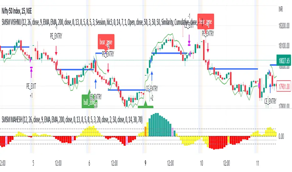
5MSM MAHESH 15It´s just the histogram of the MACD . (Actually it´s not a histogram, I like the Area visualisation more. But you can switch.)
5min stock market property
When I´m using the MACD , I´m just searching for a divergence between Price and the MACD-histogram. I´m not interested in the MACD-signalline or the MACD-line in any way. As you can see, The omission of them leads to better visualisation. It´s much easier to spot a divergence. On the one hand because that way the histogram scales bigger, on the other hand becauce the lines can´t overdraw the histogram.
Rules bullish Divergence: Price makes a lower low, oscillator makes higher low.
Rules bearish Divergence: Price makes a higher high, oscillator makes lower high.
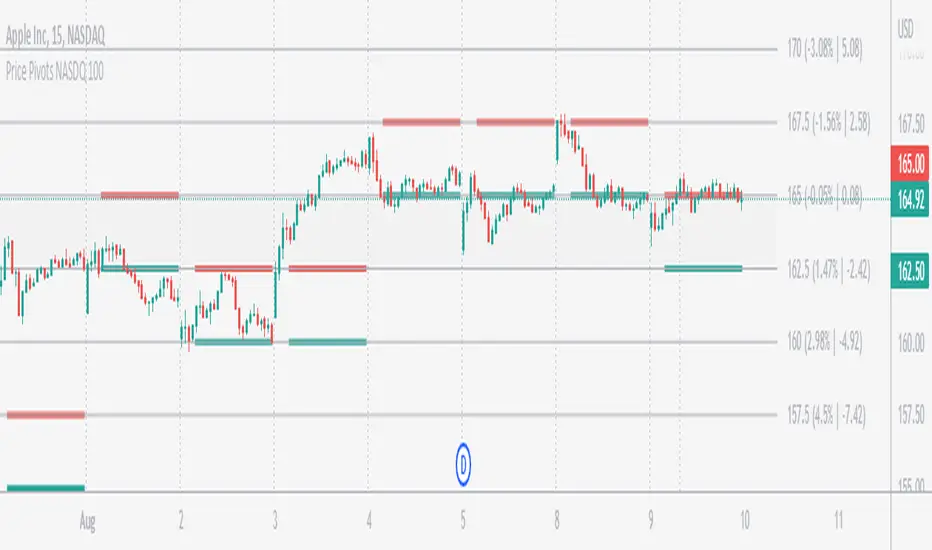
Price Pivots for NASDQ 100 StocksPrice Pivots for NASDQ 100 Stocks
What is this Indicator?
• This indicator calculates the price range a Stock can move in a Day.
Advantages of this Indicator
• This is a Leading indicator, not Dynamic or Repaint.
• Helps to identify the tight range of price movement.
• Can easily identify the Options strike price.
• Develops a discipline in placing Targets.
Disadvantages of this Indicator
• The indicator is specifically made for NASDQ 100 stocks. The levels won't work for other stocks.
• The indicator shows nothing for other indexes and stocks other than above mentioned.
• The data need to be entered manually.
Who to use?
Highly beneficial for Day Traders, it can be used for Swing and Positions as well.
What timeframe to use?
• Any timeframe.
• The highlighted levels in Red and Green will not show correct levels in 1 minute timeframe.
• 5min is recommended for Day Traders.
When to use?
• Wait for proper swing to form.
• Recommended to avoid 1st 1 hour or market open, that is 9.15am to 10.15 or 10.30am.
• Within this time a proper swing will be formed.
What are the Lines?
• The concept is the price will move from one pivot to another.
• Entry and Exit can be these levels as Reversal or Retracement.
Gray Lines:
• Every lines with price labels are the Strike Prices in the Option Chain.
• Price moves from 1 Strike Price level to another.
• The dashed lines are average levels of 2 Strike Prices.
Red & Green Lines:
• The Red and Green Lines will appear only after the first 1 hour.
• The levels are calculated based on the 1st 1 hour.
• Red Lines are important Resistance levels, these are strong Bearish reversal points. It is also a breakout level, this need to be figured out from the past levels, trend, percentage change and consolidation.
• Green Lines are important Support levels, these are strong Bullish reversal points. It is also a breakdown level, this need to be figured out from the past levels, trend, percentage change and consolidation.
What are the Labels?
• First Number: Price of that level.
• Numbers in (): Percentage change and Change of price from LTP (Last Traded Price) to that Level.
How to use?
Entry:
• Enter when price is closer to the Red or Green lines.
• Enter after considering previous Swing and Trend.
• Note the 50% of previous Swing.
• Enter Short when price reverse from each level.
• If 50% of swing and the pivot level is closer it can be a good entry.
Exit:
• Use the logic of Entry, each level can be a target.
• Exit when price is closer to the Red or Green lines.
Indicator Menu
Source
• Custom: Enter the price manually after choosing the Source as Custom to show the Pivots at that price.
• LTP: Pivot is calculated based on Last Traded Price.
• Day Open: Pivot is calculated based on current day opening price.
• PD Close: Pivot is calculated based on previous day closing price.
• PD HL2: Pivot is calculated based on previous day average of High and Low.
• PD HLC3: Pivot is calculated based on previous day average of High, Low and Close.
"Time (Vertical Lines)"
• This is a marker of every 1 hour.
• Usually major price movement happen between previous day last 1 hour to today first 1 hour.
• Two swings can happen between first 2 hour of current day.
• At the end of the day last 1 hour another important movement will happen.
• Usually rest of the time won't show any interesting movement.
To the Users
• Certain symbols may show the levels as a single line. For such symbols choose a different Source or Timeframe from the indicator menu.
• Please inform if any of the Symbol's price levels don't react to the pivots , include the Symbol a well.
• Also inform if you notice any wrong values, errors or abnormal behavior in the indicator.
• Feel free to suggest or adding new features and options.
General Tips
• It is good if Stock trend is same as that of Index trend.
• Lots of indicators creates lots of confusion.
• Keep the chart simple and clean.
• Buy Low and Sell High.
• Master averages or 50%.
• Previous Swing High and Swing Low are crucial.
Important Note
• Currently the levels are in testing stage.
• Eventually the levels of certain symbols will be corrected after each update and test.
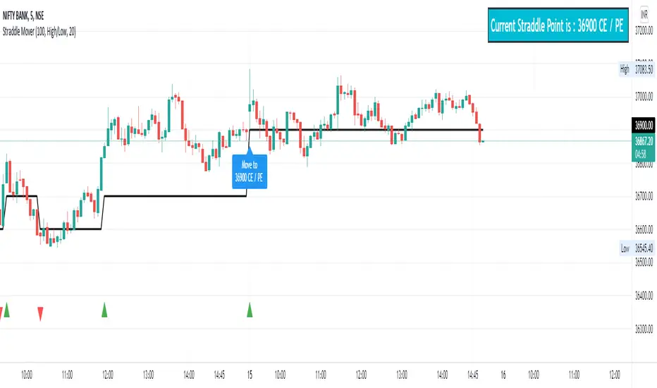
Straddle MoverStraddle Mover is an indicator especially made for option writer / seller who wants to do straddle and adjust the position based on the market trend / movement. It can be use for iron fly strategy too.
Settings: User must know the settings of the indicator before using.
First one is Option Strike Difference , user need to enter the correct option strike difference of the particular instrument / stock / indices, one can get it from option chain. For example, Nifty having 50 points differences in each option strike and bank nifty having 100 points. So, Nifty user must enter 50 and Bank nifty user must enter 100 in this setting.
Second is Straddle Type based on , user can choose the type of the straddle mover. There are two options to choose, 1) High/Low is based on current day high/low average near strike to make straddle and 2) Trend is based on recent N number of candle(s) average near strike to make straddle.
Third is Trend Length , default value is 20 which generally used in vwma , donchian channel and other trend finding indicators. User can change if need.
If user select high/low based type then length is not important.
Note : Option Strike Difference and Straddle type based on is very important setting to use this indicator.
User must do adjustments based on their own risk and strategy. This indicator is only for education purpose.
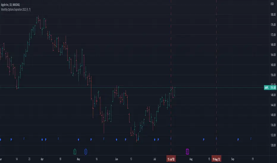
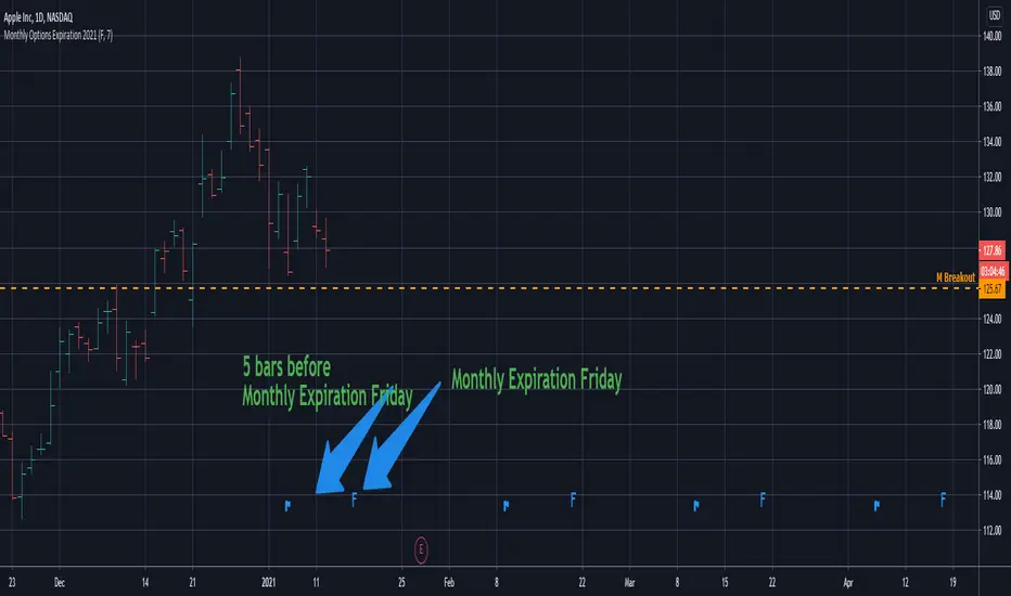
Monthly Options Expiration 2022Monthly options expiration for the year 2022.
Also you can set a flag X no. of days before the expiration date. I use it at as marker to take off existing positions in expiration week or roll to next expiration date or to place new trades.
Happy new year 2022 in advance and all the best traders.
Weekly Put SaleWeekly Put Sale
This study is a tool I use for selling weekly puts at the suggested strike prices.
1. The suggested strike prices are based on the weekly high minus an ATR multiple which can be adjusted in the settings
2. You can also adjust the settings to Monthly strike prices if you prefer selling options further out
3. I suggest looking for Put sale premium that is between 0.25% to 0.75% of the strike price for weekly Puts and 1% to 3% of the strike price for monthly Puts
Disclaimers: Selling Puts is an advanced strategy that is risky if you are not prepared to acquire the stock at the strike price you sell at on the expiration date. You must make your own decisions as you will bear the risks associated with any trades you place. To sum it up, trading is risky, and do so at your own risk.
Options Scalping V2This Indicator is Owned by Team Option Scalping.
It has 4 Plots and 2 Tables.
This indicator to be used only in BankNifty Futures
VWAP ( Volume weighted average price )
• User can input the source and enable/disable the VWAP from input section.
• When price is more than the VWAP its Bullish Trend and vice versa.
VWMA ( Volume weighted moving average )
• Default value of 20 is used in VWMA . User can enable/disable it from input section.
• When price is more than the VWMA its Bullish Trend and vice versa.
Parabolic SAR
• User can input “start”, “increment” and “maximum” values from input section and can enable/disable SAR also.
• When price is more than the Parabolic SAR its Bullish Trend and vice versa.
SuperTrend
• User can input ATR Period and ATR Multiplier values from input section. By defaults it’s 10 and 2.
• User have option of enable/disable “Change ATR calculation Method”, if enabled then ATR is calculated differently for SuperTrend.
• Enable/disable “BUY/SELL signals” on SuperTrend.
• When price is more than the SuperTrend its Bullish Trend and vice versa.
Top Right Corner TABLE ( 6 , 10 )
When you are trading in Banknifty futures , we have to check major Banks which is contributing to Banknifty move. So we have given that in this tab.
This table consist data of 9 following stocks:
• BankNifty
• Nifty
• Dow
• INDIA
• VIX
• HDFC
• ICICI
• KOTAK
• AXIS
• SBI
And following data of each stock has been provided:
• LTP
• Daily Change
• Daily Percentage Change
• 15-minute Change Percentage
• 1-Hour Change Percentage
Bottom Right Corner TABLE (3, 6 )
This table consist of 4 indicators values and Up/Down indicator:
• VWMA (When price is more than the VWMA its Bullish and vice versa)
• SuperTrend (10.2, When price is more than the SuperTrend its Bullish and vice versa.)
• RSI (14)
• VWAP (When price is more than the VWAP its Bullish and vice versa.)

Monthly Options Expiration 2021Monthly options expiration for the year 2021.
Also you can set a flag X no. of days before the expiration date. I use it at as marker to take off existing positions in expiration week or roll to next expiration date or to place new trades.
Happy new year 2021 in advance and all the best traders.
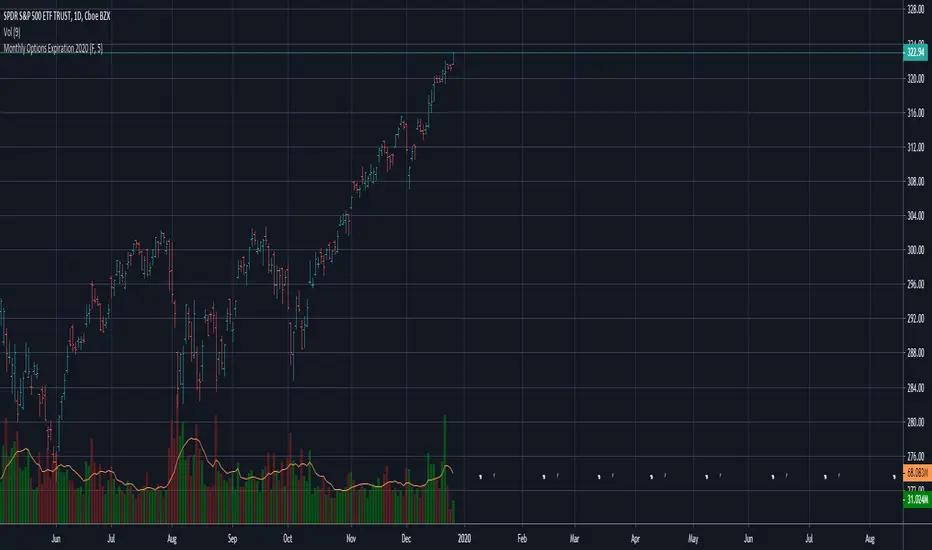
Monthly Options Expiration 2020Monthly options expiration for the year 2020.
Also you can set a flag X no. of days before the expiration date. I use it at as marker to take off existing positions in expiration week or roll to next expiration date or to place new trades.
Happy new year 2020 and all the best traders.
Monthly Options Expiration 2019All the monthly standard option expirations dates along with an option to specify a marker for X bars before. This can be used for people to mark expiration week (5 bars) or 21 days (15 bars) to expiry.
Works only on daily chart .

Apex Transformation Band EliteApex Transformation Band Elite Version
Gauge the mean range of price on an annual/yearly basis of the market.
Determine if price is in an uptrend (above the zone), neutral (inside the zone) or downtrend (below the zone).
Works on 'all' time frames.
Works for 'all' asset classes.
Customize settings for better interpretation of trend
Buy Signals (green cross)
Sell Signals (red cross)
Alert Conditions for Buy/Sell Signals
Alert Conditions for Trend change: Uptrend/Neutral/Downtrend

Apex Transformation Band ProApex Transformation Band Professional Version
Gauge the mean range of price on an annual/yearly basis of the market.
Determine if price is in an uptrend (above the zone), neutral (inside the zone) or downtrend (below the zone).
Works on 'Daily,Weekly,Monthly' time frames.
Works for all asset classes.
Feel free to ask any questions.

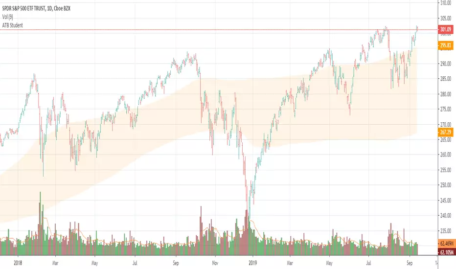
Apex Transformation Band StudentApex Transformation Band Student Version
Gauge the mean range of price on an annual/yearly basis of the market.
Determine if price is in an uptrend (above the zone), neutral (inside the zone) or downtrend (below the zone).
Works on 'Daily' time frame only.
Works only for SPY , QQQ , DIA , IWM , GLD , SLV , TLT and BTCUSD
Keep it simple.
(JS) S&P 500 Volatility Oscillator For OptionsThe idea for this started here: www.tradingview.com with the user @dime
This should only be used on SPX or SPY (though you could use it on other things for correlation I suppose) given that the instrument used to create this calculation is derived from the S&P 500 (thank you VIX). There's a lot of moving parts here though, so allow me to explain...
First: The main signal is when Implied Volatility (from VIX) drops beneath Historical Volatility - which is what you want to see so you aren't purchasing a ton of premium on long options. Green and above 0 means that IV% has dropped lower than Historical Volatility. (this signal, for example, would suggest using a Long Call or Put depending on your sentiment)
Second: The green line running underneath zero is the bottom portion of the "Average True Range" derived from the values used to create the oscillator. the closer the bottom histogram is to the green line, the more "normal" IV% is. Obviously, if this gets far away from the line then it could be setting up nicely to short options and sell the IV premium to someone else. (this signal, for example, would suggest using something like a Bull Put Spread)
Third: The red background along with the white line that drops down below zero signals when (and how far) the IV% from 3 months out (from VIX3M) is less than the current IV%. This would signal the current environment has IV way too high, a signal to short options once again (and don't take any long option positions!).
Tried to make this simple, yet effective. If you trade options on SPX, SPY, even ES1! futures - this is a tool tailored specifically for you! As I said before, if you want you can use it for correlation on other securities. Any other ideas or suggestions surrounding this, please let me know! Enjoy!
