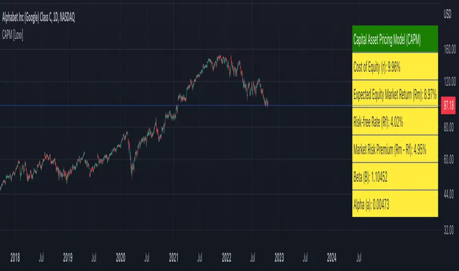
Capital Asset Pricing Model (CAPM) [Loxx]Capital Asset Pricing Model (CAPM) demonstrates how to calculate the Cost of Equity for an underlying asset using Pine Script. This script will only work on the monthly timeframe. While you can change the default inputs, you should study what CAPM is and how this works before doing so. This indicator pulls various types of data from SPY from various timeframes to calculate risk-free rates, market premiums, and log returns. Alpha and Beta are computed using the regression between underlying asset and SPY. This indicator only calculates on the most recent data. If you wish to change this, you'll have to save the script and make adjustments. A few examples where CAPM is used:
Used as the mu factor Geometric Brownian Motion models for options pricing and forecasting price ranges and decay
Calculating the Weighted Average Cost of Capital
Asset pricing
Efficient frontier
Risk and diversification
Security market line
Discounted Cashflow Analysis
Investment bankers use CAPM to value deals
Account firms use CAPM to verify asset prices and assumptions
Real estate firms use variations of CAPM to value properties
... and more
Details of the calculations used here
Rm is calculated using yearly simple returns data from SPY, typically this is just hard coded as 10%.
Rf is pulled from US 10 year bond yields
Beta and Alpha are pulled form monthly returns data of the asset and SPY
In the past, typically this data is purchased from investments banks whose research arms produce values for beta, alpha, risk free rate, and risk premiums. In 2022 ,you can find free estimates for each parameter but these values might not reflect the most current data or research.
History
The CAPM was introduced by Jack Treynor (1961, 1962), William F. Sharpe (1964), John Lintner (1965) and Jan Mossin (1966) independently, building on the earlier work of Harry Markowitz on diversification and modern portfolio theory. Sharpe, Markowitz and Merton Miller jointly received the 1990 Nobel Memorial Prize in Economics for this contribution to the field of financial economics. Fischer Black (1972) developed another version of CAPM, called Black CAPM or zero-beta CAPM, that does not assume the existence of a riskless asset. This version was more robust against empirical testing and was influential in the widespread adoption of the CAPM.
Usage
The CAPM is used to calculate the amount of return that investors need to realize to compensate for a particular level of risk. It subtracts the risk-free rate from the expected rate and weighs it with a factor – beta – to get the risk premium. It then adds the risk premium to the risk-free rate of return to get the rate of return an investor expects as compensation for the risk. The CAPM formula is expressed as follows:
r = Rf + beta (Rm – Rf) + Alpha
Therefore,
Alpha = R – Rf – beta (Rm-Rf)
Where:
R represents the portfolio return
Rf represents the risk-free rate of return
Beta represents the systematic risk of a portfolio
Rm represents the market return, per a benchmark
For example, assuming that the actual return of the fund is 30, the risk-free rate is 8%, beta is 1.1, and the benchmark index return is 20%, alpha is calculated as:
Alpha = (0.30-0.08) – 1.1 (0.20-0.08) = 0.088 or 8.8%
The result shows that the investment in this example outperformed the benchmark index by 8.8%.
The alpha of a portfolio is the excess return it produces compared to a benchmark index. Investors in mutual funds or ETFs often look for a fund with a high alpha in hopes of getting a superior return on investment (ROI).
The alpha ratio is often used along with the beta coefficient, which is a measure of the volatility of an investment. The two ratios are both used in the Capital Assets Pricing Model (CAPM) to analyze a portfolio of investments and assess its theoretical performance.
To see CAPM in action in terms of calculate WACC, see here for an example: finbox.com
Further reading
en.wikipedia.org
Search in scripts for "1990年+黄金价格+历史数据"
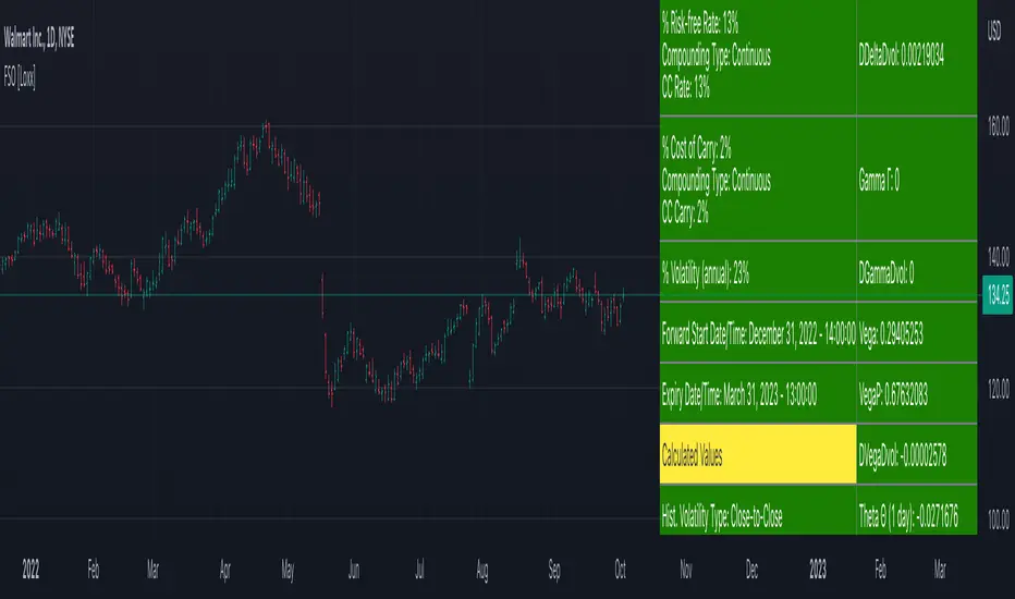
Forward Start Options [Loxx]A forward start option with time to maturity T starts at-the-money or proportionally in- or out-of-the-money after a known elapsed time t in the future. The strike is set equal to a positive constant a times the asset price S after the known time t. If a is less than unity, the call (put) will start 1 - a percent in-the-money (out-of-the- money); if a is unity, the option will start at-the-money; and if a is larger than unity, the call (put) will start a - 1 percentage out-of-the- money (in-the-money).A forward start option can be priced using the Rubinstein (1990) formula: (via "The Complete Guide to Option Pricing Formulas")
c = S*e^(b-r)t * (e^(b-r)(T-t) * N(d1)) - alpha * e^-r(T-t) * N(d2))
p = S*e^(b-r)t * (alpha*e^r(T-t) * N(-d2)) - e^-(b-r)(T-t) * N(-d1))
where
d1 = (log(1/alpha) + (b + v^2/2)(T-1))/v*(T-t)^0.5
d2 = d1 - v*(T-t)^0.5
Application
Employee options are often of the forward starting type. Ratchet options (aka cliquet options) consist of a series of forward starting options.
b=r options on non-dividend paying stock
b=r-q options on stock or index paying a dividend yield of q
b=0 options on futures
b=r-rf currency options (where rf is the rate in the second currency)
Inputs
S = Stock price.
a = Alpha
T1 = Time to forward start
T = Time to expiration in years.
r = Risk-free rate
c = Cost of Carry
v = volatility of the underlying asset price
Numerical Greeks or Greeks by Finite Difference
Analytical Greeks are the standard approach to estimating Delta, Gamma etc... That is what we typically use when we can derive from closed form solutions. Normally, these are well-defined and available in text books. Previously, we relied on closed form solutions for the call or put formulae differentiated with respect to the Black Scholes parameters. When Greeks formulae are difficult to develop or tease out, we can alternatively employ numerical Greeks - sometimes referred to finite difference approximations. A key advantage of numerical Greeks relates to their estimation independent of deriving mathematical Greeks. This could be important when we examine American options where there may not technically exist an exact closed form solution that is straightforward to work with. (via VinegarHill FinanceLabs)
Things to know
Only works on the daily timeframe and for the current source price.
You can adjust the text size to fit the screen
McGinley Dynamic (Improved) - John R. McGinley, Jr.For all the McGinley enthusiasts out there, this is my improved version of the "McGinley Dynamic", originally formulated and publicized in 1990 by John R. McGinley, Jr. Prior to this release, I recently had an encounter with a member request regarding the reliability and stability of the general algorithm. Years ago, I attempted to discover the root of it's inconsistency, but success was not possible until now. Being no stranger to a good old fashioned computational crisis, I revisited it with considerable contemplation.
I discovered a lack of constraints in the formulation that either caused the algorithm to implode to near zero and zero OR it could explosively enlarge to near infinite values during unusual price action volatility conditions, occurring on different time frames. A numeric E-notation in a moving average doesn't mean a stock just shot up in excess of a few quintillion in value from just "10ish" moments ago. Anyone experienced with the usual McGinley Dynamic, has probably encountered this with dynamically dramatic surprises in their chart, destroying it's usability.
Well, I believe I have found an answer to this dilemma of 'susceptibility to miscalculation', to provide what is most likely McGinley's whole hearted intention. It required upgrading the formulation with two constraints applied to it using min/max() functions. Let me explain why below.
When using base numbers with an exponent to the power of four, some miniature numbers smaller than one can numerically collapse to near 0 values, or even 0.0 itself. A denominator of zero will always give any computational device a horribly bad day, not to mention the developer. Let this be an EASY lesson in computational division, I often entertainingly express to others. You have heard the terminology "$#|T happens!🙂" right? In the programming realm, "AnyNumber/0.0 CAN happen!🤪" too, and it happens "A LOT" unexpectedly, even when it's highly improbable. On the other hand, numbers a bit larger than 2 with the power of four can tremendously expand rapidly to the numeric limits of 64-bit processing, generating ginormous spikes on a chart.
The ephemeral presence of one OR both of those potentials now has a combined satisfactory remedy, AND you as TV members now have it, endowed with the ever evolving "Power of Pine". Oh yeah, this one plots from bar_index==0 too. It also has experimental settings tweaks to play with, that may reveal untapped potential of this formulation. This function now has gain of function capabilities, NOT to be confused with viral gain of function enhancements from reckless BSL-4 leaking laboratories that need to be eternally abolished from this planet. Although, I do have hopes this imd() function has the potential to go viral. I believe this improved function may have utility in the future by developers of the TradingView community. You have the source, and use it wisely...
I included an generic ema() plot for a basic comparison, ultimately unveiling some of this algorithm's unique characteristics differing on a variety of time frames. Also another unconstrained function is included to display some the disparities of having no limitations on a divisor in the calculation. I strongly advise against the use of umd() in any published script. There is simply just no reason to even ponder using it. I also included notes in the script to warn against this. It's funny now, but some folks don't always read/understand my advisories... You have been warned!
NOTICE: You have absolute freedom to use this source code any way you see fit within your new Pine projects, and that includes TV themselves. You don't have to ask for my permission to reuse this improved function in your published scripts, simply because I have better things to do than answer requests for the reuse of this simplistic imd() function. Sufficient accreditation regarding this script and compliance with "TV's House Rules" regarding code reuse, is as easy as copying the entire function as is. Fair enough? Good! I have a backlog of "computational crises" to contend with, including another one during the writing of this elaborate description.
When available time provides itself, I will consider your inquiries, thoughts, and concepts presented below in the comments section, should you have any questions or comments regarding this indicator. When my indicators achieve more prevalent use by TV members, I may implement more ideas when they present themselves as worthy additions. Have a profitable future everyone!

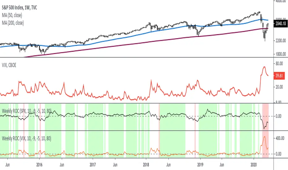
Rate Of Change - Weekly SignalsRate of Change - Weekly Signals
This indicator gives a potential "buy signal" using Rate of Change of SPX and VIX together,
using the following criteria:
SPX Weekly ROC(10) has been BELOW -9 and now rises ABOVE -5
*PLUS*
VIX Weekly ROC(10) has been ABOVE +80 and now falls BELOW +10
The background will turn RED when ROC(SPX) is below -9 and ROC(VIX) is above +80.
The background will turn GREEN when ROC(SPX) is above -5 and ROC(VIX) is below +10.
So the potential "buy signal" is when you start to get GREEN BARS AFTER RED - usually with
some white/empty bars in between...but wait for the green. This indicates that the volatility
has settled down, and the market is starting to turn up.
This indicator gives excellent entry points, but be careful of the occasional false signals.
See Nov. 2001 and Nov. 2008, in both cases the market dropped another 25-30% before the final
bottom was formed. Always have an exit strategy, especially when buying in after a downtrend.
How I use this indicator, pretty much as shown in the preview. Weekly SPX as the main chart with
some medium/long moving averages to identify the trend, VIX added as a "Compare Symbol" in red,
and then the Weekly ROC signals below.
For the ROC graphs, you can show SPX+VIX together, SPX alone, or VIX alone. I prefer to display
them separately because they don't scale well together (VIX crowds out the SPX when it spikes).
Background color is still based on both SPX/VIX together, regardless of which graph is shown.
Note that there is no VIX data available on Trading View prior to 1990, so for those dates the
formula is using only ROC(SPX) and the assigned thresholds (-9 and -5, or whatever you choose).
T7 JNSARJNSAR stands for Just Nifty -0.14% Stop & Reverse. This is a Trend Following Daily Bar Trading System for NIFTY -0.14% . Original idea belongs to ILLANGO @ I coded the pine version of this system based on a request from @stocksonfire. Use it at your own risk after validation at your end. Neither me or my company is responsible for any losses you may incur using this system. Hope you like this system and enjoy trading it !!!
Updated V3 code for the T7 JNSAR system earlier published here V2 and here V1
Following updates made to the code
1. Added a 22 Period Simple moving average filter over and above the standard JNSAR value for generating trading signals. This simple filter reduces the whipsaw trades drastically along with similar improvements in the max draw down and overall profitability of the system. The SMA filter is turned ON by default but can be turned OFF by user through the settings window.
2. Backtest option is now turned ON by default.
Also am republishing the trading rules here again with some modification
1. Go Long when the daily close is above the JNSAR line. Go Short when the daily close is below the JNSAR line. JNSAR line is the varying green line overlayed over the price chart. Once a signal comes at market close enter in the direction of the signal @ market price @ next day market open.
2. Trade only Nifty -0.14% Index. This system was developed and backtested only for NIFTY -0.14% Index. So trade in its Futures or Options, as you may deem fit. My recommendation is to choose futures for simplicity. If you want to reduce the trading cost and go with options, trade with deep in the money options, preferably 2 strikes far from the spot price.
3. Trade all signals. Markets trend only 30-35% of the time and hence the system is only accurate to that extend. But system tends to make enough money, in this small trending window, to keep the overall profitability in good health. But one never knows when a big trend may come and when it comes its absolutely imperative that you take it. To ensure that, trade all signals and don't be choosy about what signals you are going to trade. Also I wouldn't recommend using your own analysis to trade this system. Too many drivers will crash the car.
4. Like all trend following systems, this system will have many whipsaws during flat markets along with large trade and account drawdowns. Also some months and even years may not be profitable. But to trade this system profitably, it is necessary to take these in one's stride and keep trading. As the backtester results from 1990 to 2017 proves, this system is profitable overall thus far. Take confidence from that objective fact.
5. Trade with only that amount of money you can afford to loose. Initial capital that you need to have to trade one lot of NIFTY -0.14% should be atleast - (Margin Money required to take and hold 1 lot position + maximum drawdown amount per lot)*1.2. Be prepared to add more if need be, but the above formula will give a rough idea of what you need to have to start trading and be in the game always.
6. Place an After Market Order @ Market Price with your broker after market close so that you get to execute the trade next trading day @ Market open to capture near similar price as the daily open price seen on the chart. This execution mode will give you the best chance to minimize the slippage and mimic the backtester results as closely as practically possible.
7. Follow all the 6 rules above religiously, as if your life depends on it. If you cant, then don't trade this system; You will certainly loose money.
Happy Trading !!! As always am looking out for your valuable feedback.

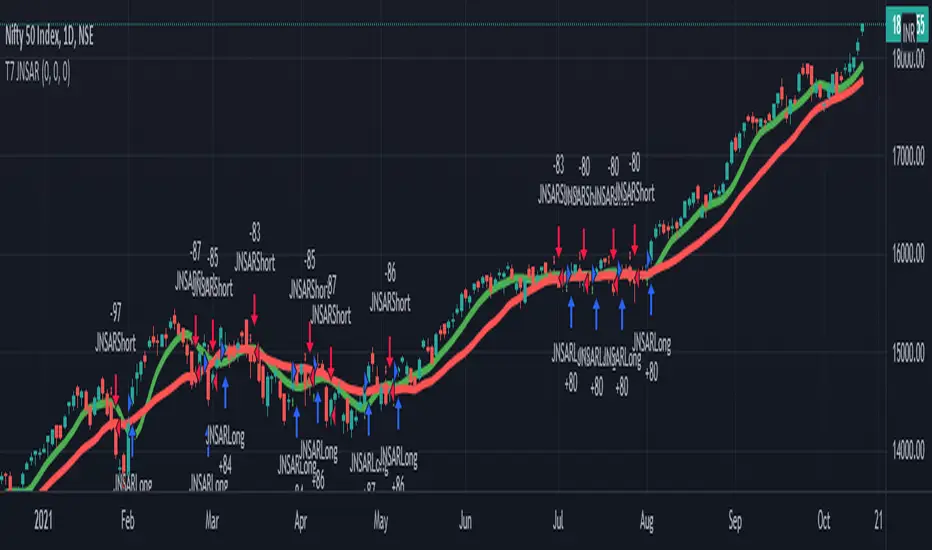
T7 JNSARUpdated code for the T7 JNSAR system earlier published here -
Following updates made to the code
1. Buy / Sell arrows now appear when the corresponding conditions are met.
2. Support for Heikin-Ashi Candles added
3. Different Backtesting Position Sizing Algorithms added for evaluation
Also am republishing the trading rules here again with some modification
1. Go Long when the daily close is above the JNSAR line. Go Short when the daily close is below the JNSAR line. JNSAR line is the varying green line overlayed over the price chart. Once a signal comes at market close enter in the direction of the signal @ market price @ next day market open.
2. Trade only Nifty Index. This system was developed and backtested only for NIFTY Index. So trade in its Futures or Options, as you may deem fit. My recommendation is to choose futures for simplicity. If you want to reduce the trading cost and go with options, trade with deep in the money options, preferably 2 strikes far from the spot price.
3. Trade all signals. Markets trend only 30-35% of the time and hence the system is only accurate to that extend. But system tends to make enough money, in this small trending window, to keep the overall profitability in good health. But one never knows when a big trend may come and when it comes its absolutely imperative that you take it. To ensure that, trade all signals and don't be choosy about what signals you are going to trade. Also I wouldn't recommend using your own analysis to trade this system. Too many drivers will crash the car.
4. Like all trend following systems, this system will have many whipsaws during flat markets along with large trade and account drawdowns. Also some months and even years may not be profitable. But to trade this system profitably, it is necessary to take these in one's stride and keep trading. As the backtester results from 1990 to 2016 proves, this system is profitable overall thus far. Take confidence from that objective fact.
5. Trade with only that amount of money you can afford to loose. Initial capital that you need to have to trade one lot of NIFTY should be atleast - (Margin Money required to take and hold 1 lot position + maximum drawdown amount per lot)*1.2. Be prepared to add more if need be, but the above formula will give a rough idea of what you need to have to start trading and be in the game always.
6. Place an After Market Order @ Market Price with your broker after market close so that you get to execute the trade next trading day @ Market open to capture near similar price as the daily open price seen on the chart. This execution mode will give you the best chance to minimise the slippage and mimic the backtester results as closely as practically possible.
7. Follow all the 6 rules above religiously, as if your life depends on it. If you cant, then don't trade this system; You will certainly loose money.
Happy Trading !!! As always am looking out for your valuable feedback.
T7 JNSARJNSAR stands for Just Nifty Stop & Reverse. This is a trend following daily bar trading system for NIFTY. Original idea belongs to ILLANGO @ I coded the pine version of this system based on a request from @stocksonfire. Use it at your own risk after validation at your end. Neither me or my company is responsible for any losses you may incur using this system. Hope you like this system and enjoy trading it !!!
While trading this system you must follow these simple rules.
1. Go Long when the daily close is above the JNSAR line. Go Short when the daily close is below the JNSAR line. JNSAR line is the varying green line overlayed over the price chart. Once a signal comes at market close enter in the direction of the signal @ market price @ next day market open.
2. Trade only Nifty Index. This system was developed and backtested only for NIFTY Index. So trade in its Futures or Options, as you may deem fit. My recommendation is to choose futures for simplicity. If you want to reduce the trading cost and go with options, trade with deep in the money options, preferably 2 strikes far from the spot price.
3. Trade all signals. Markets trend only 30-35% of the time and hence the system is only accurate to that extend. But system tends to make enough money, in this small trending window, to keep the overall profitability in good health. But one never knows when a big trend may come and when it comes its absolutely imperative that you take it. To ensure that, trade all signals and don't be choosy about what signals you are going to trade. Also I wouldn't recommend using your own analysis to trade this system. Too many drivers will crash the car.
4. Like all trend following systems, this system will have many whipsaws during flat markets along with large trade and account drawdowns. Also some months and even years may not be profitable. But to trade this system profitably, it is necessary to take these in one's stride and keep trading. As the backtester results from 1990 to 2016 proves, this system is profitable overall thus far. Take confidence from that objective fact.
5. Initial capital that you need to have to trade one lot of NIFTY should be atleast - (Margin Money required to take and hold 1 lot position + maximum drawdown amount per lot)*1.2. Be prepared to add more if need be, but the above formula will give a rough idea of what you need to have to start trading and be in the game always.
6. Follow all the 5 rules above religiously as if your life depends on it. If you cant, then don't trade this system; You will certainly loose money.