Advanced Petroleum Market Model (APMM)Advanced Petroleum Market Model (APMM): A Multi-Factor Fundamental Analysis Framework for Oil Market Assessment
## 1. Introduction
The petroleum market represents one of the most complex and globally significant commodity markets, characterized by intricate supply-demand dynamics, geopolitical influences, and substantial price volatility (Hamilton, 2009). Traditional fundamental analysis approaches often struggle to synthesize the multitude of relevant indicators into actionable insights due to data heterogeneity, temporal misalignment, and subjective weighting schemes (Baumeister & Kilian, 2016).
The Advanced Petroleum Market Model addresses these limitations through a systematic, quantitative approach that integrates 16 verified fundamental indicators across five critical market dimensions. The model builds upon established financial engineering principles while incorporating petroleum-specific market dynamics and adaptive learning mechanisms.
## 2. Theoretical Framework
### 2.1 Market Efficiency and Information Integration
The model operates under the assumption of semi-strong market efficiency, where fundamental information is gradually incorporated into prices with varying degrees of lag (Fama, 1970). The petroleum market's unique characteristics, including storage costs, transportation constraints, and geopolitical risk premiums, create opportunities for fundamental analysis to provide predictive value (Kilian, 2009).
### 2.2 Multi-Factor Asset Pricing Theory
Drawing from Ross's (1976) Arbitrage Pricing Theory, the model treats petroleum prices as driven by multiple systematic risk factors. The five-factor decomposition (Supply, Inventory, Demand, Trade, Sentiment) represents economically meaningful sources of systematic risk in petroleum markets (Chen et al., 1986).
## 3. Methodology
### 3.1 Data Sources and Quality Framework
The model integrates 16 fundamental indicators sourced from verified TradingView economic data feeds:
Supply Indicators:
- US Oil Production (ECONOMICS:USCOP)
- US Oil Rigs Count (ECONOMICS:USCOR)
- API Crude Runs (ECONOMICS:USACR)
Inventory Indicators:
- US Crude Stock Changes (ECONOMICS:USCOSC)
- Cushing Stocks (ECONOMICS:USCCOS)
- API Crude Stocks (ECONOMICS:USCSC)
- API Gasoline Stocks (ECONOMICS:USGS)
- API Distillate Stocks (ECONOMICS:USDS)
Demand Indicators:
- Refinery Crude Runs (ECONOMICS:USRCR)
- Gasoline Production (ECONOMICS:USGPRO)
- Distillate Production (ECONOMICS:USDFP)
- Industrial Production Index (FRED:INDPRO)
Trade Indicators:
- US Crude Imports (ECONOMICS:USCOI)
- US Oil Exports (ECONOMICS:USOE)
- API Crude Imports (ECONOMICS:USCI)
- Dollar Index (TVC:DXY)
Sentiment Indicators:
- Oil Volatility Index (CBOE:OVX)
### 3.2 Data Quality Monitoring System
Following best practices in quantitative finance (Lopez de Prado, 2018), the model implements comprehensive data quality monitoring:
Data Quality Score = Σ(Individual Indicator Validity) / Total Indicators
Where validity is determined by:
- Non-null data availability
- Positive value validation
- Temporal consistency checks
### 3.3 Statistical Normalization Framework
#### 3.3.1 Z-Score Normalization
The model employs robust Z-score normalization as established by Sharpe (1994) for cross-indicator comparability:
Z_i,t = (X_i,t - μ_i) / σ_i
Where:
- X_i,t = Raw value of indicator i at time t
- μ_i = Sample mean of indicator i
- σ_i = Sample standard deviation of indicator i
Z-scores are capped at ±3 to mitigate outlier influence (Tukey, 1977).
#### 3.3.2 Percentile Rank Transformation
For intuitive interpretation, Z-scores are converted to percentile ranks following the methodology of Conover (1999):
Percentile_Rank = (Number of values < current_value) / Total_observations × 100
### 3.4 Exponential Smoothing Framework
Signal smoothing employs exponential weighted moving averages (Brown, 1963) with adaptive alpha parameter:
S_t = α × X_t + (1-α) × S_{t-1}
Where α = 2/(N+1) and N represents the smoothing period.
### 3.5 Dynamic Threshold Optimization
The model implements adaptive thresholds using Bollinger Band methodology (Bollinger, 1992):
Dynamic_Threshold = μ ± (k × σ)
Where k is the threshold multiplier adjusted for market volatility regime.
### 3.6 Composite Score Calculation
The fundamental score integrates component scores through weighted averaging:
Fundamental_Score = Σ(w_i × Score_i × Quality_i)
Where:
- w_i = Normalized component weight
- Score_i = Component fundamental score
- Quality_i = Data quality adjustment factor
## 4. Implementation Architecture
### 4.1 Adaptive Parameter Framework
The model incorporates regime-specific adjustments based on market volatility:
Volatility_Regime = σ_price / μ_price × 100
High volatility regimes (>25%) trigger enhanced weighting for inventory and sentiment components, reflecting increased market sensitivity to supply disruptions and psychological factors.
### 4.2 Data Synchronization Protocol
Given varying publication frequencies (daily, weekly, monthly), the model employs forward-fill synchronization to maintain temporal alignment across all indicators.
### 4.3 Quality-Adjusted Scoring
Component scores are adjusted for data quality to prevent degraded inputs from contaminating the composite signal:
Adjusted_Score = Raw_Score × Quality_Factor + 50 × (1 - Quality_Factor)
This formulation ensures that poor-quality data reverts toward neutral (50) rather than contributing noise.
## 5. Usage Guidelines and Best Practices
### 5.1 Configuration Recommendations
For Short-term Analysis (1-4 weeks):
- Lookback Period: 26 weeks
- Smoothing Length: 3-5 periods
- Confidence Period: 13 weeks
- Increase inventory and sentiment weights
For Medium-term Analysis (1-3 months):
- Lookback Period: 52 weeks
- Smoothing Length: 5-8 periods
- Confidence Period: 26 weeks
- Balanced component weights
For Long-term Analysis (3+ months):
- Lookback Period: 104 weeks
- Smoothing Length: 8-12 periods
- Confidence Period: 52 weeks
- Increase supply and demand weights
### 5.2 Signal Interpretation Framework
Bullish Signals (Score > 70):
- Fundamental conditions favor price appreciation
- Consider long positions or reduced short exposure
- Monitor for trend confirmation across multiple timeframes
Bearish Signals (Score < 30):
- Fundamental conditions suggest price weakness
- Consider short positions or reduced long exposure
- Evaluate downside protection strategies
Neutral Range (30-70):
- Mixed fundamental environment
- Favor range-bound or volatility strategies
- Wait for clearer directional signals
### 5.3 Risk Management Considerations
1. Data Quality Monitoring: Continuously monitor the data quality dashboard. Scores below 75% warrant increased caution.
2. Regime Awareness: Adjust position sizing based on volatility regime indicators. High volatility periods require reduced exposure.
3. Correlation Analysis: Monitor correlation with crude oil prices to validate model effectiveness.
4. Fundamental-Technical Divergence: Pay attention when fundamental signals diverge from technical indicators, as this may signal regime changes.
### 5.4 Alert System Optimization
Configure alerts conservatively to avoid false signals:
- Set alert threshold at 75+ for high-confidence signals
- Enable data quality warnings to maintain system integrity
- Use trend reversal alerts for early regime change detection
## 6. Model Validation and Performance Metrics
### 6.1 Statistical Validation
The model's statistical robustness is ensured through:
- Out-of-sample testing protocols
- Rolling window validation
- Bootstrap confidence intervals
- Regime-specific performance analysis
### 6.2 Economic Validation
Fundamental accuracy is validated against:
- Energy Information Administration (EIA) official reports
- International Energy Agency (IEA) market assessments
- Commercial inventory data verification
## 7. Limitations and Considerations
### 7.1 Model Limitations
1. Data Dependency: Model performance is contingent on data availability and quality from external sources.
2. US Market Focus: Primary data sources are US-centric, potentially limiting global applicability.
3. Lag Effects: Some fundamental indicators exhibit publication lags that may delay signal generation.
4. Regime Shifts: Structural market changes may require model recalibration.
### 7.2 Market Environment Considerations
The model is optimized for normal market conditions. During extreme events (e.g., geopolitical crises, pandemics), additional qualitative factors should be considered alongside quantitative signals.
## References
Baumeister, C., & Kilian, L. (2016). Forty years of oil price fluctuations: Why the price of oil may still surprise us. *Journal of Economic Perspectives*, 30(1), 139-160.
Bollinger, J. (1992). *Bollinger on Bollinger Bands*. McGraw-Hill.
Brown, R. G. (1963). *Smoothing, Forecasting and Prediction of Discrete Time Series*. Prentice-Hall.
Chen, N. F., Roll, R., & Ross, S. A. (1986). Economic forces and the stock market. *Journal of Business*, 59(3), 383-403.
Conover, W. J. (1999). *Practical Nonparametric Statistics* (3rd ed.). John Wiley & Sons.
Fama, E. F. (1970). Efficient capital markets: A review of theory and empirical work. *Journal of Finance*, 25(2), 383-417.
Hamilton, J. D. (2009). Understanding crude oil prices. *Energy Journal*, 30(2), 179-206.
Kilian, L. (2009). Not all oil price shocks are alike: Disentangling demand and supply shocks in the crude oil market. *American Economic Review*, 99(3), 1053-1069.
Lopez de Prado, M. (2018). *Advances in Financial Machine Learning*. John Wiley & Sons.
Ross, S. A. (1976). The arbitrage theory of capital asset pricing. *Journal of Economic Theory*, 13(3), 341-360.
Sharpe, W. F. (1994). The Sharpe ratio. *Journal of Portfolio Management*, 21(1), 49-58.
Tukey, J. W. (1977). *Exploratory Data Analysis*. Addison-Wesley.
Search in scripts for "30年国债收益率"

RSI Multi-TF TabRSI Multi-Timeframe Table 📊
A tool for multi-timeframe RSI analysis with visual overbought/oversold level highlighting.
Description
This indicator calculates the Relative Strength Index (RSI) for the current chart and displays RSI values across five additional timeframes (15m, 1h, 4h, 1d, 1w) in a dynamic table. The color-coded system simplifies identifying overbought (>70), oversold (<30), and neutral zones. Visual signals on the chart enhance analysis for the current timeframe.
Key Features
✅ Multi-Timeframe Analysis :
Track RSI across 15m, 1h, 4h, 1d, and 1w in a compact table.
Color-coded alerts:
🔴 Red — Overbought (potential pullback),
🔵 Blue — Oversold (potential rebound),
🟡 Yellow — Neutral zone.
✅ Visual Signals :
Background shading for oversold/overbought zones on the main chart.
Horizontal lines at 30 and 70 levels for reference.
✅ Customizable Settings :
Adjust RSI length (default: 14), source (close, open, high, etc.), and threshold levels.
How to Use
Table Analysis :
Compare RSI values across timeframes to spot divergences (e.g., overbought on 15m vs. oversold on D).
Use colors for quick decisions.
Chart Signals :
Blue background suggests bullish potential (oversold), red hints at bearish pressure (overbought).
Always confirm with other tools (volume, trends, or candlestick patterns).
Examples :
RSI(1h) > 70 while RSI(4h) < 30 → Possible reversal upward.
Sustained RSI(1d) above 50 may indicate a bullish trend.
Settings
RSI Length : Period for RSI calculation (default: 14).
RSI Source : Data source (close, open, high, low, hl2, hlc3, ohlc4).
Overbought/Oversold Levels : Thresholds for alerts (default: 70/30).
Important Notes
No direct trading signals : Use this as an analytical tool, not a standalone strategy.
Test strategies historically and consider market context before trading.

Canuck Trading Projection IndicatorCanuck Trading Projection Indicator
Overview
The Canuck Trading Projection Indicator is a powerful PineScript v6 tool designed for TradingView to project potential bullish and bearish price trajectories based on historical price and volume movements. It provides traders with actionable insights by estimating future price targets and assigning confidence levels to each outlook, helping to identify probable market directions across any timeframe. Ideal for both short-term and long-term traders, this indicator combines momentum analysis, RSI filtering, support/resistance detection, and time-weighted trend analysis to deliver robust projections.
Features
Bullish and Bearish Projections: Forecasts price targets for upward (bullish) and downward (bearish) movements over a user-defined projection period (default 20 bars).
Confidence Levels: Assigns percentage confidence scores to each outlook, reflecting the likelihood of the projected price based on historical trends, volatility, and volume.
RSI Filter: Incorporates a 14-period Relative Strength Index (RSI) to validate trends, requiring RSI > 50 for bullish and RSI < 50 for bearish signals.
Support/Resistance Detection: Adjusts confidence levels when projections are near key swing highs/lows (within 2% of average price), boosting confidence by 5% for alignments.
Time-Based Weighting: Prioritizes recent price movements in trend analysis, giving more weight to newer bars for improved relevance.
Customizable Inputs: Allows users to tailor lookback period, projection bars, RSI period, confidence threshold, colors, and label positioning.
Forced Label Spacing: Prevents overlap of bullish and bearish text labels, even for tight projections, using fixed vertical slots when price differences are small (<2% of average price).
Timeframe Flexibility: Works seamlessly across all TradingView timeframes (e.g., 30-minute, hourly, daily, weekly, monthly), adapting projections to the chart’s resolution.
Clean Visualization: Displays projections as green (bullish) and red (bearish) dashed lines, with non-overlapping text labels at the projection endpoints showing price targets and confidence levels.
How It Works
The indicator analyzes historical price and volume data over a user-defined lookback period (default 50 bars) to calculate:
Momentum: Combines price changes and volume to assess trend strength, using a weighted moving average (WMA) for directional bias.
Trend Analysis: Counts bullish (price up, volume above average, RSI > 50) and bearish (price down, volume above average, RSI < 50) trends, weighting recent bars more heavily.
Projections:
Bullish Slope: Positive or flat when momentum is upward, scaled by price change and momentum intensity.
Bearish Slope: Negative or flat when momentum is downward, amplified by bearish confidence for stronger projections.
Projects prices forward by 20 bars (default) using current close plus slope times projection bars.
Confidence Levels:
Base confidence derived from the proportion of bullish/bearish trends, with a 5% minimum to avoid zero confidence.
Adjusted by volatility (lower volatility increases confidence), volume trends, and proximity to support/resistance levels.
Visualization:
Draws projection lines from the current close to the 20-bar future target.
Places text labels at line endpoints, showing price targets and confidence percentages, with forced spacing for readability.
Input Parameters
Lookback Period (default: 50): Number of bars for historical analysis (minimum 10).
Projection Bars (default: 20): Number of bars to project forward (minimum 5).
Confidence Threshold (default: 0.6): Minimum confidence for strong trend indication (0.1 to 1.0).
Bullish Projection Line Color (default: Green): Color for bullish projection line and label.
Bearish Projection Line Color (default: Red): Color for bearish projection line and label.
RSI Period (default: 14): Period for RSI momentum filter (minimum 5).
Label Vertical Offset (%) (default: 1.0): Base offset for labels as a percentage of price range (0.1% to 5.0%).
Minimum Label Spacing (%) (default: 2.0): Minimum vertical spacing between labels for tight projections (0.5% to 10.0%).
Usage Instructions
Add to Chart: Copy the script into TradingView’s Pine Editor, save, and add the indicator to your chart.
Select Timeframe: Apply to any timeframe (e.g., 30-minute, hourly, daily, weekly, monthly) to match your trading strategy.
Interpret Outputs:
Green Line/Label: Bullish price target and confidence (e.g., "Bullish: 414.37, Confidence: 35%").
Red Line/Label: Bearish price target and confidence (e.g., "Bearish: 279.08, Confidence: 41.3%").
Higher confidence indicates a stronger likelihood of the projected outcome.
Adjust Inputs:
Modify Lookback Period to focus on shorter/longer historical trends (e.g., 20 for short-term, 100 for long-term).
Change Projection Bars to adjust forecast horizon (e.g., 10 for shorter, 50 for longer).
Tweak RSI Period or Confidence Threshold for sensitivity to momentum or trend strength.
Customize Colors for visual preference.
Increase Minimum Label Spacing if labels overlap in volatile markets.
Combine with Analysis: Use alongside other indicators (e.g., moving averages, Bollinger Bands) or fundamental analysis to confirm signals, as projections are probabilistic.
Example: TSLA Across Timeframes
Using live TSLA data (close ~346.46 USD, May 31, 2025), the indicator produces:
30-Minute: Bullish 341.93 (13.3%), Bearish 327.96 (86.7%) – Strong bearish sentiment due to intraday volatility.
1-Hour: Bullish 342.00 (33.9%), Bearish 327.50 (62.3%) – Bearish but less intense, reflecting hourly swings.
4-Hour: Bullish 345.52 (73.4%), Bearish 344.44 (19.0%) – Flat outlook, indicating consolidation.
Daily: Bullish 391.26 (68.8%), Bearish 302.22 (31.2%) – Bullish bias from recent uptrend, bearish tempered by longer lookback.
Weekly: Bullish 414.37 (35.0%), Bearish 279.08 (41.3%) – Wide range, reflecting annual volatility.
Monthly: Bullish 396.70 (54.9%), Bearish 296.93 (10.2%) – Long-term bullish optimism.
These results align with market dynamics: short-term intervals capture volatility, while longer intervals smooth trends, providing balanced outlooks.
Notes
Accuracy: Projections are estimates based on historical data and should be used with other analysis tools. Confidence levels indicate likelihood, not certainty.
Timeframe Sensitivity: Short-term intervals (e.g., 30-minute) show larger price swings and higher confidence due to volatility, while longer intervals (e.g., monthly) are more stable.
Customization: Adjust inputs to match your trading style (e.g., shorter lookback for day trading, longer for swing trading).
Performance: Tested on volatile stocks like TSLA, NVIDIA, and others, ensuring robust performance across markets.
Limitations: May produce conservative bearish projections in strong uptrends due to momentum weighting. Adjust lookback or projection_bars for sensitivity.
Feedback
If you encounter issues (e.g., label overlap, projection mismatches), please share your timeframe, settings, or a screenshot. Suggestions for enhancements (e.g., additional filters, visual tweaks) are welcome!
Disclaimer
The Canuck Trading Projection Indicator is provided for educational and informational purposes only. It is not financial advice. Trading involves significant risks, and past performance is not indicative of future results. Always perform your own due diligence and consult a qualified financial advisor before making trading decisions.

MACD + RSI + EMA + BB + ATR Day Trading StrategyEntry Conditions and Signals
The strategy implements a multi-layered filtering approach to entry conditions, requiring alignment across technical indicators, timeframes, and market conditions .
Long Entry Requirements
Trend Filter: Fast EMA (9) must be above Slow EMA (21), price must be above Fast EMA, and higher timeframe must confirm uptrend
MACD Signal: MACD line crosses above signal line, indicating increasing bullish momentum
RSI Condition: RSI below 70 (not overbought) but above 40 (showing momentum)
Volume & Volatility: Current volume exceeds 1.2x 20-period average and ATR shows sufficient market movement
Time Filter: Trading occurs during optimal hours (9:30-11:30 AM ET) when market volatility is typically highest
Exit Strategies
The strategy employs multiple exit mechanisms to adapt to changing market conditions and protect profits :
Stop Loss Management
Initial Stop: Placed at 2.0x ATR from entry price, adapting to current market volatility
Trailing Stop: 1.5x ATR trailing stop that moves up (for longs) or down (for shorts) as price moves favorably
Time-Based Exits: All positions closed by end of trading day (4:00 PM ET) to avoid overnight risk
Best Practices for Implementation
Settings
Chart Setup: 5-minute timeframe for execution with 15-minute chart for trend confirmation
Session Times: Focus on 9:30-11:30 AM ET trading for highest volatility and opportunity
Reversal Trap Sniper – Verified VersionReversal Trap Sniper
Overview
Reversal Trap Sniper is a counterintuitive momentum-following strategy that identifies "reversal traps"—situations where traders expect a market reversal based on RSI, but the price continues trending. By detecting these failed reversal signals, the strategy enters trades in the trend direction, often catching strong follow-through moves.
How It Works
The system monitors the Relative Strength Index (RSI). When RSI moves above the overbought level (e.g., 70) and then drops back below it, many traders interpret this as a sell signal.
However, this strategy treats such moves with caution. If the RSI pulls back below the overbought threshold but the price continues to rise, the system considers it a "reversal trap"—a fakeout.
In such cases, instead of going short, the strategy enters a long position, assuming that the trend is still valid and those betting on a reversal may fuel a breakout.
Similarly, if RSI rises above the oversold level from below, but price continues falling, a short trade is triggered.
Entries are followed by ATR-based stop-loss and dynamic take-profit (2× risk), with a fallback time-based exit after 30 bars.
Key Features
- Detects failed RSI-based reversals ("traps")
- Follows momentum after the trap is triggered
- Uses ATR for dynamic stop-loss and take-profit
- Auto-exit after a fixed bar count (30 bars)
- Visual markers on chart for transparency
- Realistic trading assumptions: 0.05% commission, slippage, and capped pyramiding
Parameter Explanation
RSI Length (14): Standard RSI calculation period
Overbought/Oversold Levels (70/30): Common thresholds used by many traders
ATR Length (14): Used to define stop-loss and target dynamically
Risk-Reward Ratio (2.0): Take-profit is set at 2× the stop-loss distance
Max Holding Bars (30): Ensures trades don’t remain open indefinitely
Pyramiding (10): Allows scaling into trades, simulating real-world strategy stacking
Originality Note
This strategy inverts traditional RSI logic. Instead of treating overbought/oversold conditions as signals for reversal, it waits for those signals to fail. Only after such failures, confirmed by continued price action in the same direction, does the system enter trades. This logic is based on the behavioral observation that failed reversal signals often trigger stronger trend continuation—making this strategy uniquely positioned to exploit trap scenarios.
Disclaimer
This script is for educational and research purposes only. Trading involves risk, and past performance does not guarantee future results. Always test thoroughly before applying with live capital.
RSI mura visionOverview
The Enhanced RSI with Custom 40/60 Zones is a Pine Script™ v6 open-source indicator that builds on the classic Relative Strength Index by adding two additional horizontal levels at 40 and 60, alongside the standard 30/70. These extra zones help you identify early momentum shifts and distinguish trending markets from ranging ones with greater precision.
Key Features & Originality
* Custom Mid-Zones (40/60): Standard RSI signals can be noisy around the 50 midpoint. By marking 40 as a “weak momentum” threshold and 60 as a “strong momentum” confirmation, you get clearer entry and exit cues.
* Color-Coded Zones: The RSI line changes color when crossing 40, 50, 60, 70, and 30, letting you visually spot momentum acceleration or deceleration.
* Configurable Alerts: Built-in alert conditions fire when RSI crosses 40 or 60 in either direction, so you never miss a potential trend onset or exhaustion.
* Lightweight & Clean: No external dependencies, no look-ahead bias, and minimal repainting—ideal for both novice and professional traders.
How It Works
1. Momentum Decomposition: The standard 14-period RSI measures overbought/oversold extremes. Adding 40/60 lets you see when momentum shifts from neutral to bullish (crossing above 60) or bearish (dropping below 40) earlier than the classic 70/30 thresholds.
2. Trend Confirmation vs. Pullbacks: Readings between 40–60 often correspond to healthy pullbacks within a trend. A bounce off 40 suggests continuation; a rejection at 60 warns of a deeper pullback or reversal.
Usage & Inputs
* RSI Length (default 14): Period for calculating RSI.
* Level Inputs: Customize levels for overbought (70), support (60), neutral (50), weak (40), and oversold (30).
* Alert Toggles: Enable/disable alerts on each cross.
Why This Adds Value
* Early Signals: Capture trend beginnings before the market reaches extreme overbought/oversold levels.
* Noise Reduction: Filter sideways chop by watching the 40–60 corridor.
* Flexibility: Works on any timeframe or ticker.
Pine Script™ Version: v6
Open-Source License: MPL-2.0
Feel free to fork, modify, and share.

Extended-hours Volume vs AVOL// ──────────────────────────────────────────────────────────────────────────────
// Extended-Hours Volume vs AVOL • HOW IT WORKS & HOW TO TRADE IT
// ──────────────────────────────────────────────────────────────────────────────
//
// ░ What this indicator is
// ------------------------
// • It accumulates PRE-MARKET (04:00-09:30 ET) and AFTER-HOURS (16:00-20:00 ET)
// volume on intraday charts and compares that running total with the stock’s
// 21-day average daily volume (“AVOL” by default).
// • Three live read-outs are shown in the data-window/table:
//
// AH – volume traded since the 16:00 ET close
// PM – volume traded before the 09:30 ET open
// Ext – AH + PM (updates in pre-market only)
// %AVOL – Ext ÷ AVOL × 100 (updates in pre-market)
//
// • It is intended for U.S. equities but the session strings can be edited for
// other markets.
//
// ░ Why it matters
// ----------------
// Big extended-hours volume almost always precedes outsized intraday range.
// By quantifying that volume as a % of “normal” trade (AVOL), you can filter
// which gappers and news names deserve focus *before* the bell rings.
//
// ░ Quick-start trade plan (educational template – tune to taste)
// ----------------------------------------------------------------
// 1. **Scan** the watch-list between 08:30-09:25 ET.
// ► Keep charts on 1- or 5-minute candles with “Extended Hours” ✔ checked.
// 2. **Filter** by `Ext` or `%AVOL`:
// – Skip if < 10 % → very low interest
// – Flag if 20-50 % → strong interest, Tier-1 candidate
// – Laser-focus if > 50 % → crowd favourite; expect liquidity & range
// 3. **Opening Range Breakout (long example)**
// • Preconditions: Ext ≥ 20 % & price above yesterday’s close.
// • Let the first 1- or 5-min bar complete after 09:30.
// • Stop-buy 1 tick above that bar (or pre-market high – whichever higher).
// • Initial stop below that bar low (or pre-market low).
// • First target = 1R or next HTF resistance.
// 4. **Red-to-Green reversal (gap-down long)**
// • Ext ≥ 30 % but pre-market gap is negative.
// • Enter as price reclaims yesterday’s close on live volume.
// • Stop under reclaim bar; scale out into VWAP / first liquidity pocket.
// 5. **Risk** – size so the full stop is ≤ 1 R of account. Volume fade or
// loss of %AVOL slope is a reason to tighten or exit early.
//
// ░ Tips
// ------
// • AVOL look-back can be changed in the input panel (21 days ⇒ ~1 month).
// • To monitor several symbols, open a multi-chart layout and sort your
// watch-list by %AVOL descending – leaders float to the top automatically.
// • Replace colour constants with hex if the namespace ever gets shadowed.
//
// ░ Disclaimer
// ------------
// For educational purposes only. Not financial advice. Trade your own plan.
//
// ──────────────────────────────────────────────────────────────────────────────
EXODUS EXODUS by (DAFE) Trading Systems
EXODUS is a sophisticated trading algorithm built by Dskyz (DAFE) Trading Systems for competitive and competition purposes, designed to identify high-probability trades with robust risk management. this strategy leverages a multi-signal voting system, combining three core components—SPR, VWMO, and VEI—alongside ADX, choppiness filters, and ATR-based volatility gates to ensure trades are taken only in favorable market conditions. the algo uses a take-profit to stop-loss ratio, dynamic position sizing, and a strict voting mechanism requiring all signals to align before entering a trade.
EXODUS was not overfitted for any specific symbol. instead, it uses a generic tuned setting, making it versatile across various markets. while it can trade futures, it’s not currently set up for it but has the potential to do more with further development. visuals are intentionally minimal due to its competition focus, prioritizing performance over aesthetics. a more visually stunning version may be released in the future with enhanced graphics.
The Unique Core Components Developed for EXODUS
SPR (Session Price Recalibration)
SPR measures momentum during regular trading hours (RTH, 0930-1600, America/New_York) to catch session-specific trends.
spr_lookback = input.int(15, "SPR Lookback") this sets how many bars back SPR looks to calculate momentum (default 15 bars). it compares the current session’s price-volume score to the score 15 bars ago to gauge momentum strength.
how it works: a longer lookback smooths out the signal, focusing on bigger trends. a shorter one makes SPR more sensitive to recent moves.
how to adjust: on a 1-hour chart, 15 bars is 15 hours (about 2 trading days). if you’re on a shorter timeframe like 5 minutes, 15 bars is just 75 minutes, so you might want to increase it to 50 or 100 to capture more meaningful trends. if you’re trading a choppy stock, a shorter lookback (like 5) can help catch quick moves, but it might give more false signals.
spr_threshold = input.float (0.7, "SPR Threshold")
this is the cutoff for SPR to vote for a trade (default 0.7). if SPR’s normalized value is above 0.7, it votes for a long; below -0.7, it votes for a short.
how it works: SPR normalizes its momentum score by ATR, so this threshold ensures only strong moves count. a higher threshold means fewer trades but higher conviction.
how to adjust: if you’re getting too few trades, lower it to 0.5 to let more signals through. if you’re seeing too many false entries, raise it to 1.0 for stricter filtering. test on your chart to find a balance.
spr_atr_length = input.int(21, "SPR ATR Length") this sets the ATR period (default 21 bars) used to normalize SPR’s momentum score. ATR measures volatility, so this makes SPR’s signal relative to market conditions.
how it works: a longer ATR period (like 21) smooths out volatility, making SPR less jumpy. a shorter one makes it more reactive.
how to adjust: if you’re trading a volatile stock like TSLA, a longer period (30 or 50) can help avoid noise. for a calmer stock, try 10 to make SPR more responsive. match this to your timeframe—shorter timeframes might need a shorter ATR.
rth_session = input.session("0930-1600","SPR: RTH Sess.") rth_timezone = "America/New_York" this defines the session SPR uses (0930-1600, New York time). SPR only calculates momentum during these hours to focus on RTH activity.
how it works: it ignores pre-market or after-hours noise, ensuring SPR captures the main market action.
how to adjust: if you trade a different session (like London hours, 0300-1200 EST), change the session to match. you can also adjust the timezone if you’re in a different region, like "Europe/London". just make sure your chart’s timezone aligns with this setting.
VWMO (Volume-Weighted Momentum Oscillator)
VWMO measures momentum weighted by volume to spot sustained, high-conviction moves.
vwmo_momlen = input.int(21, "VWMO Momentum Length") this sets how many bars back VWMO looks to calculate price momentum (default 21 bars). it takes the price change (close minus close 21 bars ago).
how it works: a longer period captures bigger trends, while a shorter one reacts to recent swings.
how to adjust: on a daily chart, 21 bars is about a month—good for trend trading. on a 5-minute chart, it’s just 105 minutes, so you might bump it to 50 or 100 for more meaningful moves. if you want faster signals, drop it to 10, but expect more noise.
vwmo_volback = input.int(30, "VWMO Volume Lookback") this sets the period for calculating average volume (default 30 bars). VWMO weights momentum by volume divided by this average.
how it works: it compares current volume to the average to see if a move has strong participation. a longer lookback smooths the average, while a shorter one makes it more sensitive.
how to adjust: for stocks with spiky volume (like NVDA on earnings), a longer lookback (50 or 100) avoids overreacting to one-off spikes. for steady volume stocks, try 20. match this to your timeframe—shorter timeframes might need a shorter lookback.
vwmo_smooth = input.int(9, "VWMO Smoothing")
this sets the SMA period to smooth VWMO’s raw momentum (default 9 bars).
how it works: smoothing reduces noise in the signal, making VWMO more reliable for voting. a longer smoothing period cuts more noise but adds lag.
how to adjust: if VWMO is too jumpy (lots of false votes), increase to 15. if it’s too slow and missing trades, drop to 5. test on your chart to see what keeps the signal clean but responsive.
vwmo_threshold = input.float(10, "VWMO Threshold") this is the cutoff for VWMO to vote for a trade (default 10). above 10, it votes for a long; below -10, a short.
how it works: it ensures only strong momentum signals count. a higher threshold means fewer but stronger trades.
how to adjust: if you want more trades, lower it to 5. if you’re getting too many weak signals, raise it to 15. this depends on your market—volatile stocks might need a higher threshold to filter noise.
VEI (Velocity Efficiency Index)
VEI measures market efficiency and velocity to filter out choppy moves and focus on strong trends.
vei_eflen = input.int(14, "VEI Efficiency Smoothing") this sets the EMA period for smoothing VEI’s efficiency calc (bar range / volume, default 14 bars).
how it works: efficiency is how much price moves per unit of volume. smoothing it with an EMA reduces noise, focusing on consistent efficiency. a longer period smooths more but adds lag.
how to adjust: for choppy markets, increase to 20 to filter out noise. for faster markets, drop to 10 for quicker signals. this should match your timeframe—shorter timeframes might need a shorter period.
vei_momlen = input.int(8, "VEI Momentum Length") this sets how many bars back VEI looks to calculate momentum in efficiency (default 8 bars).
how it works: it measures the change in smoothed efficiency over 8 bars, then adjusts for inertia (volume-to-range). a longer period captures bigger shifts, while a shorter one reacts faster.
how to adjust: if VEI is missing quick reversals, drop to 5. if it’s too noisy, raise to 12. test on your chart to see what catches the right moves without too many false signals.
vei_threshold = input.float(4.5, "VEI Threshold") this is the cutoff for VEI to vote for a trade (default 4.5). above 4.5, it votes for a long; below -4.5, a short.
how it works: it ensures only strong, efficient moves count. a higher threshold means fewer trades but higher quality.
how to adjust: if you’re not getting enough trades, lower to 3. if you’re seeing too many false entries, raise to 6. this depends on your market—fast stocks like NQ1 might need a lower threshold.
Features
Multi-Signal Voting: requires all three signals (SPR, VWMO, VEI) to align for a trade, ensuring high-probability setups.
Risk Management: uses ATR-based stops (2.1x) and take-profits (4.1x), with dynamic position sizing based on a risk percentage (default 0.4%).
Market Filters: ADX (default 27) ensures trending conditions, choppiness index (default 54.5) avoids sideways markets, and ATR expansion (default 1.12) confirms volatility.
Dashboard: provides real-time stats like SPR, VWMO, VEI values, net P/L, win rate, and streak, with a clean, functional design.
Visuals
EXODUS prioritizes performance over visuals, as it was built for competitive and competition purposes. entry/exit signals are marked with simple labels and shapes, and a basic heatmap highlights market regimes. a more visually stunning update may be released later, with enhanced graphics and overlays.
Usage
EXODUS is designed for stocks and ETFs but can be adapted for futures with adjustments. it performs best in trending markets with sufficient volatility, as confirmed by its generic tuning across symbols like TSLA, AMD, NVDA, and NQ1. adjust inputs like SPR threshold, VWMO smoothing, or VEI momentum length to suit specific assets or timeframes.
Setting I used: (Again, these are a generic setting, each security needs to be fine tuned)
SPR LB = 19 SPR TH = 0.5 SPR ATR L= 21 SPR RTH Sess: 9:30 – 16:00
VWMO L = 21 VWMO LB = 18 VWMO S = 6 VWMO T = 8
VEI ES = 14 VEI ML = 21 VEI T = 4
R % = 0.4
ATR L = 21 ATR M (S) =1.1 TP Multi = 2.1 ATR min mult = 0.8 ATR Expansion = 1.02
ADX L = 21 Min ADX = 25
Choppiness Index = 14 Chop. Max T = 55.5
Backtesting: TSLA
Frame: Jan 02, 2018, 08:00 — May 01, 2025, 09:00
Slippage: 3
Commission .01
Disclaimer
this strategy is for educational purposes. past performance is not indicative of future results. trading involves significant risk, and you should only trade with capital you can afford to lose. always backtest and validate any strategy before using it in live markets.
(This publishing will most likely be taken down do to some miscellaneous rule about properly displaying charting symbols, or whatever. Once I've identified what part of the publishing they want to pick on, I'll adjust and repost.)
About the Author
Dskyz (DAFE) Trading Systems is dedicated to building high-performance trading algorithms. EXODUS is a product of rigorous research and development, aimed at delivering consistent, and data-driven trading solutions.
Use it with discipline. Use it with clarity. Trade smarter.
**I will continue to release incredible strategies and indicators until I turn this into a brand or until someone offers me a contract.
2025 Created by Dskyz, powered by DAFE Trading Systems. Trade smart, trade bold.

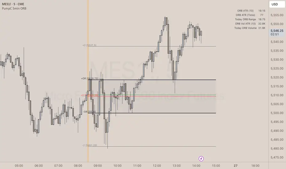
PumpC Opening Range Breakout (ORB) 5min Range📄 PumpC ORB 5-Minute Opening Range Breakout Indicator
✨ Overview
The PumpC ORB 5-Minute Opening Range Breakout indicator captures early session price action by tracking the high, low, and open of a defined 5-minute window at market open (customized for Futures or Stocks).
It plots breakout levels, extension targets, average range calculations, volume tracking, and provides visual and table-based data summaries.
This indicator is designed for traders seeking a complete, clean visualization of Opening Range Breakouts (ORB) with flexible customization.
⚙️ Main Features
Opening Range Box (ORB Box) Draws a box around the high and low of the first 5-minute session (8:30–8:35 ET for Futures, 9:30–9:35 ET for Stocks). Box extends from the session open to the session close (4:00 PM ET). Option to enable/disable historical boxes. Box color and opacity are customizable. Core ORB Levels Open Level: Plots the open price of the 5-minute ORB window. ORB Levels: Plots breakout levels at multiples: +0.5x the range +1.5x the range (customizable factor) Each level has independent color settings and visibility toggles. Option to show or hide historic extension levels. Table Display Compact table in the top-right corner showing: ORB ATR (average range) ORB ATR in ticks Today's ORB range ORB Volume ATR (average volume during ORB) Today's ORB Volume Volume is formatted automatically into "K" (thousands) or "M" (millions) for readability. Background Highlights After the ORB window closes: Blue highlight if today's ORB range is greater than the 10-day ATR average. Orange highlight if today's ORB range is smaller than the 10-day ATR average. Helps quickly assess relative strength or weakness compared to historical behavior. Alerts Breakout Confirmations: Fires when price closes above ORB High or below ORB Low. Fallout Traps: Alerts when price wick crosses ORB High/Low but closes back inside the range. Alerts use clean titles and simple messages for easy identification.
🔧 Inputs and Customization
Mode Toggle: Choose between Futures (8:30 ET open) or Stocks (9:30 ET open). Show/Hide Labels: Control label visibility for ORB and extension levels. Line Width Control: Customize thickness for ORB lines and extension levels. ORB Level Level Visibility: Independently enable or disable each extension line. Table Appearance: Customize table background color, font color, and padding. ORB Box Settings: Customize box color and control whether historical boxes are drawn.
📚 How to Use
Select Mode: Choose Futures or Stocks depending on your instrument. Observe the Opening Range: Focus on the ORB High and ORB Low during the first 5 minutes after the open. Monitor Breakouts: Breakout alerts will fire when price closes outside the ORB range, signaling potential continuation. Watch for Fallout Traps: Fallout alerts signal when price briefly wicks above/below but closes back inside the ORB range. Use Table Metrics: Instantly compare today's ORB range and volume versus historical averages to assess session strength or weakness.
🛡️ Notes
Best used on the 1-minute or 5-minute chart for intraday trading. Ensure your TradingView chart time zone is set to New York for correct functioning. Alerts must be manually configured after adding the indicator to your chart.
CyberCandle SwiftEdgeCyberCandle SwiftEdge
Overview
CyberCandle SwiftEdge is a cutting-edge, AI-inspired trading indicator designed for traders seeking precision and clarity in trend-following and swing trading. Powered by SwiftEdge, it combines Heikin Ashi candles, a gradient-colored Exponential Moving Average (EMA), and a Relative Strength Index (RSI) to deliver clear buy and sell signals. Featuring glowing visuals, dynamic signal icons, and a customizable RSI dashboard in the top-right corner, this script offers a futuristic interface for identifying high-probability trade setups on various timeframes (e.g., 1H, 4H).
What It Does
CyberCandle SwiftEdge integrates three powerful components to generate actionable trading signals:
Heikin Ashi Candles: Smooths price action to highlight trends, reducing market noise and making reversals easier to spot.
Gradient EMA: A 100-period EMA with dynamic color transitions (blue/cyan for uptrends, red/pink for downtrends) to confirm market direction.
RSI Dashboard: A neon-lit display showing RSI levels, indicating overbought (>70), oversold (<30), or neutral (30-70) conditions.
Buy and sell signals are marked with prominent, glowing icons (triangles and arrows) based on trend direction, momentum, and specific Heikin Ashi patterns. The script’s customizable parameters allow traders to tailor the strategy to their preferences, balancing signal frequency and precision.
How It Works
The strategy leverages the synergy of Heikin Ashi, EMA, and RSI to filter trades and highlight opportunities:
Trend Direction: The price must be above the EMA for buy signals (bullish trend) or below for sell signals (bearish trend). The EMA’s gradient color shifts based on its slope, visually reinforcing trend strength.
Momentum Confirmation: RSI must exceed a user-defined threshold (default: 50) for buy signals or fall below it for sell signals, ensuring momentum supports the trade.
Candle Patterns: Buy signals require a green Heikin Ashi candle (close > open), with the two prior candles having minimal upper wicks (≤5% of candle body) and being red (indicating a retracement). Sell signals require a red candle, minimal lower wicks, and two prior green candles.
RSI Dashboard: Positioned in the top-right corner, it features a glowing circle (red for overbought, green for oversold, blue for neutral), the current RSI value, and a status indicator (triangle for extremes, square for neutral). This provides instant momentum insights without cluttering the chart.
By combining Heikin Ashi’s trend clarity, EMA’s directional filter, and RSI’s momentum validation, CyberCandle SwiftEdge minimizes false signals and highlights trades with strong potential. Its vibrant, AI-like visuals make it easy to interpret at a glance.
How to Use It
Add to Chart: In TradingView, search for "CyberCandle SwiftEdge" and add it to your chart. Set the chart to Heikin Ashi candles for optimal compatibility.
Interpret Signals:
Buy Signal: Large green triangles and arrows appear below candles when the price is above the EMA, RSI is above the buy threshold (default: 50), and conditions for a bullish retracement are met. Consider entering a long position with a 1:2 risk/reward ratio.
Sell Signal: Large red triangles and arrows appear above candles when the price is below the EMA, RSI is below the sell threshold (default: 50), and conditions for a bearish retracement are met. Consider entering a short position.
RSI Dashboard: Monitor the top-right dashboard. A red circle (RSI > 70) suggests caution for buys, a green circle (RSI < 30) indicates potential buying opportunities, and a blue circle (RSI 30-70) signals neutrality.
Customize Parameters: Open the indicator’s settings to adjust:
EMA Length (default: 100): Increase (e.g., 200) for longer-term trends or decrease (e.g., 50) for shorter-term sensitivity.
RSI Length (default: 14): Adjust for more (e.g., 7) or less (e.g., 21) responsive momentum signals.
RSI Buy/Sell Thresholds (default: 50): Set higher (e.g., 55) for buys or lower (e.g., 45) for sells to require stronger momentum.
Wick Tolerance (default: 0.05): Increase (e.g., 0.1) to allow larger wicks, generating more signals, or decrease (e.g., 0.02) for stricter conditions.
Require Retracement (default: true): Disable to remove the two-candle retracement requirement, increasing signal frequency.
Trading: Use signals in conjunction with the RSI dashboard and market context. For example, avoid buy signals if the RSI dashboard is red (overbought). Always apply proper risk management, such as setting stop-losses based on recent lows/highs.
What Makes It Original
CyberCandle SwiftEdge stands out due to its futuristic, AI-inspired visual design and user-friendly customization:
Neon Aesthetics: Glowing Heikin Ashi candles, gradient EMA, and dynamic signal icons (triangles and arrows) with RSI-driven transparency create a high-tech, immersive experience.
RSI Dashboard: A compact, top-right display with a neon circle, RSI value, and adaptive status indicator (triangle/square) provides instant momentum insights without cluttering the chart.
Customizability: Users can fine-tune EMA length, RSI parameters, wick tolerance, and retracement requirements via TradingView’s settings, balancing signal frequency and precision.
Integrated Approach: The synergy of Heikin Ashi’s trend clarity, EMA’s directional strength, and RSI’s momentum validation offers a cohesive strategy that reduces false signals.
Why This Combination?
The script combines Heikin Ashi, EMA, and RSI for a complementary effect:
Heikin Ashi smooths price fluctuations, making it ideal for identifying sustained trends and retracements, which are critical for the strategy’s signal logic.
EMA provides a reliable trend filter, ensuring signals align with the broader market direction. Its gradient color enhances visual trend recognition.
RSI adds momentum context, confirming that signals occur during favorable conditions (e.g., RSI > 50 for buys). The dashboard makes RSI intuitive, even for non-technical users.
Together, these components create a balanced system that captures trend reversals after retracements, validated by momentum, with a visually engaging interface that simplifies decision-making.
Tips
Best used on volatile assets (e.g., BTC/USD, EUR/USD) and higher timeframes (1H, 4H) for clearer trends.
Experiment with parameters in the settings to match your trading style (e.g., increase wick tolerance for more signals).
Combine with other analysis (e.g., support/resistance) for higher-confidence trades.
Note
This indicator is for informational purposes and does not guarantee profits. Always backtest and use proper risk management before trading.
ScalpSwing Pro SetupScript Overview
This script is a multi-tool setup designed for both scalping (1m–5m) and swing trading (1H–4H–Daily). It combines the power of trend-following , momentum , and mean-reversion tools:
What’s Included in the Script
1. EMA Indicators (20, 50, 200)
- EMA 20 (blue) : Short-term trend
- EMA 50 (orange) : Medium-term trend
- EMA 200 (red) : Long-term trend
- Use:
- EMA 20 crossing above 50 → bullish trend
- EMA 20 crossing below 50 → bearish trend
- Price above 200 EMA = uptrend bias
2. VWAP (Volume Weighted Average Price)
- Shows the average price weighted by volume
- Best used in intraday (1m to 15m timeframes)
- Use:
- Price bouncing from VWAP = reversion trade
- Price far from VWAP = likely pullback incoming
3. RSI (14) + Key Levels
- Shows momentum and overbought/oversold zones
- Levels:
- 70 = Overbought (potential sell)
- 30 = Oversold (potential buy)
- 50 = Trend confirmation
- Use:
- RSI 30–50 in uptrend = dip buying zone
- RSI 70–50 in downtrend = pullback selling zone
4. MACD Crossovers
- Standard MACD with histogram & cross alerts
- Shows trend momentum shifts
- Green triangle = Bullish MACD crossover
- Red triangle = Bearish MACD crossover
- Use:
- Confirm swing trades with MACD crossover
- Combine with RSI divergence
5. Buy & Sell Signal Logic
BUY SIGNAL triggers when:
- EMA 20 crosses above EMA 50
- RSI is between 50 and 70 (momentum bullish, not overbought)
SELL SIGNAL triggers when:
- EMA 20 crosses below EMA 50
- RSI is between 30 and 50 (bearish momentum, not oversold)
These signals appear as:
- BUY : Green label below the candle
- SELL : Red label above the candle
How to Trade with It
For Scalping (1m–5m) :
- Focus on EMA crosses near VWAP
- Confirm with RSI between 50–70 (buy) or 50–30 (sell)
- Use MACD triangle as added confluence
For Swing (1H–4H–Daily) :
- Look for EMA 20–50 cross + price above EMA 200
- Confirm trend with MACD and RSI
- Trade breakout or pullback depending on structure
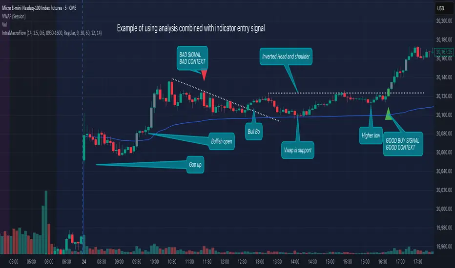
Intraday Macro & Flow Indicator# IntraMacroFlow Indicator
## Introduction
IntraMacroFlow is a volume and delta-based indicator that identifies significant price movements within trading sessions. It generates signals when volume spikes coincide with quality price movement, filtered by RSI to avoid overbought/oversold conditions.
> **Note:** This indicator provides multiple signals and should be combined with additional analysis methods such as support/resistance, trend direction, and price action patterns.
## Inputs
### Volume Settings
* **Volume Lookback Period** (14) - Number of bars for volume moving average calculation
* **Volume Threshold Multiplier** (1.5) - Required volume increase over average to generate signals
* **Delta Threshold** (0.3) - Required close-to-open movement relative to bar range (higher = stronger movement)
### Session Configuration
* **Use Dynamic Session Detection** (true) - Automatically determine session times
* **Highlight Market Open Period** (true) - Highlight first third of trading session
* **Highlight Mid-Session Period** (true) - Highlight middle portion of trading session
* **Detect Signals Throughout Whole Session** (true) - Find signals in entire session
* **Session Time** ("0930-1600") - Trading hours in HHMM-HHMM format
* **Session Type** ("Regular") - Select Regular, Extended, or Custom session
### Manual Session Settings
Used when dynamic detection is disabled:
* **Manual Session Open Hour** (9)
* **Manual Session Open Minute** (30)
* **Manual Session Open Duration** (60)
* **Manual Mid-Session Start Hour** (12)
* **Manual Mid-Session End Hour** (14)
## How It Works
The indicator analyzes each bar using three primary conditions:
1. **Volume Condition**: Current volume > Average volume × Threshold
2. **Delta Condition**: |Close-Open|/Range > Delta threshold
3. **Time Condition**: Bar falls within configured session times
When all conditions are met:
* Bullish signals appear when close > open and RSI < 70
* Bearish signals appear when close < open and RSI > 30
## Display Elements
### Shapes and Colors
* Green triangles below bars - Bullish signals
* Red triangles above bars - Bearish signals
* Blue background - Market open period
* Purple background - Mid-session period
* Bar coloring - Green (bullish), Red (bearish), or unchanged
### Information Panel
A dynamic label shows:
* Current volume relative to average (Vol)
* Delta value for current bar (Delta)
* RSI value (RSI)
* Session status (Active/Closed)
## Calculation Method
```
// Volume Condition
volumeMA = ta.sma(volume, lookbackPeriod)
volumeCondition = volume > volumeMA * volumeThreshold
// Delta Calculation (price movement quality)
priceRange = high - low
delta = math.abs(close - open) / priceRange
deltaCondition = delta > deltaThreshold
// Direction and RSI Filter
bullishBias = close > open and entrySignal and not (rsi > 70)
bearishBias = close < open and entrySignal and not (rsi < 30)
```
## Usage Recommendations
### Suitable Markets
* Equities during regular trading hours
* Futures markets
* Forex during active sessions
* Cryptocurrencies with defined volume patterns
### Recommended Timeframes
* 1-minute to 1-hour (optimal: 5 or 15-minute)
### Parameter Adjustments
* For fewer but stronger signals: increase Volume Threshold (2.0+) and Delta Threshold (0.4-0.6)
* For more signals: decrease Volume Threshold (1.2-1.5) and Delta Threshold (0.2-0.3)
### Usage Tips
* Combine with trend analysis for higher-probability entries
* Focus on signals occurring at session boundaries and mid-session
* Use opposite signals as potential exit points
* Configure alerts to receive notifications when signals occur
## Additional Notes
* RSI parameters are fixed at 14 periods with 70/30 thresholds
* The indicator handles overnight sessions correctly
* Fully compatible with TradingView alerts
* Customizable visual elements
## Release Notes
Initial release: This is a template indicator that should be customized to suit your specific trading strategies and preferences.
Session Color Blocks🧠 Purpose:
To visually highlight different market sessions — Asia, London, Premarket (US), and New York — using colored background blocks on the chart for better timing, context, and trade planning.
🕓 Session Times Used (Eastern Time / New York Time):
Session Time (ET) Color
Asia 8:00 PM – 3:00 AM 🟨 Yellow
London 3:00 AM – 8:30 AM 🟥 Red
Premarket 8:30 AM – 9:30 AM 🟦 Blue
New York 9:30 AM – 4:00 PM 🟩 Green
(DST is automatically handled via "America/New_York" timezone)
✅ Features:
Session colors appear only when that session is active.
Sessions are mutually exclusive, so no overlapping blocks.
Works on any symbol, especially useful for US stock/futures traders.
Auto-adjusts for daylight savings (using TradingView's IANA timezones).
🔧 Future Enhancements (Optional):
Toggle each session on/off
Add vertical lines or labels for session opens
Extend to weekends or custom sessions

Strategy Stats [presentTrading]Hello! it's another weekend. This tool is a strategy performance analysis tool. Looking at the TradingView community, it seems few creators focus on this aspect. I've intentionally created a shared version. Welcome to share your idea or question on this.
█ Introduction and How it is Different
Strategy Stats is a comprehensive performance analytics framework designed specifically for trading strategies. Unlike standard strategy backtesting tools that simply show cumulative profits, this analytics suite provides real-time, multi-timeframe statistical analysis of your trading performance.
Multi-timeframe analysis: Automatically tracks performance metrics across the most recent time periods (last 7 days, 30 days, 90 days, 1 year, and 4 years)
Advanced statistical measures: Goes beyond basic metrics to include Information Coefficient (IC) and Sortino Ratio
Real-time feedback: Updates performance statistics with each new trade
Visual analytics: Color-coded performance table provides instant visual feedback on strategy health
Integrated risk management: Implements sophisticated take profit mechanisms with 3-step ATR and percentage-based exits
BTCUSD Performance
The table in the upper right corner is a comprehensive performance dashboard showing trading strategy statistics.
Note: While this presentation uses Vegas SuperTrend as the underlying strategy, this is merely an example. The Stats framework can be applied to any trading strategy. The Vegas SuperTrend implementation is included solely to demonstrate how the analytics module integrates with a trading strategy.
⚠️ Timeframe Limitations
Important: TradingView's backtesting engine has a maximum storage limit of 10,000 bars. When using this strategy stats framework on smaller timeframes such as 1-hour or 2-hour charts, you may encounter errors if your backtesting period is too long.
Recommended Timeframe Usage:
Ideal for: 4H, 6H, 8H, Daily charts and above
May cause errors on: 1H, 2H charts spanning multiple years
Not recommended for: Timeframes below 1H with long history
█ Strategy, How it Works: Detailed Explanation
The Strategy Stats framework consists of three primary components: statistical data collection, performance analysis, and visualization.
🔶 Statistical Data Collection
The system maintains several critical data arrays:
equityHistory: Tracks equity curve over time
tradeHistory: Records profit/loss of each trade
predictionSignals: Stores trade direction signals (1 for long, -1 for short)
actualReturns: Records corresponding actual returns from each trade
For each closed trade, the system captures:
float tradePnL = strategy.closedtrades.profit(tradeIndex)
float tradeReturn = strategy.closedtrades.profit_percent(tradeIndex)
int tradeType = entryPrice < exitPrice ? 1 : -1 // Direction
🔶 Performance Metrics Calculation
The framework calculates several key performance metrics:
Information Coefficient (IC):
The correlation between prediction signals and actual returns, measuring forecast skill.
IC = Correlation(predictionSignals, actualReturns)
Where Correlation is the Pearson correlation coefficient:
Correlation(X,Y) = (nΣXY - ΣXY) / √
Sortino Ratio:
Measures risk-adjusted return focusing only on downside risk:
Sortino = (Avg_Return - Risk_Free_Rate) / Downside_Deviation
Where Downside Deviation is:
Downside_Deviation = √
R_i represents individual returns, T is the target return (typically the risk-free rate), and n is the number of observations.
Maximum Drawdown:
Tracks the largest percentage drop from peak to trough:
DD = (Peak_Equity - Trough_Equity) / Peak_Equity * 100
🔶 Time Period Calculation
The system automatically determines the appropriate number of bars to analyze for each timeframe based on the current chart timeframe:
bars_7d = math.max(1, math.round(7 * barsPerDay))
bars_30d = math.max(1, math.round(30 * barsPerDay))
bars_90d = math.max(1, math.round(90 * barsPerDay))
bars_365d = math.max(1, math.round(365 * barsPerDay))
bars_4y = math.max(1, math.round(365 * 4 * barsPerDay))
Where barsPerDay is calculated based on the chart timeframe:
barsPerDay = timeframe.isintraday ?
24 * 60 / math.max(1, (timeframe.in_seconds() / 60)) :
timeframe.isdaily ? 1 :
timeframe.isweekly ? 1/7 :
timeframe.ismonthly ? 1/30 : 0.01
🔶 Visual Representation
The system presents performance data in a color-coded table with intuitive visual indicators:
Green: Excellent performance
Lime: Good performance
Gray: Neutral performance
Orange: Mediocre performance
Red: Poor performance
█ Trade Direction
The Strategy Stats framework supports three trading directions:
Long Only: Only takes long positions when entry conditions are met
Short Only: Only takes short positions when entry conditions are met
Both: Takes both long and short positions depending on market conditions
█ Usage
To effectively use the Strategy Stats framework:
Apply to existing strategies: Add the performance tracking code to any strategy to gain advanced analytics
Monitor multiple timeframes: Use the multi-timeframe analysis to identify performance trends
Evaluate strategy health: Review IC and Sortino ratios to assess predictive power and risk-adjusted returns
Optimize parameters: Use performance data to refine strategy parameters
Compare strategies: Apply the framework to multiple strategies to identify the most effective approach
For best results, allow the strategy to generate sufficient trade history for meaningful statistical analysis (at least 20-30 trades).
█ Default Settings
The default settings have been carefully calibrated for cryptocurrency markets:
Performance Tracking:
Time periods: 7D, 30D, 90D, 1Y, 4Y
Statistical measures: Return, Win%, MaxDD, IC, Sortino Ratio
IC color thresholds: >0.3 (green), >0.1 (lime), <-0.1 (orange), <-0.3 (red)
Sortino color thresholds: >1.0 (green), >0.5 (lime), <0 (red)
Multi-Step Take Profit:
ATR multipliers: 2.618, 5.0, 10.0
Percentage levels: 3%, 8%, 17%
Short multiplier: 1.5x (makes short take profits more aggressive)
Stop loss: 20%

New York Open LinesThis indicator marks key New York trading session opens on the chart. It draws horizontal lines at the New York Midnight Open (00:00 NY time) and the New York Economic Open (08:30 NY time) prices.
Key Features:
1) Customizable Line Styles & Colors:
* Users can choose between solid, dotted, or dashed lines.
* Colors are customizable for each open level.
2) Timeframe-Based Logic:
* For timeframes above 30 minutes:
- It retrieves the midnight (NYMO) and 8:30 AM (ETO) open prices using request.security_lower_tf().
- The script ensures the price is stored only once per day.
* For 30-minute timeframes and below:
- The script draws lines at the exact open prices as bars appear.
3) Line Management:
* The lines extend for 24 hours from the open.
* The previous day's lines are removed to keep the chart clean.
4) Session Reset:
* At the start of a new trading day, the stored NYMO and ETO prices reset to na to prepare for the next session.
This helps traders quickly identify key New York session levels, often used for support, resistance, and breakout trading strategies.
MTF Moving Averages (only EMA)MTF Moving Averages (only EMA)
This script provides a Multi-Timeframe (MTF) Exponential Moving Average (EMA) indicator for traders to visualize multiple EMAs across different timeframes directly on a single chart.
The indicator dynamically calculates and plots up to four EMAs per timeframe (15-minute, 30-minute, 1-hour, and Daily) with user-defined lengths, offering valuable insight into price trends and potential entry or exit points.
Key Features:
Multiple Timeframe Support: The script allows you to view EMAs from different timeframes simultaneously. This is especially useful for traders who follow trends across different timeframes to make more informed decisions.
Customizable Lengths: For each timeframe, the lengths of the EMAs are fully customizable. You can adjust the length of up to four EMAs per timeframe to suit your strategy.
EMA Calculation: The Exponential Moving Average (EMA) is used, which gives more weight to recent prices and reacts faster to price changes compared to the simple moving average (SMA).
Timeframe Flexibility: The indicator supports the following timeframes:
15-minute: Ideal for short-term traders and scalpers.
30-minute: For intraday trading with a slightly longer perspective.
1-hour: Suitable for swing traders and those who prefer a more medium-term view.
Daily: Great for longer-term trend-following strategies.
Interactive and User-Friendly: You can toggle the visibility of each EMA on each timeframe, allowing you to choose exactly which EMAs you wish to display, depending on your trading strategy.
Color-Coded for Clarity: The script uses distinct colors for each EMA on the chart:
Blue: EMA1
Green: EMA2
Red: EMA3
Purple: EMA4
Line Width Customization: Each plotted EMA line has a customizable width for better visual clarity.
Use Case:
Traders who use multiple timeframes for analysis (e.g., those using the "multi-timeframe analysis" technique) will find this script particularly useful. For example, a trader may look at the 15-minute chart to catch short-term movements, the 30-minute chart for intraday trends, the 1-hour chart for swing positions, and the Daily chart for identifying the overarching market trend. The script enables them to view the EMAs for all these timeframes in one glance without having to manually switch between them.
By observing the relationships between EMAs across multiple timeframes, traders can gain valuable insights into market conditions such as:
Crossovers: When a shorter-term EMA crosses above or below a longer-term EMA, it can signal a potential trend reversal or continuation.
Trend Strength: Multiple EMAs in alignment across different timeframes can indicate strong trend strength.
Support and Resistance: EMAs can act as dynamic support and resistance levels, guiding traders on price action levels to watch for potential price reversals.
Instructions:
Enable/Disable EMAs: Toggle on or off the EMAs for each timeframe (15-min, 30-min, 1-hour, Daily) using the script’s settings.
Adjust EMA Lengths: Change the default lengths for each EMA to match your preferred settings for different timeframes.
Monitor Key Levels: Watch how price interacts with the plotted EMAs to spot potential trading signals based on your strategy.
This indicator is designed to enhance your multi-timeframe analysis and help make more informed, data-driven trading decisions.
Midnight Opening Ranges[TDL]Midnight Opening Range Indicator for TradingView
Description:
The Midnight Opening Range Indicator as taught by Micheal J. Huddleston is a powerful tool designed for traders who want to analyze price action during the critical midnight to 00:30 timeframe. This indicator highlights the opening range for both the current day and previous days, providing valuable insights into market behavior during this specific period. It also calculates and displays deviations from the opening range, as well as allows for custom opening prices to be set, making it highly adaptable to your trading strategy.
Key Features:
Today's Opening Range (00:00 - 00:30):
The indicator plots the high and low of the price range between 00:00 and 00:30 for the current day.
This range is highlighted on the chart, making it easy to identify the initial market movement and potential support/resistance levels.
Previous Days' Opening Ranges:
The indicator also displays the opening ranges for previous days, allowing you to how price reacts off of previous days ranges not just todays.
This feature helps in identifying patterns or recurring behaviors in the market in which price uses this range and previous days ranges throughout the trading day.
Deviations from the Opening Range:
The indicator calculates and plots deviations from the opening range, both above and below the high and low of the range.
These deviations can be used to identify potential breakout or reversal points, giving you an edge in anticipating market moves.
Custom Opening Prices:
The indicator allows you to set custom opening prices, which can be useful if you want to analyze the market based on a specific reference point rather than the default midnight opening.
This feature is particularly useful for traders who follow alternative trading sessions or have specific entry criteria.
Customizable Visuals:
The indicator offers customizable colors and styles for the opening range, deviations, and custom opening prices, allowing you to tailor the visual representation to your preferences.
How to Use:
Identify Key Levels: Use the highlighted opening range to identify key support and resistance levels for the day.
Monitor Deviations: Watch for price movements beyond the opening range deviations to spot potential breakouts or reversals.
Previous Range Data: Use previous days to identify areas of potential AMD.
Set Custom Prices: Adjust the custom opening price to align with your trading strategy or session preferences.
Ideal For:
Day Traders: Perfect for traders who focus on the early hours of the market to capture initial momentum.
Swing Traders: Useful for identifying key levels that could influence price action over several days.
Algorithmic Traders: Can be integrated into automated trading systems to trigger trades based on the opening range and deviations.
Conclusion:
The Midnight Opening Range Indicator is an essential tool for any trader looking to gain an edge in the market by focusing on the critical midnight to 00:30 timeframe. With its ability to highlight opening ranges, calculate deviations, and accommodate custom opening prices, this indicator provides a comprehensive view of market behavior during this pivotal period. Whether you're a day trader, swing trader, or algorithmic trader, this indicator will help you make more informed trading decisions.

ORB with 100 EMAORB Trading Strategy for FX Pairs on the 30-Minute Time Frame
Overview
This Opening Range Breakout (ORB) strategy is designed for trading FX pairs on the 30-minute time frame. The strategy is structured to take advantage of price momentum while aligning trades with the overall trend using the 100-period Exponential Moving Average (100EMA). The primary objective is to enter trades when price breaks and closes above or below the Opening Range (OR), with additional confirmation from a retest of the OR level if the initial entry is missed.
Strategy Rules
1. Defining the Opening Range (OR)
- The OR is determined by the high and low of the first 30-minute candle after market open.
- This range acts as the key level for breakout trading.
2. Trend Confirmation Using the 100EMA
- The 100EMA serves as a filter to determine trade direction:
- Buy Setup: Only take buy trades when the OR is above the 100EMA.
- Sell Setup: Only take sell trades when the OR is below the 100EMA.
3. Entry Criteria
- Buy Trade: Enter a long position when a candle breaks and closes above the OR high, confirming the breakout.
- Sell Trade: Enter a short position when a candle breaks and closes below the OR low, confirming the breakout.
- Retest Entry: If the initial entry is missed, wait for a price retest of the OR level for a secondary entry opportunity.
4. Risk-to-Reward Ratio (R2R)
- The goal is to target a 1:1 Risk-to-Reward (R2R) ratio.
- Stop-loss placement:
- Buy Trade: Place stop-loss just below the OR low.
- Sell Trade: Place stop-loss just above the OR high.
- Take profit at a distance equal to the stop-loss for a 1:1 R2R.
5. Risk Management
- Risk per trade should be based on personal risk tolerance.
- Adjust lot sizes accordingly to maintain a controlled risk percentage of account balance.
- Avoid over-leveraging, and consider moving stop-loss to breakeven if the price moves favourably.
Additional Considerations
- Avoid trading during major news events that may cause high volatility and unpredictable price movements.
- Monitor market conditions to ensure breakout confirmation with strong momentum rather than false breakouts.
- Use additional confluences such as candlestick patterns, support/resistance zones, or volume analysis for stronger trade validation.
This ORB strategy is designed to provide structured trade opportunities by combining breakout momentum with trend confirmation via the 100EMA. The strategy is straightforward, allowing traders to capitalise on clear breakout movements while implementing effective risk management practices. While the 1:1 R2R target provides a balanced approach, traders should always adapt their risk tolerance and market conditions to optimise trade performance.
By following these rules and maintaining discipline, traders can use this strategy effectively across various FX pairs on the 30-minute time frame.
Average Price in Time PeriodsThis Pine Script calculates and displays average prices for two specific time ranges during a trading day: from 09:00 to 22:30 and from 22:30 to 09:00. It updates the average prices by summing the closing prices in each time frame and then plots them as green and red lines, respectively. The script also displays black lines outside these specific time ranges to prevent "gaps" in the chart during off-peak hours. The displayed lines are dynamically adjusted based on the current time, with the green line for 09:00-22:30 and the red line for 22:30-09:00.

SV Volatility Indicator BasicThe SV Volatility Indicator Basic in TradingView calculates and visualizes daily and average volatility over specified periods using three lines. Here’s what it does:
1. Daily Volatility Calculation. The indicator computes daily volatility as the percentage difference between the high and low prices relative to the closing price:
2. 30-day Moving Average of Volatility. A simple moving average (SMA) is applied to the daily volatility values over the last 30 days to smooth short-term fluctuations.
3. 90-day Moving Average of Volatility. Similarly, an SMA is calculated over the last 90 days to provide a longer-term view of volatility trends.
4. Visualization:
Three lines are plotted:
Red line: Represents the daily volatility in percentage terms.
Blue line: Displays the 30-day moving average of volatility.
Green line: Shows the 90-day moving average of volatility.
This indicator helps traders analyze market volatility by providing both immediate (daily) and smoothed (30-day and 90-day) measures, aiding in trend identification and risk assessment.

NVOL Normalized Volume & VolatilityOVERVIEW
Plots a normalized volume (or volatility) relative to a given bar's typical value across all charted sessions. The concept is similar to Relative Volume (RVOL) and Average True Range (ATR), but rather than using a moving average, this script uses bar data from previous sessions to more accurately separate what's normal from what's anomalous. Compatible on all timeframes and symbols.
Having volume and volatility processed within a single indicator not only allows you to toggle between the two for a consistent data display, it also allows you to measure how correlated they are. These measurements are available in the data table.
DATA & MATH
The core formula used to normalize each bar is:
( Value / Basis ) × Scale
Value
The current bar's volume or volatility (see INPUTS section). When set to volume, it's exactly what you would expect (the volume of the bar). When set to volatility, it's the bar's range (high - low).
Basis
A statistical threshold (Mean, Median, or Q3) plus a Sigma multiple (standard deviations). The default is set to the Mean + Sigma × 3 , which represents 99.7% of data in a normal distribution. The values are derived from the current bar's equivalent in other sessions. For example, if the current bar time is 9:30 AM, all previous 9:30 AM bars would be used to get the Mean and Sigma. Thus Mean + Sigma × 3 would represent the Normal Bar Vol at 9:30 AM.
Scale
Depends on the Normalize setting, where it is 1 when set to Ratio, and 100 when set to Percent. This simply determines the plot's scale (ie. 0 to 1 vs. 0 to 100).
INPUTS
While the default configuration is recommended for a majority of use cases (see BEST PRACTICES), settings should be adjusted so most of the Normalized Plot and Linear Regression are below the Signal Zone. Only the most extreme values should exceed this area.
Normalize
Allows you to specify what should be normalized (Volume or Volatility) and how it should be measured (as a Ratio or Percentage). This sets the value and scale in the core formula.
Basis
Specifies the statistical threshold (Mean, Median, or Q3) and how many standard deviations should be added to it (Sigma). This is the basis in the core formula.
Mean is the sum of values divided by the quantity of values. It's what most people think of when they say "average."
Median is the middle value, where 50% of the data will be lower and 50% will be higher.
Q3 is short for Third Quartile, where 75% of the data will be lower and 25% will be higher (think three quarters).
Sample
Determines the maximum sample size.
All Charted Bars is the default and recommended option, and ignores the adjacent lookback number.
Lookback is not recommended, but it is available for comparisons. It uses the adjacent lookback number and is likely to produce unreliable results outside a very specific context that is not suitable for most traders. Normalization is not a moving average. Unless you have a good reason to limit the sample size, do not use this option and instead use All Charted Bars .
Show Vol. name on plot
Overlays "VOLUME" or "VOLATILITY" on the plot (whichever you've selected).
Lin. Reg.
Polynomial regressions are great for capturing non-linear patterns in data. TradingView offers a "linear regression curve", which this script uses as a substitute. If you're unfamiliar with either term, think of this like a better moving average.
You're able to specify the color, length, and multiple (how much to amplify the value). The linear regression derives its value from the normalized values.
Norm. Val.
This is the color of the normalized value of the current bar (see DATA & MATH section). You're able to specify the default, within signal, and beyond signal colors. As well as the plot style.
Fade in colors between zero and the signal
Programmatically adjust the opacity of the primary plot color based on it's normalized value. When enabled, values equal to 0 will be fully transparent, become more opaque as they move away from 0, and be fully opaque at the signal. Adjusting opacity in this way helps make difference more obvious.
Plot relative to bar direction
If enabled, the normalized value will be multiplied by -1 when a bar's open is greater than the bar's close, mirroring price direction.
Technically volume and volatility are directionless. Meaning there's really no such thing as buy volume, sell volume, positive volatility, or negative volatility. There is just volume (1 buy = 1 sell = 1 volume) and volatility (high - low). Even so, visually reflecting the net effect of pricing pressure can still be useful. That's all this setting does.
Sig. Zone
Signal zones make identifying extremes easier. They do not signal if you should buy or sell, only that the current measurement is beyond what's normal. You are able to adjust the color and bounds of the zone.
Int. Levels
Interim levels can be useful when you want to visually bracket values into high / medium / low. These levels can have a value anywhere between 0 and 1. They will automatically be multiplied by 100 when the scale is set to Percent.
Zero Line
This setting allows you to specify the visibility of the zero line to best suit your trading style.
Volume & Volatility Stats
Displays a table of core values for both volume and volatility. Specifically the actual value, threshold (mean, median, or Q3), sigma (standard deviation), basis, normalized value, and linear regression.
Correlation Stats
Displays a table of correlation statistics for the current bar, as well as the data set average. Specifically the coefficient, R2, and P-Value.
Indices & Sample Size
Displays a table of mixed data. Specifically the current bar's index within the session, the current bar's index within the sample, and the sample size used to normalize the current bar's value.
BEST PRACTICES
NVOL can tell you what's normal for 9:30 AM. RVOL and ATR can only tell you if the current value is higher or lower than a moving average.
In a normal distribution (bell curve) 99.7% of data occurs within 3 standard deviations of the mean. This is why the default basis is set to "Mean, 3"; it includes the typical day-to-day fluctuations, better contextualizing what's actually normal, minimizing false positives.
This means a ratio value greater than 1 only occurs 0.3% of the time. A series of these values warrants your attention. Which is why the default signal zone is between 1 and 2. Ratios beyond 2 would be considered extreme with the default settings.
Inversely, ratio values less than 1 (the normal daily fluctuations) also tell a story. We should expect most values to occur around the middle 3rd, which is why interim levels default to 0.33 and 0.66, visually simplifying a given move's participation. These can be set to whatever you like and only serve as visual aids for your specific trading style.
It's worth noting that the linear regression oscillates when plotted directionally, which can help clarify short term move exhaustion and continuation. Akin to a relative strength index (RSI), it may be used to inform a trading decision, but it should not be the only factor.
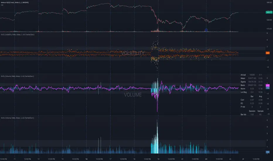
AI indicatorThis script is a trading indicator designed for future trading signals on the TradingView platform. It uses a combination of the Relative Strength Index (RSI) and a Simple Moving Average (SMA) to generate buy and sell signals. Here's a breakdown of its components and logic:
1. Inputs
The script includes configurable inputs to make it adaptable for different market conditions:
RSI Length: Determines the number of periods for calculating RSI. Default is 14.
RSI Overbought Level: Signals when RSI is above this level (default 70), indicating potential overbought conditions.
RSI Oversold Level: Signals when RSI is below this level (default 30), indicating potential oversold conditions.
Moving Average Length: Defines the SMA length used to confirm price trends (default 50).
2. Indicators Used
RSI (Relative Strength Index):
Measures the speed and change of price movements.
A value above 70 typically indicates overbought conditions.
A value below 30 typically indicates oversold conditions.
SMA (Simple Moving Average):
Used to smooth price data and identify trends.
Price above the SMA suggests an uptrend, while price below suggests a downtrend.
3. Buy and Sell Signal Logic
Buy Condition:
The RSI value is below the oversold level (e.g., 30), indicating the market might be undervalued.
The current price is above the SMA, confirming an uptrend.
Sell Condition:
The RSI value is above the overbought level (e.g., 70), indicating the market might be overvalued.
The current price is below the SMA, confirming a downtrend.
These conditions ensure that trades align with market trends, reducing false signals.
4. Visual Features
Buy Signals: Displayed as green labels (plotshape) below the price bars when the buy condition is met.
Sell Signals: Displayed as red labels (plotshape) above the price bars when the sell condition is met.
Moving Average Line: A blue line (plot) added to the chart to visualize the SMA trend.
5. How It Works
When the buy condition is true (RSI < 30 and price > SMA), a green label appears below the corresponding price bar.
When the sell condition is true (RSI > 70 and price < SMA), a red label appears above the corresponding price bar.
The blue SMA line helps to visualize the overall trend and acts as confirmation for signals.
6. Advantages
Combines Momentum and Trend Analysis:
RSI identifies overbought/oversold conditions.
SMA confirms whether the market is trending up or down.
Simple Yet Effective:
Reduces noise by using well-established indicators.
Easy to interpret for beginners and experienced traders alike.
Customizable:
Parameters like RSI length, oversold/overbought levels, and SMA length can be adjusted to fit different assets or timeframes.
7. Limitations
Lagging Indicator: SMA is a lagging indicator, so it may not capture rapid market reversals quickly.
Not Foolproof: No trading indicator can guarantee 100% accuracy. False signals can occur in choppy or sideways markets.
Needs Volume Confirmation: The script does not consider trading volume, which could enhance signal reliability.
8. How to Use It
Copy the script into TradingView's Pine Editor.
Save and add it to your chart.
Adjust the RSI and SMA parameters to suit your preferred asset and timeframe.
Look for buy signals (green labels) in uptrends and sell signals (red labels) in downtrends.

[blackcat] L3 Counter Peacock Spread█ OVERVIEW
The script titled " L3 Counter Peacock Spread" is an indicator designed for use in TradingView. It calculates and plots various moving averages, K lines derived from these moving averages, additional simple moving averages (SMAs), weighted moving averages (WMAs), and other technical indicators like slope calculations. The primary function of the script is to provide a comprehensive set of visual tools that traders can use to identify trends, potential support/resistance levels, and crossover signals.
█ LOGICAL FRAMEWORK
Input Parameters:
There are no explicit input parameters defined; all variables are hardcoded or calculated within the script.
Calculations:
• Moving Averages: Calculates Simple Moving Averages (SMA) using ta.sma.
• Slope Calculation: Computes the slope of a given series over a specified period using linear regression (ta.linreg).
• K Lines: Defines multiple exponentially adjusted SMAs based on a 30-period MA and a 1-period MA.
• Weighted Moving Average (WMA): Custom function to compute WMAs by iterating through price data points.
• Other Indicators: Includes Exponential Moving Average (EMA) for momentum calculation.
Plotting:
Various elements such as MAs, K lines, conditional bands, additional SMAs, and WMAs are plotted on the chart overlaying the main price action.
No loops control the behavior beyond those used in custom functions for calculating WMAs. Conditional statements determine the coloring of certain plot lines based on specific criteria.
█ CUSTOM FUNCTIONS
calculate_slope(src, length) :
• Purpose: To calculate the slope of a time-series data point over a specified number of periods.
• Functionality: Uses linear regression to find the current and previous slopes and computes their difference scaled by the timeframe multiplier.
• Parameters:
– src: Source of the input data (e.g., closing prices).
– length: Periodicity of the linreg calculation.
• Return Value: Computed slope value.
calculate_ma(source, length) :
• Purpose: To calculate the Simple Moving Average (SMA) of a given source over a specified period.
• Functionality: Utilizes TradingView’s built-in ta.sma function.
• Parameters:
– source: Input data series (e.g., closing prices).
– length: Number of bars considered for the SMA calculation.
• Return Value: Calculated SMA value.
calculate_k_lines(ma30, ma1) :
• Purpose: Generates multiple exponentially adjusted versions of a 30-period MA relative to a 1-period MA.
• Functionality: Multiplies the 30-period MA by coefficients ranging from 1.1 to 3 and subtracts multiples of the 1-period MA accordingly.
• Parameters:
– ma30: 30-period Simple Moving Average.
– ma1: 1-period Simple Moving Average.
• Return Value: Returns an array containing ten different \u2003\u2022 "K line" values.
calculate_wma(source, length) :
• Purpose: Computes the Weighted Moving Average (WMA) of a provided series over a defined period.
• Functionality: Iterates backward through the last 'n' bars, weights each bar according to its position, sums them up, and divides by the total weight.
• Parameters:
– source: Price series to average.
– length: Length of the lookback window.
• Return Value: Calculated WMA value.
█ KEY POINTS AND TECHNIQUES
• Advanced Pine Script Features: Utilization of custom functions for encapsulating complex logic, leveraging TradingView’s library functions (ta.sma, ta.linreg, ta.ema) for efficient computations.
• Optimization Techniques: Efficient computation of K lines via pre-calculated components (multiples of MA30 and MA1). Use of arrays to store intermediate results which simplifies plotting.
• Best Practices: Clear separation between calculation and visualization sections enhances readability and maintainability. Usage of color.new() allows dynamic adjustments without hardcoding colors directly into plot commands.
• Unique Approaches: Introduction of K lines provides an alternative representation of trend strength compared to traditional MAs. Implementation of conditional band coloring adds real-time context to existing visual cues.
█ EXTENDED KNOWLEDGE AND APPLICATIONS
Potential Modifications/Extensions:
• Adding more user-defined inputs for lengths of MAs, K lines, etc., would make the script more flexible.
• Incorporating alert conditions based on crossovers between key lines could enhance automated trading strategies.
Application Scenarios:
• Useful for both intraday and swing trading due to the combination of short-term and long-term MAs along with trend analysis via slopes and K lines.
• Can be integrated into larger systems combining this indicator with others like oscillators or volume-based metrics.
Related Concepts:
• Understanding how linear regression works internally aids in grasping the slope calculation.
• Familiarity with WMA versus SMA helps appreciate why different types of averaging might be necessary depending on market dynamics.
• Knowledge of candlestick patterns can complement insights gained from this indicator.