TA█ TA Library
📊 OVERVIEW
TA is a Pine Script technical analysis library. This library provides 25+ moving averages and smoothing filters , from classic SMA/EMA to Kalman Filters and adaptive algorithms, implemented based on academic research.
🎯 Core Features
Academic Based - Algorithms follow original papers and formulas
Performance Optimized - Pre-calculated constants for faster response
Unified Interface - Consistent function design
Research Based - Integrates technical analysis research
🎯 CONCEPTS
Library Design Philosophy
This technical analysis library focuses on providing:
Academic Foundation
Algorithms based on published research papers and academic standards
Implementations that follow original mathematical formulations
Clear documentation with research references
Developer Experience
Unified interface design for consistent usage patterns
Pre-calculated constants for optimal performance
Comprehensive function collection to reduce development time
Single import statement for immediate access to all functions
Each indicator encapsulated as a simple function call - one line of code simplifies complexity
Technical Excellence
25+ carefully implemented moving averages and filters
Support for advanced algorithms like Kalman Filter and MAMA/FAMA
Optimized code structure for maintainability and reliability
Regular updates incorporating latest research developments
🚀 USING THIS LIBRARY
Import Library
//@version=6
import DCAUT/TA/1 as dta
indicator("Advanced Technical Analysis", overlay=true)
Basic Usage Example
// Classic moving average combination
ema20 = ta.ema(close, 20)
kama20 = dta.kama(close, 20)
plot(ema20, "EMA20", color.red, 2)
plot(kama20, "KAMA20", color.green, 2)
Advanced Trading System
// Adaptive moving average system
kama = dta.kama(close, 20, 2, 30)
= dta.mamaFama(close, 0.5, 0.05)
// Trend confirmation and entry signals
bullTrend = kama > kama and mamaValue > famaValue
bearTrend = kama < kama and mamaValue < famaValue
longSignal = ta.crossover(close, kama) and bullTrend
shortSignal = ta.crossunder(close, kama) and bearTrend
plot(kama, "KAMA", color.blue, 3)
plot(mamaValue, "MAMA", color.orange, 2)
plot(famaValue, "FAMA", color.purple, 2)
plotshape(longSignal, "Buy", shape.triangleup, location.belowbar, color.green)
plotshape(shortSignal, "Sell", shape.triangledown, location.abovebar, color.red)
📋 FUNCTIONS REFERENCE
ewma(source, alpha)
Calculates the Exponentially Weighted Moving Average with dynamic alpha parameter.
Parameters:
source (series float) : Series of values to process.
alpha (series float) : The smoothing parameter of the filter.
Returns: (float) The exponentially weighted moving average value.
dema(source, length)
Calculates the Double Exponential Moving Average (DEMA) of a given data series.
Parameters:
source (series float) : Series of values to process.
length (simple int) : Number of bars for the moving average calculation.
Returns: (float) The calculated Double Exponential Moving Average value.
tema(source, length)
Calculates the Triple Exponential Moving Average (TEMA) of a given data series.
Parameters:
source (series float) : Series of values to process.
length (simple int) : Number of bars for the moving average calculation.
Returns: (float) The calculated Triple Exponential Moving Average value.
zlema(source, length)
Calculates the Zero-Lag Exponential Moving Average (ZLEMA) of a given data series. This indicator attempts to eliminate the lag inherent in all moving averages.
Parameters:
source (series float) : Series of values to process.
length (simple int) : Number of bars for the moving average calculation.
Returns: (float) The calculated Zero-Lag Exponential Moving Average value.
tma(source, length)
Calculates the Triangular Moving Average (TMA) of a given data series. TMA is a double-smoothed simple moving average that reduces noise.
Parameters:
source (series float) : Series of values to process.
length (simple int) : Number of bars for the moving average calculation.
Returns: (float) The calculated Triangular Moving Average value.
frama(source, length)
Calculates the Fractal Adaptive Moving Average (FRAMA) of a given data series. FRAMA adapts its smoothing factor based on fractal geometry to reduce lag. Developed by John Ehlers.
Parameters:
source (series float) : Series of values to process.
length (simple int) : Number of bars for the moving average calculation.
Returns: (float) The calculated Fractal Adaptive Moving Average value.
kama(source, length, fastLength, slowLength)
Calculates Kaufman's Adaptive Moving Average (KAMA) of a given data series. KAMA adjusts its smoothing based on market efficiency ratio. Developed by Perry J. Kaufman.
Parameters:
source (series float) : Series of values to process.
length (simple int) : Number of bars for the efficiency calculation.
fastLength (simple int) : Fast EMA length for smoothing calculation. Optional. Default is 2.
slowLength (simple int) : Slow EMA length for smoothing calculation. Optional. Default is 30.
Returns: (float) The calculated Kaufman's Adaptive Moving Average value.
t3(source, length, volumeFactor)
Calculates the Tilson Moving Average (T3) of a given data series. T3 is a triple-smoothed exponential moving average with improved lag characteristics. Developed by Tim Tillson.
Parameters:
source (series float) : Series of values to process.
length (simple int) : Number of bars for the moving average calculation.
volumeFactor (simple float) : Volume factor affecting responsiveness. Optional. Default is 0.7.
Returns: (float) The calculated Tilson Moving Average value.
ultimateSmoother(source, length)
Calculates the Ultimate Smoother of a given data series. Uses advanced filtering techniques to reduce noise while maintaining responsiveness. Based on digital signal processing principles by John Ehlers.
Parameters:
source (series float) : Series of values to process.
length (simple int) : Number of bars for the smoothing calculation.
Returns: (float) The calculated Ultimate Smoother value.
kalmanFilter(source, processNoise, measurementNoise)
Calculates the Kalman Filter of a given data series. Optimal estimation algorithm that estimates true value from noisy observations. Based on the Kalman Filter algorithm developed by Rudolf Kalman (1960).
Parameters:
source (series float) : Series of values to process.
processNoise (simple float) : Process noise variance (Q). Controls adaptation speed. Optional. Default is 0.05.
measurementNoise (simple float) : Measurement noise variance (R). Controls smoothing. Optional. Default is 1.0.
Returns: (float) The calculated Kalman Filter value.
mcginleyDynamic(source, length)
Calculates the McGinley Dynamic of a given data series. McGinley Dynamic is an adaptive moving average that adjusts to market speed changes. Developed by John R. McGinley Jr.
Parameters:
source (series float) : Series of values to process.
length (simple int) : Number of bars for the dynamic calculation.
Returns: (float) The calculated McGinley Dynamic value.
mama(source, fastLimit, slowLimit)
Calculates the Mesa Adaptive Moving Average (MAMA) of a given data series. MAMA uses Hilbert Transform Discriminator to adapt to market cycles dynamically. Developed by John F. Ehlers.
Parameters:
source (series float) : Series of values to process.
fastLimit (simple float) : Maximum alpha (responsiveness). Optional. Default is 0.5.
slowLimit (simple float) : Minimum alpha (smoothing). Optional. Default is 0.05.
Returns: (float) The calculated Mesa Adaptive Moving Average value.
fama(source, fastLimit, slowLimit)
Calculates the Following Adaptive Moving Average (FAMA) of a given data series. FAMA follows MAMA with reduced responsiveness for crossover signals. Developed by John F. Ehlers.
Parameters:
source (series float) : Series of values to process.
fastLimit (simple float) : Maximum alpha (responsiveness). Optional. Default is 0.5.
slowLimit (simple float) : Minimum alpha (smoothing). Optional. Default is 0.05.
Returns: (float) The calculated Following Adaptive Moving Average value.
mamaFama(source, fastLimit, slowLimit)
Calculates Mesa Adaptive Moving Average (MAMA) and Following Adaptive Moving Average (FAMA).
Parameters:
source (series float) : Series of values to process.
fastLimit (simple float) : Maximum alpha (responsiveness). Optional. Default is 0.5.
slowLimit (simple float) : Minimum alpha (smoothing). Optional. Default is 0.05.
Returns: ( ) Tuple containing values.
laguerreFilter(source, length, gamma, order)
Calculates the standard N-order Laguerre Filter of a given data series. Standard Laguerre Filter uses uniform weighting across all polynomial terms. Developed by John F. Ehlers.
Parameters:
source (series float) : Series of values to process.
length (simple int) : Length for UltimateSmoother preprocessing.
gamma (simple float) : Feedback coefficient (0-1). Lower values reduce lag. Optional. Default is 0.8.
order (simple int) : The order of the Laguerre filter (1-10). Higher order increases lag. Optional. Default is 8.
Returns: (float) The calculated standard Laguerre Filter value.
laguerreBinomialFilter(source, length, gamma)
Calculates the Laguerre Binomial Filter of a given data series. Uses 6-pole feedback with binomial weighting coefficients. Developed by John F. Ehlers.
Parameters:
source (series float) : Series of values to process.
length (simple int) : Length for UltimateSmoother preprocessing.
gamma (simple float) : Feedback coefficient (0-1). Lower values reduce lag. Optional. Default is 0.5.
Returns: (float) The calculated Laguerre Binomial Filter value.
superSmoother(source, length)
Calculates the Super Smoother of a given data series. SuperSmoother is a second-order Butterworth filter from aerospace technology. Developed by John F. Ehlers.
Parameters:
source (series float) : Series of values to process.
length (simple int) : Period for the filter calculation.
Returns: (float) The calculated Super Smoother value.
rangeFilter(source, length, multiplier)
Calculates the Range Filter of a given data series. Range Filter reduces noise by filtering price movements within a dynamic range.
Parameters:
source (series float) : Series of values to process.
length (simple int) : Number of bars for the average range calculation.
multiplier (simple float) : Multiplier for the smooth range. Higher values increase filtering. Optional. Default is 2.618.
Returns: ( ) Tuple containing filtered value, trend direction, upper band, and lower band.
qqe(source, rsiLength, rsiSmooth, qqeFactor)
Calculates the Quantitative Qualitative Estimation (QQE) of a given data series. QQE is an improved RSI that reduces noise and provides smoother signals. Developed by Igor Livshin.
Parameters:
source (series float) : Series of values to process.
rsiLength (simple int) : Number of bars for the RSI calculation. Optional. Default is 14.
rsiSmooth (simple int) : Number of bars for smoothing the RSI. Optional. Default is 5.
qqeFactor (simple float) : QQE factor for volatility band width. Optional. Default is 4.236.
Returns: ( ) Tuple containing smoothed RSI and QQE trend line.
sslChannel(source, length)
Calculates the Semaphore Signal Level (SSL) Channel of a given data series. SSL Channel provides clear trend signals using moving averages of high and low prices.
Parameters:
source (series float) : Series of values to process.
length (simple int) : Number of bars for the moving average calculation.
Returns: ( ) Tuple containing SSL Up and SSL Down lines.
ma(source, length, maType)
Calculates a Moving Average based on the specified type. Universal interface supporting all moving average algorithms.
Parameters:
source (series float) : Series of values to process.
length (simple int) : Number of bars for the moving average calculation.
maType (simple MaType) : Type of moving average to calculate. Optional. Default is SMA.
Returns: (float) The calculated moving average value based on the specified type.
atr(length, maType)
Calculates the Average True Range (ATR) using the specified moving average type. Developed by J. Welles Wilder Jr.
Parameters:
length (simple int) : Number of bars for the ATR calculation.
maType (simple MaType) : Type of moving average to use for smoothing. Optional. Default is RMA.
Returns: (float) The calculated Average True Range value.
macd(source, fastLength, slowLength, signalLength, maType, signalMaType)
Calculates the Moving Average Convergence Divergence (MACD) with customizable MA types. Developed by Gerald Appel.
Parameters:
source (series float) : Series of values to process.
fastLength (simple int) : Period for the fast moving average.
slowLength (simple int) : Period for the slow moving average.
signalLength (simple int) : Period for the signal line moving average.
maType (simple MaType) : Type of moving average for main MACD calculation. Optional. Default is EMA.
signalMaType (simple MaType) : Type of moving average for signal line calculation. Optional. Default is EMA.
Returns: ( ) Tuple containing MACD line, signal line, and histogram values.
dmao(source, fastLength, slowLength, maType)
Calculates the Dual Moving Average Oscillator (DMAO) of a given data series. Uses the same algorithm as the Percentage Price Oscillator (PPO), but can be applied to any data series.
Parameters:
source (series float) : Series of values to process.
fastLength (simple int) : Period for the fast moving average.
slowLength (simple int) : Period for the slow moving average.
maType (simple MaType) : Type of moving average to use for both calculations. Optional. Default is EMA.
Returns: (float) The calculated Dual Moving Average Oscillator value as a percentage.
continuationIndex(source, length, gamma, order)
Calculates the Continuation Index of a given data series. The index represents the Inverse Fisher Transform of the normalized difference between an UltimateSmoother and an N-order Laguerre filter. Developed by John F. Ehlers, published in TASC 2025.09.
Parameters:
source (series float) : Series of values to process.
length (simple int) : The calculation length.
gamma (simple float) : Controls the phase response of the Laguerre filter. Optional. Default is 0.8.
order (simple int) : The order of the Laguerre filter (1-10). Optional. Default is 8.
Returns: (float) The calculated Continuation Index value.
📚 RELEASE NOTES
v1.0 (2025.09.24)
✅ 25+ technical analysis functions
✅ Complete adaptive moving average series (KAMA, FRAMA, MAMA/FAMA)
✅ Advanced signal processing filters (Kalman, Laguerre, SuperSmoother, UltimateSmoother)
✅ Performance optimized with pre-calculated constants and efficient algorithms
✅ Unified function interface design following TradingView best practices
✅ Comprehensive moving average collection (DEMA, TEMA, ZLEMA, T3, etc.)
✅ Volatility and trend detection tools (QQE, SSL Channel, Range Filter)
✅ Continuation Index - Latest research from TASC 2025.09
✅ MACD and ATR calculations supporting multiple moving average types
✅ Dual Moving Average Oscillator (DMAO) for arbitrary data series analysis
Search in scripts for "Exponential Moving Average"
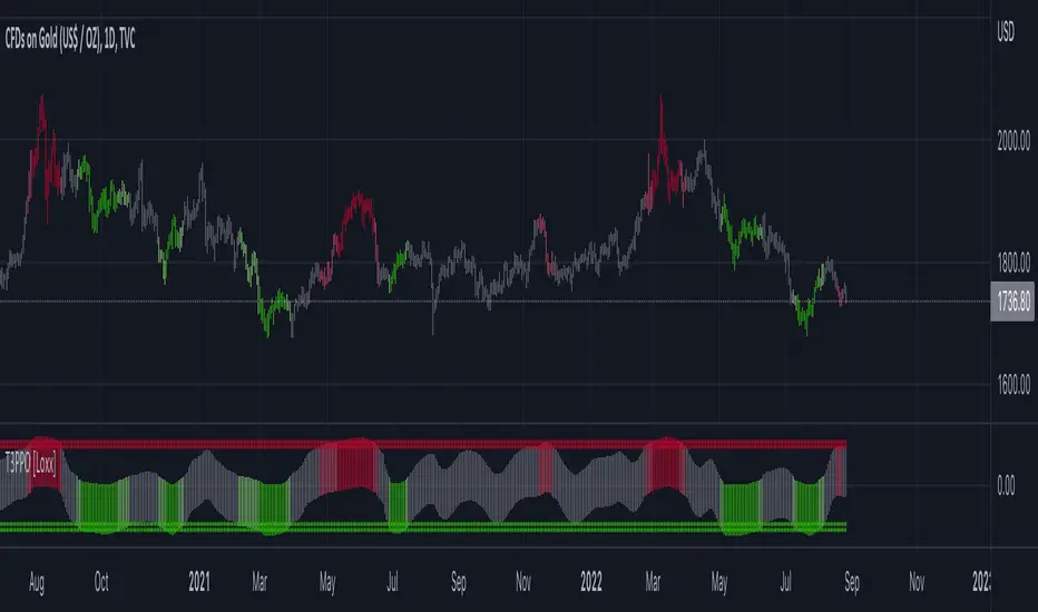
T3 PPO [Loxx]T3 PPO is a percentage price oscillator indicator using T3 moving average. This indicator is used to spot reversals. Dark red is upward price exhaustion, dark green is downward price exhaustion.
What is Percentage Price Oscillator (PPO)?
The percentage price oscillator (PPO) is a technical momentum indicator that shows the relationship between two moving averages in percentage terms. The moving averages are a 26-period and 12-period exponential moving average (EMA).
The PPO is used to compare asset performance and volatility, spot divergence that could lead to price reversals, generate trade signals, and help confirm trend direction.
What is the T3 moving average?
Better Moving Averages Tim Tillson
November 1, 1998
Tim Tillson is a software project manager at Hewlett-Packard, with degrees in Mathematics and Computer Science. He has privately traded options and equities for 15 years.
Introduction
"Digital filtering includes the process of smoothing, predicting, differentiating, integrating, separation of signals, and removal of noise from a signal. Thus many people who do such things are actually using digital filters without realizing that they are; being unacquainted with the theory, they neither understand what they have done nor the possibilities of what they might have done."
This quote from R. W. Hamming applies to the vast majority of indicators in technical analysis . Moving averages, be they simple, weighted, or exponential, are lowpass filters; low frequency components in the signal pass through with little attenuation, while high frequencies are severely reduced.
"Oscillator" type indicators (such as MACD , Momentum, Relative Strength Index ) are another type of digital filter called a differentiator.
Tushar Chande has observed that many popular oscillators are highly correlated, which is sensible because they are trying to measure the rate of change of the underlying time series, i.e., are trying to be the first and second derivatives we all learned about in Calculus.
We use moving averages (lowpass filters) in technical analysis to remove the random noise from a time series, to discern the underlying trend or to determine prices at which we will take action. A perfect moving average would have two attributes:
It would be smooth, not sensitive to random noise in the underlying time series. Another way of saying this is that its derivative would not spuriously alternate between positive and negative values.
It would not lag behind the time series it is computed from. Lag, of course, produces late buy or sell signals that kill profits.
The only way one can compute a perfect moving average is to have knowledge of the future, and if we had that, we would buy one lottery ticket a week rather than trade!
Having said this, we can still improve on the conventional simple, weighted, or exponential moving averages. Here's how:
Two Interesting Moving Averages
We will examine two benchmark moving averages based on Linear Regression analysis.
In both cases, a Linear Regression line of length n is fitted to price data.
I call the first moving average ILRS, which stands for Integral of Linear Regression Slope. One simply integrates the slope of a linear regression line as it is successively fitted in a moving window of length n across the data, with the constant of integration being a simple moving average of the first n points. Put another way, the derivative of ILRS is the linear regression slope. Note that ILRS is not the same as a SMA ( simple moving average ) of length n, which is actually the midpoint of the linear regression line as it moves across the data.
We can measure the lag of moving averages with respect to a linear trend by computing how they behave when the input is a line with unit slope. Both SMA (n) and ILRS(n) have lag of n/2, but ILRS is much smoother than SMA .
Our second benchmark moving average is well known, called EPMA or End Point Moving Average. It is the endpoint of the linear regression line of length n as it is fitted across the data. EPMA hugs the data more closely than a simple or exponential moving average of the same length. The price we pay for this is that it is much noisier (less smooth) than ILRS, and it also has the annoying property that it overshoots the data when linear trends are present.
However, EPMA has a lag of 0 with respect to linear input! This makes sense because a linear regression line will fit linear input perfectly, and the endpoint of the LR line will be on the input line.
These two moving averages frame the tradeoffs that we are facing. On one extreme we have ILRS, which is very smooth and has considerable phase lag. EPMA has 0 phase lag, but is too noisy and overshoots. We would like to construct a better moving average which is as smooth as ILRS, but runs closer to where EPMA lies, without the overshoot.
A easy way to attempt this is to split the difference, i.e. use (ILRS(n)+EPMA(n))/2. This will give us a moving average (call it IE /2) which runs in between the two, has phase lag of n/4 but still inherits considerable noise from EPMA. IE /2 is inspirational, however. Can we build something that is comparable, but smoother? Figure 1 shows ILRS, EPMA, and IE /2.
Filter Techniques
Any thoughtful student of filter theory (or resolute experimenter) will have noticed that you can improve the smoothness of a filter by running it through itself multiple times, at the cost of increasing phase lag.
There is a complementary technique (called twicing by J.W. Tukey) which can be used to improve phase lag. If L stands for the operation of running data through a low pass filter, then twicing can be described by:
L' = L(time series) + L(time series - L(time series))
That is, we add a moving average of the difference between the input and the moving average to the moving average. This is algebraically equivalent to:
2L-L(L)
This is the Double Exponential Moving Average or DEMA , popularized by Patrick Mulloy in TASAC (January/February 1994).
In our taxonomy, DEMA has some phase lag (although it exponentially approaches 0) and is somewhat noisy, comparable to IE /2 indicator.
We will use these two techniques to construct our better moving average, after we explore the first one a little more closely.
Fixing Overshoot
An n-day EMA has smoothing constant alpha=2/(n+1) and a lag of (n-1)/2.
Thus EMA (3) has lag 1, and EMA (11) has lag 5. Figure 2 shows that, if I am willing to incur 5 days of lag, I get a smoother moving average if I run EMA (3) through itself 5 times than if I just take EMA (11) once.
This suggests that if EPMA and DEMA have 0 or low lag, why not run fast versions (eg DEMA (3)) through themselves many times to achieve a smooth result? The problem is that multiple runs though these filters increase their tendency to overshoot the data, giving an unusable result. This is because the amplitude response of DEMA and EPMA is greater than 1 at certain frequencies, giving a gain of much greater than 1 at these frequencies when run though themselves multiple times. Figure 3 shows DEMA (7) and EPMA(7) run through themselves 3 times. DEMA^3 has serious overshoot, and EPMA^3 is terrible.
The solution to the overshoot problem is to recall what we are doing with twicing:
DEMA (n) = EMA (n) + EMA (time series - EMA (n))
The second term is adding, in effect, a smooth version of the derivative to the EMA to achieve DEMA . The derivative term determines how hot the moving average's response to linear trends will be. We need to simply turn down the volume to achieve our basic building block:
EMA (n) + EMA (time series - EMA (n))*.7;
This is algebraically the same as:
EMA (n)*1.7-EMA( EMA (n))*.7;
I have chosen .7 as my volume factor, but the general formula (which I call "Generalized Dema") is:
GD (n,v) = EMA (n)*(1+v)-EMA( EMA (n))*v,
Where v ranges between 0 and 1. When v=0, GD is just an EMA , and when v=1, GD is DEMA . In between, GD is a cooler DEMA . By using a value for v less than 1 (I like .7), we cure the multiple DEMA overshoot problem, at the cost of accepting some additional phase delay. Now we can run GD through itself multiple times to define a new, smoother moving average T3 that does not overshoot the data:
T3(n) = GD ( GD ( GD (n)))
In filter theory parlance, T3 is a six-pole non-linear Kalman filter. Kalman filters are ones which use the error (in this case (time series - EMA (n)) to correct themselves. In Technical Analysis , these are called Adaptive Moving Averages; they track the time series more aggressively when it is making large moves.
CT Moving Average Crossover IndicatorMoving Average Crossover Indicator
Here I present a moving average indicator with 9 user definable moving averages from which up to 5 pairs can be selected to show what prices would need to be closed at on the current bar to cross each individual pair.
I have put much emphasis here on simplicity of setting the parameters of the moving averages, selecting the crossover pairs and on the clarity of the displayed information in the optional “Moving Average Crossover Level” Information Box.
What Is a Moving Average (MA)?
According to Investopedia - “In statistics, a moving average is a calculation used to analyze data points by creating a series of averages of different subsets of the full data set.
In finance, a moving average (MA) is a stock indicator that is commonly used in technical analysis. The reason for calculating the moving average of a stock is to help smooth out the price data by creating a constantly updated average price.
By calculating the moving average, the impacts of random, short-term fluctuations on the price of a stock over a specified time-frame are mitigated.”
The user can set the color, type (SMA/EMA) and length of each of the 9 moving averages.
Then the user may choose 5 pairs of moving averages from the set of 9.
The script will then calculate the price needed to be crossed by the close of the current bar in order to crossover each of the user defined pairs and outputs the results as optional lineplots and/or an Infobox which shows the relevant information in a very clear way.
The user may switch the moving averages, crossover lineplots and infobox on and off easily with one click boxes in the settings menu.
The number of decimal places shown in the Infobox can be altered in the settings menu.
If the price required to cross a pair of moving averages is zero or less, the crossover level will display “Impossible” and the plots will plot at zero. (this helps ameliorate chart auto-focus issues)
Quoting a variety of online resources …….
Understanding Moving Averages (MA)
Moving averages are a simple, technical analysis tool. Moving averages are usually calculated to identify the trend direction of a stock or to determine its support and resistance levels. It is a trend-following—or lagging—indicator because it is based on past prices.
The longer the time period for the moving average, the greater the lag. So, a 200-day moving average will have a much greater degree of lag than a 20-day MA because it contains prices for the past 200 days. The 50-day and 200-day moving average figures for stocks are widely followed by investors and traders and are considered to be important trading signals.
Moving averages are a totally customizable indicator, which means that an investor can freely choose whatever time frame they want when calculating an average. The most common time periods used in moving averages are 15, 20, 30, 50, 100, and 200 days. The shorter the time span used to create the average, the more sensitive it will be to price changes. The longer the time span, the less sensitive the average will be.
Investors may choose different time periods of varying lengths to calculate moving averages based on their trading objectives. Shorter moving averages are typically used for short-term trading, while longer-term moving averages are more suited for long-term investors.
There is no correct time frame to use when setting up your moving averages. The best way to figure out which one works best for you is to experiment with a number of different time periods until you find one that fits your strategy.
Predicting trends in the stock market is no simple process. While it is impossible to predict the future movement of a specific stock, using technical analysis and research can help you make better predictions.
A rising moving average indicates that the security is in an uptrend, while a declining moving average indicates that it is in a downtrend. Similarly, upward momentum is confirmed with a bullish crossover, which occurs when a short-term moving average crosses above a longer-term moving average. Conversely, downward momentum is confirmed with a bearish crossover, which occurs when a short-term moving average crosses below a longer-term moving average.
Types of Moving Averages
Simple Moving Average (SMA)
The simplest form of a moving average, known as a simple moving average (SMA), is calculated by taking the arithmetic mean of a given set of values. In other words, a set of numbers–or prices in the case of financial instruments–are added together and then divided by the number of prices in the set.
Exponential Moving Average (EMA)
The exponential moving average is a type of moving average that gives more weight to recent prices in an attempt to make it more responsive to new information.
To calculate an EMA, you must first compute the simple moving average (SMA) over a particular time period. Next, you must calculate the multiplier for weighting the EMA (referred to as the "smoothing factor"), which typically follows the formula: 2/(selected time period + 1). So, for a 20-day moving average, the multiplier would be 2/(20+1)= 0.0952. Then you use the smoothing factor combined with the previous EMA to arrive at the current value.
The EMA thus gives a higher weighting to recent prices, while the SMA assigns equal weighting to all values.

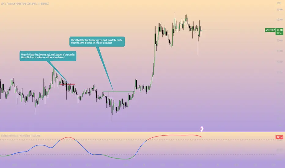
Hull Suite Oscillator - Normalized | IkkeOmarThis script is based off the Hull Suite by @InSilico.
I made this script to provide and calculate the Hull Moving Average (HMA) based on the chosen variation (HMA, TMA, or EMA) and length to then normalize the HMA values to a range of 0 to 100. The normalized values are further smoothed using an exponential moving average (EMA).
The smoothed oscillator is plotted as a line, where values above 80 are colored red, values below 20 are colored green, and values between 20 and 80 are colored blue. Additionally, there are horizontal dashed lines at the levels of 20 and 80 to serve as reference points.
Explanation for the code:
The script uses the close price of the asset as the source for calculations. The modeSwitch parameter allows selecting the type of Hull variation: Hma, Thma, or Ehma. The length parameter determines the calculation period for the Hull moving averages. The lengthMult parameter is used to adjust the length for higher timeframes. The oscSmooth parameter determines the lookback period for smoothing the oscillator.
There are three functions defined for calculating different types of Hull moving averages: HMA, EHMA, and THMA. These functions take the source and length as inputs and return the corresponding Hull moving average.
The Mode function acts as a switch and selects the appropriate Hull variation based on the modeSwitch parameter. It returns the chosen Hull moving average.
The script calculates the Hull moving averages using the selected mode, source, and length. The main Hull moving average is stored in the _hull variable, and aliases are created for the main Hull moving average (HULL), the main Hull value (MHULL), and the secondary Hull value (SHULL).
To create the normalized oscillator values, the script finds the highest and lowest values of the Hull moving average within the specified length. It then normalizes the Hull values to a range of 0 to 100 using a formula. This normalized oscillator represents the strength of the trend.
To smooth out the oscillator values, an exponential moving average is applied using the oscSmooth parameter.
The smoothed oscillator is plotted as a line chart. The line color is determined based on the oscillator value using conditional statements. If the oscillator value is above or equal to 80, the line color is set to red. If it is below or equal to 20, the color is green. Otherwise, it is blue. The linewidth is set to 2.
Additionally, two horizontal reference lines are plotted at levels 20 and 80 for visual reference. They are displayed in gray and dashed style.
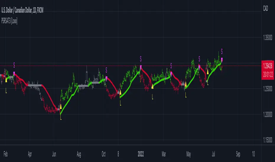
Pips-Stepped, R-squared Adaptive T3 [Loxx]Pips-Stepped, R-squared Adaptive T3 is a a T3 moving average with optional adaptivity, trend following, and pip-stepping. This indicator also uses optional flat coloring to determine chops zones. This indicator is R-squared adaptive. This is also an experimental indicator.
What is the T3 moving average?
Better Moving Averages Tim Tillson
November 1, 1998
Tim Tillson is a software project manager at Hewlett-Packard, with degrees in Mathematics and Computer Science. He has privately traded options and equities for 15 years.
Introduction
"Digital filtering includes the process of smoothing, predicting, differentiating, integrating, separation of signals, and removal of noise from a signal. Thus many people who do such things are actually using digital filters without realizing that they are; being unacquainted with the theory, they neither understand what they have done nor the possibilities of what they might have done."
This quote from R. W. Hamming applies to the vast majority of indicators in technical analysis . Moving averages, be they simple, weighted, or exponential, are lowpass filters; low frequency components in the signal pass through with little attenuation, while high frequencies are severely reduced.
"Oscillator" type indicators (such as MACD , Momentum, Relative Strength Index ) are another type of digital filter called a differentiator.
Tushar Chande has observed that many popular oscillators are highly correlated, which is sensible because they are trying to measure the rate of change of the underlying time series, i.e., are trying to be the first and second derivatives we all learned about in Calculus.
We use moving averages (lowpass filters) in technical analysis to remove the random noise from a time series, to discern the underlying trend or to determine prices at which we will take action. A perfect moving average would have two attributes:
It would be smooth, not sensitive to random noise in the underlying time series. Another way of saying this is that its derivative would not spuriously alternate between positive and negative values.
It would not lag behind the time series it is computed from. Lag, of course, produces late buy or sell signals that kill profits.
The only way one can compute a perfect moving average is to have knowledge of the future, and if we had that, we would buy one lottery ticket a week rather than trade!
Having said this, we can still improve on the conventional simple, weighted, or exponential moving averages. Here's how:
Two Interesting Moving Averages
We will examine two benchmark moving averages based on Linear Regression analysis.
In both cases, a Linear Regression line of length n is fitted to price data.
I call the first moving average ILRS, which stands for Integral of Linear Regression Slope. One simply integrates the slope of a linear regression line as it is successively fitted in a moving window of length n across the data, with the constant of integration being a simple moving average of the first n points. Put another way, the derivative of ILRS is the linear regression slope. Note that ILRS is not the same as a SMA ( simple moving average ) of length n, which is actually the midpoint of the linear regression line as it moves across the data.
We can measure the lag of moving averages with respect to a linear trend by computing how they behave when the input is a line with unit slope. Both SMA (n) and ILRS(n) have lag of n/2, but ILRS is much smoother than SMA .
Our second benchmark moving average is well known, called EPMA or End Point Moving Average. It is the endpoint of the linear regression line of length n as it is fitted across the data. EPMA hugs the data more closely than a simple or exponential moving average of the same length. The price we pay for this is that it is much noisier (less smooth) than ILRS, and it also has the annoying property that it overshoots the data when linear trends are present.
However, EPMA has a lag of 0 with respect to linear input! This makes sense because a linear regression line will fit linear input perfectly, and the endpoint of the LR line will be on the input line.
These two moving averages frame the tradeoffs that we are facing. On one extreme we have ILRS, which is very smooth and has considerable phase lag. EPMA has 0 phase lag, but is too noisy and overshoots. We would like to construct a better moving average which is as smooth as ILRS, but runs closer to where EPMA lies, without the overshoot.
A easy way to attempt this is to split the difference, i.e. use (ILRS(n)+EPMA(n))/2. This will give us a moving average (call it IE /2) which runs in between the two, has phase lag of n/4 but still inherits considerable noise from EPMA. IE /2 is inspirational, however. Can we build something that is comparable, but smoother? Figure 1 shows ILRS, EPMA, and IE /2.
Filter Techniques
Any thoughtful student of filter theory (or resolute experimenter) will have noticed that you can improve the smoothness of a filter by running it through itself multiple times, at the cost of increasing phase lag.
There is a complementary technique (called twicing by J.W. Tukey) which can be used to improve phase lag. If L stands for the operation of running data through a low pass filter, then twicing can be described by:
L' = L(time series) + L(time series - L(time series))
That is, we add a moving average of the difference between the input and the moving average to the moving average. This is algebraically equivalent to:
2L-L(L)
This is the Double Exponential Moving Average or DEMA , popularized by Patrick Mulloy in TASAC (January/February 1994).
In our taxonomy, DEMA has some phase lag (although it exponentially approaches 0) and is somewhat noisy, comparable to IE /2 indicator.
We will use these two techniques to construct our better moving average, after we explore the first one a little more closely.
Fixing Overshoot
An n-day EMA has smoothing constant alpha=2/(n+1) and a lag of (n-1)/2.
Thus EMA (3) has lag 1, and EMA (11) has lag 5. Figure 2 shows that, if I am willing to incur 5 days of lag, I get a smoother moving average if I run EMA (3) through itself 5 times than if I just take EMA (11) once.
This suggests that if EPMA and DEMA have 0 or low lag, why not run fast versions (eg DEMA (3)) through themselves many times to achieve a smooth result? The problem is that multiple runs though these filters increase their tendency to overshoot the data, giving an unusable result. This is because the amplitude response of DEMA and EPMA is greater than 1 at certain frequencies, giving a gain of much greater than 1 at these frequencies when run though themselves multiple times. Figure 3 shows DEMA (7) and EPMA(7) run through themselves 3 times. DEMA^3 has serious overshoot, and EPMA^3 is terrible.
The solution to the overshoot problem is to recall what we are doing with twicing:
DEMA (n) = EMA (n) + EMA (time series - EMA (n))
The second term is adding, in effect, a smooth version of the derivative to the EMA to achieve DEMA . The derivative term determines how hot the moving average's response to linear trends will be. We need to simply turn down the volume to achieve our basic building block:
EMA (n) + EMA (time series - EMA (n))*.7;
This is algebraically the same as:
EMA (n)*1.7-EMA( EMA (n))*.7;
I have chosen .7 as my volume factor, but the general formula (which I call "Generalized Dema") is:
GD (n,v) = EMA (n)*(1+v)-EMA( EMA (n))*v,
Where v ranges between 0 and 1. When v=0, GD is just an EMA , and when v=1, GD is DEMA . In between, GD is a cooler DEMA . By using a value for v less than 1 (I like .7), we cure the multiple DEMA overshoot problem, at the cost of accepting some additional phase delay. Now we can run GD through itself multiple times to define a new, smoother moving average T3 that does not overshoot the data:
T3(n) = GD ( GD ( GD (n)))
In filter theory parlance, T3 is a six-pole non-linear Kalman filter. Kalman filters are ones which use the error (in this case (time series - EMA (n)) to correct themselves. In Technical Analysis , these are called Adaptive Moving Averages; they track the time series more aggressively when it is making large moves.
What is R-squared Adaptive?
One tool available in forecasting the trendiness of the breakout is the coefficient of determination (R-squared), a statistical measurement.
The R-squared indicates linear strength between the security's price (the Y - axis) and time (the X - axis). The R-squared is the percentage of squared error that the linear regression can eliminate if it were used as the predictor instead of the mean value. If the R-squared were 0.99, then the linear regression would eliminate 99% of the error for prediction versus predicting closing prices using a simple moving average.
R-squared is used here to derive a T3 factor used to modify price before passing price through a six-pole non-linear Kalman filter.
Included:
Bar coloring
Signals
Alerts
Flat coloring
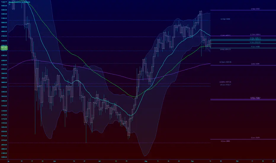
Overlay Indicators (EMAs, SMAs, Ichimoku & Bollinger Bands)This is a combination of popular overlay indicators that are used for dynamic support and resistance, trade targets and trend strength.
Included are:
-> 6 Exponential Moving Averages
-> 6 Simple Moving Averages
-> Ichimoku Cloud
-> Bollinger Bands
-> There is also a weekend background marker ideal for cryptocurrency trading
Using all these indicators in conjunction with each other provide great confluence and confidence in trades and price targets.
An explanation of each indicator is listed below.
What Is an Exponential Moving Average (EMA)?
"An exponential moving average (EMA) is a type of moving average (MA) that places a greater weight and significance on the most recent data points. The exponential moving average is also referred to as the exponentially weighted moving average. An exponentially weighted moving average reacts more significantly to recent price changes than a simple moving average (SMA), which applies an equal weight to all observations in the period.
What Does the Exponential Moving Average Tell You?
The 12- and 26-day exponential moving averages (EMAs) are often the most quoted and analyzed short-term averages. The 12- and 26-day are used to create indicators like the moving average convergence divergence (MACD) and the percentage price oscillator (PPO). In general, the 50- and 200-day EMAs are used as indicators for long-term trends. When a stock price crosses its 200-day moving average, it is a technical signal that a reversal has occurred.
Traders who employ technical analysis find moving averages very useful and insightful when applied correctly. However, they also realize that these signals can create havoc when used improperly or misinterpreted. All the moving averages commonly used in technical analysis are, by their very nature, lagging indicators."
Source: www.investopedia.com
Popular EMA lookback periods include fibonacci numbers and round numbers such as the 100 or 200. The default values of the EMAs in this indicator are the most widely used, specifically for cryptocurrency but they also work very well with traditional.
EMAs are normally used in conjunction with Simple Moving Averages.
" What Is Simple Moving Average (SMA)?
A simple moving average (SMA) calculates the average of a selected range of prices, usually closing prices, by the number of periods in that range.
Simple Moving Average vs. Exponential Moving Average
The major difference between an exponential moving average (EMA) and a simple moving average is the sensitivity each one shows to changes in the data used in its calculation. More specifically, the EMA gives a higher weighting to recent prices, while the SMA assigns an equal weighting to all values."
Source: www.investopedia.com
In this indicator, I've included 6 popular moving averages that are commonly used. Most traders will find specific settings for their own personal trading style.
Along with the EMA and SMA, another indicator that is good for finding confluence between these two is the Ichimoku Cloud.
" What is the Ichimoku Cloud?
The Ichimoku Cloud is a collection of technical indicators that show support and resistance levels, as well as momentum and trend direction. It does this by taking multiple averages and plotting them on the chart. It also uses these figures to compute a "cloud" which attempts to forecast where the price may find support or resistance in the future.
The Ichimoku cloud was developed by Goichi Hosoda, a Japanese journalist, and published in the late 1960s.1 It provides more data points than the standard candlestick chart. While it seems complicated at first glance, those familiar with how to read the charts often find it easy to understand with well-defined trading signals."
More info can be seen here: www.investopedia.com
I have changed the default settings on the Ichimoku to suit cryptocurrency trading (as cryptocurrency is usually fast and thus require slightly longer lookbacks) to 20 60 120 30.
Along with the Ichimoku, I like to use Bollinger Bands to not only find confluence for support and resistance but for price discovery targets and trend strength.
" What Is a Bollinger Band®?
A Bollinger Band® is a technical analysis tool defined by a set of trendlines plotted two standard deviations (positively and negatively) away from a simple moving average (SMA) of a security's price, but which can be adjusted to user preferences.
Bollinger Bands® were developed and copyrighted by famous technical trader John Bollinger, designed to discover opportunities that give investors a higher probability of properly identifying when an asset is oversold or overbought."
This article goes into great detail of the complexities of using the Bollinger band and how to use it.
=======
This indicator combines all these powerful indicators into one so that it is easier to input different settings, turn specific tools on or off and can be easily customised.
MechArt Moving Average and % Above V1.1MechArt Moving Average and % Above V1.1
Unlock the power of custom analysis with this Adjustable Moving Average Indicator! Whether you're a day trader, swing trader, or long-term investor, this tool helps you track price action with precision and flexibility. Tailor your trading strategy to your needs by adjusting the type of moving average, price triggers, and percentage levels.
🔑 Key Features:
Choose Your Moving Average Type 🌀
Select from four popular moving averages:
SMA (Simple Moving Average)
EMA (Exponential Moving Average)
WMA (Weighted Moving Average)
VWMA (Volume Weighted Moving Average)
Find the one that best fits your trading style!
Adjustable Trigger Price
Choose between four price types to trigger signals:
Open
High
Low
Close
Pick the price type that makes the most sense for your strategy!
Percentage Above the Moving Average 📈🔽
Set a custom percentage above the moving average to generate alerts when the price reaches key levels.
Customizable Alerts 🔔
Get notified when the price is above the target price or below the moving average. Perfect for timely trades!
📉 Visual Alerts:
🔴 Red Background: When the selected price is above the target price (percentage above the moving average).
🟩 Green Background: When the selected price is below the moving average.
🚀 How This Indicator Helps You:
Precision 🎯: Visual signals with clear red and green backgrounds help you make quick decisions based on the price's relationship to your moving average.
Flexibility 🔄: Customize the type of moving average and the price used for triggers to fit your trading style.
📊 Perfect For:
Swing Traders 📈: Use the indicator to identify price trends and reversals based on moving averages.
Day Traders ⏳: Set short-term percentage levels to catch immediate price movements.
Long-Term Investors 💼: Track longer-term trends and set alerts when prices deviate significantly from your moving average.
Take control of your trading strategy with this Adjustable Moving Average Indicator and start making more informed decisions today! 🏅
Change from V1.0: Fixed Timeframe setting to match chart.

MechArt Moving Average and % Above V1.0MechArt Moving Average and % Above V1.0
Unlock the power of custom analysis with this Adjustable Moving Average Indicator! Whether you're a day trader, swing trader, or long-term investor, this tool helps you track price action with precision and flexibility. Tailor your trading strategy to your needs by adjusting the type of moving average, price triggers, and percentage levels.
🔑 Key Features:
Choose Your Moving Average Type 🌀
Select from four popular moving averages:
SMA (Simple Moving Average)
EMA (Exponential Moving Average)
WMA (Weighted Moving Average)
VWMA (Volume Weighted Moving Average)
Find the one that best fits your trading style!
Adjustable Trigger Price
Choose between four price types to trigger signals:
Open
High
Low
Close
Pick the price type that makes the most sense for your strategy!
Percentage Above the Moving Average 📈🔽
Set a custom percentage above the moving average to generate alerts when the price reaches key levels.
Customizable Alerts 🔔
Get notified when the price is above the target price or below the moving average. Perfect for timely trades!
📉 Visual Alerts:
🔴 Red Background: When the selected price is above the target price (percentage above the moving average).
🟩 Green Background: When the selected price is below the moving average.
📅 Adjustable Timeframe:
Choose the timeframe that suits you! Whether you're trading on a 1-minute chart, 1-hour, 1-day, or 1-week, this indicator works for all timeframes.
🚀 How This Indicator Helps You:
Precision 🎯: Visual signals with clear red and green backgrounds help you make quick decisions based on the price's relationship to your moving average.
Flexibility 🔄: Customize the type of moving average and the price used for triggers to fit your trading style.
📊 Perfect For:
Swing Traders 📈: Use the indicator to identify price trends and reversals based on moving averages.
Day Traders ⏳: Set short-term percentage levels to catch immediate price movements.
Long-Term Investors 💼: Track longer-term trends and set alerts when prices deviate significantly from your moving average.
Take control of your trading strategy with this Adjustable Moving Average Indicator and start making more informed decisions today! 🏅

Alxuse Supertrend 4EMA Buy and Sell for tutorialAll abilities of Supertrend, moreover :
Drawing 4 EMA band & the ability to change values, change colors, turn on/off show.
Sends Signal Sell and Buy in multi timeframe.
The ability used in the alert section and create customized alerts.
To receive valid alerts the replay section , the timeframe of the chart must be the same as the timeframe of the indicator.
Supertrend with a simple EMA Filter can improve the performance of the signals during a strong trend.
For detecting the continuation of the downward and upward trend we can use 4 EMA colors.
In the upward trend , the EMA lines are in order of green, blue, red, yellow from bottom to top.
In the downward trend, the EMA lines are in order of yellow, red, blue, green from bottom to top.
How it works:
x1 = MA1 < MA2 and MA2 < MA3 and MA3 < MA4 and ta.crossunder(MA3, MA4)
x2 = MA1 < MA2 and MA2 < MA3 and MA3 < MA4 and ta.crossunder(MA2, MA3)
x3 = MA1 < MA2 and MA2 < MA3 and MA3 < MA4 and ta.crossunder(MA1, MA2)
y1 = MA4 < MA3 and MA3 < MA2 and MA2 < MA1 and ta.crossover(MA3, MA4)
y2 = MA4 < MA3 and MA3 < MA2 and MA2 < MA1 and ta.crossover(MA2, MA3)
y3 = MA4 < MA3 and MA3 < MA2 and MA2 < MA1 and ta.crossover(MA1, MA2)
Red triangle = x1 or x2 or x3
Green triangle = y1 or y2 or y3
Long = BUY signal and followed by a Green triangle
Exit Long = SELL signal
Short = SELL signal and followed by a Red triangle
Exit Short = BUY signal
It is also possible to get help from the Stochastic RSI and MACD indicators for confirmation.
For receiving a signal with these two conditions or more conditions, i am making a video tutorial that I will release soon.
Supertrend
Definition
Supertrend is a trend-following indicator based on Average True Range (ATR). The calculation of its single line combines trend detection and volatility. It can be used to detect changes in trend direction and to position stops.
The basics
The Supertrend is a trend-following indicator. It is overlaid on the main chart and their plots indicate the current trend. A Supertrend can be used with varying periods (daily, weekly, intraday etc.) and on varying instruments.
The Supertrend has several inputs that you can adjust to match your trading strategy. Adjusting these settings allows you to make the indicator more or less sensitive to price changes.
For the Supertrend inputs, you can adjust atrLength and multiplier:
the atrLength setting is the lookback length for the ATR calculation;
multiplier is what the ATR is multiplied by to offset the bands from price.
When the price falls below the indicator curve, it turns red and indicates a downtrend. Conversely, when the price rises above the curve, the indicator turns green and indicates an uptrend. After each close above or below Supertrend, a new trend appears.
Summary
The Supertrend helps you make the right trading decisions. However, there are times when it generates false signals. Therefore, it is best to use the right combination of several indicators. Like any other indicator, Supertrend works best when used with other indicators such as MACD, Parabolic SAR, or RSI.
Exponential Moving Average
Definition
The Exponential Moving Average (EMA) is a specific type of moving average that points towards the importance of the most recent data and information from the market. The Exponential Moving Average is just like it’s name says - it’s exponential, weighting the most recent prices more than the less recent prices. The EMA can be compared and contrasted with the simple moving average.
Similar to other moving averages, the EMA is a technical indicator that produces buy and sell signals based on data that shows evidence of divergence and crossovers from general and historical averages. Additionally, the EMA tries to amplify the importance that the most recent data points play in a calculation.
It is common to use more than one EMA length at once, to provide more in-depth and focused data. For example, by choosing 10-day and 200-day moving averages, a trader is able to determine more from the results in a long-term trade, than a trader who is only analyzing one EMA length.
It’s best to use the EMA when for trending markets, as it shows uptrends and downtrends when a market is strong and weak, respectively. An experienced trader will know to look both at the line the EMA projects, as well as the rate of change that comes from each bar as it moves to the next data point. Analyzing these points and data streams correctly will help the trader determine when they should buy, sell, or switch investments from bearish to bullish or vice versa.
Short-term averages, on the other hand, is a different story when analyzing Exponential Moving Average data. It is most common for traders to quote and utilize 12- and 26-day EMAs in the short-term. This is because they are used to create specific indicators. Look into Moving Average Convergence Divergence (MACD) for more information. Similarly, the 50- and 200-day moving averages are most common for analyzing long-term trends.
Moving averages can be very useful for traders using technical analysis for profit. It is important to identify and realize, however, their shortcomings, as all moving averages tend to suffer from recurring lag. It is difficult to modify the moving average to work in your favor at times, often having the preferred time to enter or exit the market pass before the moving average even shows changes in the trend or price movement for that matter.
All of this is true, however, the EMA strives to make this easier for traders. The EMA is unique because it places more emphasis on the most recent data. Therefore, price movement and trend reversals or changes are closely monitored, allowing for the EMA to react quicker than other moving averages.
Limitations
Although using the Exponential Moving Average has a lot of advantages when analyzing market trends, it is also uncertain whether or not the use of most recent data points truly affects technical and market analysis. In addition, the EMA relies on historical data as its basis for operating and because news, events, and other information can change rapidly the indicator can misinterpret this information by weighting the current prices higher than when the event actually occurred.
Summary
The Exponential Moving Average (EMA) is a moving average and technical indicator that reflects and projects the most recent data and information from the market to a trader and relies on a base of historical data. It is one of many different types of moving averages and has an easily calculable formula.
The added features to the indicator are made for training, it is advisable to use it with caution in tradings.

Extended Moving Average (MA) LibraryThis Extended Moving Average Library is a sophisticated and comprehensive tool for traders seeking to expand their arsenal of moving averages for more nuanced and detailed technical analysis.
The library contains various types of moving averages, each with two versions - one that accepts a simple constant length parameter and another that accepts a series or changing length parameter.
This makes the library highly versatile and suitable for a wide range of strategies and trading styles.
Moving Averages Included:
Simple Moving Average (SMA): This is the most basic type of moving average. It calculates the average of a selected range of prices, typically closing prices, by the number of periods in that range.
Exponential Moving Average (EMA): This type of moving average gives more weight to the latest data and is thus more responsive to new price information. This can help traders to react faster to recent price changes.
Double Exponential Moving Average (DEMA): This is a composite of a single exponential moving average, a double exponential moving average, and an exponential moving average of a triple exponential moving average. It aims to eliminate lag, which is a key drawback of using moving averages.
Jurik Moving Average (JMA): This is a versatile and responsive moving average that can be adjusted for market speed. It is designed to stay balanced and responsive, regardless of how long or short it is.
Kaufman's Adaptive Moving Average (KAMA): This moving average is designed to account for market noise or volatility. KAMA will closely follow prices when the price swings are relatively small and the noise is low.
Smoothed Moving Average (SMMA): This type of moving average applies equal weighting to all observations and smooths out the data.
Triangular Moving Average (TMA): This is a double smoothed simple moving average, calculated by averaging the simple moving averages of a dataset.
True Strength Force (TSF): This is a moving average of the linear regression line, a statistical tool used to predict future values from past values.
Volume Moving Average (VMA): This is a simple moving average of a volume, which can help to identify trends in volume.
Volume Adjusted Moving Average (VAMA): This moving average adjusts for volume and can be more responsive to volume changes.
Zero Lag Exponential Moving Average (ZLEMA): This type of moving average aims to eliminate the lag in traditional EMAs, making it more responsive to recent price changes.
Selector: The selector function allows users to easily select and apply any of the moving averages included in the library inside their strategy.
This library provides a broad selection of moving averages to choose from, allowing you to experiment with different types and find the one that best suits your trading strategy.
By providing both simple and series versions for each moving average, this library offers great flexibility, enabling users to pass both constant and changing length parameters as needed.

STD-Adaptive T3 [Loxx]STD-Adaptive T3 is a standard deviation adaptive T3 moving average filter. This indicator acts more like a trend overlay indicator with gradient coloring.
What is the T3 moving average?
Better Moving Averages Tim Tillson
November 1, 1998
Tim Tillson is a software project manager at Hewlett-Packard, with degrees in Mathematics and Computer Science. He has privately traded options and equities for 15 years.
Introduction
"Digital filtering includes the process of smoothing, predicting, differentiating, integrating, separation of signals, and removal of noise from a signal. Thus many people who do such things are actually using digital filters without realizing that they are; being unacquainted with the theory, they neither understand what they have done nor the possibilities of what they might have done."
This quote from R. W. Hamming applies to the vast majority of indicators in technical analysis . Moving averages, be they simple, weighted, or exponential, are lowpass filters; low frequency components in the signal pass through with little attenuation, while high frequencies are severely reduced.
"Oscillator" type indicators (such as MACD , Momentum, Relative Strength Index ) are another type of digital filter called a differentiator.
Tushar Chande has observed that many popular oscillators are highly correlated, which is sensible because they are trying to measure the rate of change of the underlying time series, i.e., are trying to be the first and second derivatives we all learned about in Calculus.
We use moving averages (lowpass filters) in technical analysis to remove the random noise from a time series, to discern the underlying trend or to determine prices at which we will take action. A perfect moving average would have two attributes:
It would be smooth, not sensitive to random noise in the underlying time series. Another way of saying this is that its derivative would not spuriously alternate between positive and negative values.
It would not lag behind the time series it is computed from. Lag, of course, produces late buy or sell signals that kill profits.
The only way one can compute a perfect moving average is to have knowledge of the future, and if we had that, we would buy one lottery ticket a week rather than trade!
Having said this, we can still improve on the conventional simple, weighted, or exponential moving averages. Here's how:
Two Interesting Moving Averages
We will examine two benchmark moving averages based on Linear Regression analysis.
In both cases, a Linear Regression line of length n is fitted to price data.
I call the first moving average ILRS, which stands for Integral of Linear Regression Slope. One simply integrates the slope of a linear regression line as it is successively fitted in a moving window of length n across the data, with the constant of integration being a simple moving average of the first n points. Put another way, the derivative of ILRS is the linear regression slope. Note that ILRS is not the same as a SMA ( simple moving average ) of length n, which is actually the midpoint of the linear regression line as it moves across the data.
We can measure the lag of moving averages with respect to a linear trend by computing how they behave when the input is a line with unit slope. Both SMA (n) and ILRS(n) have lag of n/2, but ILRS is much smoother than SMA .
Our second benchmark moving average is well known, called EPMA or End Point Moving Average. It is the endpoint of the linear regression line of length n as it is fitted across the data. EPMA hugs the data more closely than a simple or exponential moving average of the same length. The price we pay for this is that it is much noisier (less smooth) than ILRS, and it also has the annoying property that it overshoots the data when linear trends are present.
However, EPMA has a lag of 0 with respect to linear input! This makes sense because a linear regression line will fit linear input perfectly, and the endpoint of the LR line will be on the input line.
These two moving averages frame the tradeoffs that we are facing. On one extreme we have ILRS, which is very smooth and has considerable phase lag. EPMA has 0 phase lag, but is too noisy and overshoots. We would like to construct a better moving average which is as smooth as ILRS, but runs closer to where EPMA lies, without the overshoot.
A easy way to attempt this is to split the difference, i.e. use (ILRS(n)+EPMA(n))/2. This will give us a moving average (call it IE /2) which runs in between the two, has phase lag of n/4 but still inherits considerable noise from EPMA. IE /2 is inspirational, however. Can we build something that is comparable, but smoother? Figure 1 shows ILRS, EPMA, and IE /2.
Filter Techniques
Any thoughtful student of filter theory (or resolute experimenter) will have noticed that you can improve the smoothness of a filter by running it through itself multiple times, at the cost of increasing phase lag.
There is a complementary technique (called twicing by J.W. Tukey) which can be used to improve phase lag. If L stands for the operation of running data through a low pass filter, then twicing can be described by:
L' = L(time series) + L(time series - L(time series))
That is, we add a moving average of the difference between the input and the moving average to the moving average. This is algebraically equivalent to:
2L-L(L)
This is the Double Exponential Moving Average or DEMA , popularized by Patrick Mulloy in TASAC (January/February 1994).
In our taxonomy, DEMA has some phase lag (although it exponentially approaches 0) and is somewhat noisy, comparable to IE /2 indicator.
We will use these two techniques to construct our better moving average, after we explore the first one a little more closely.
Fixing Overshoot
An n-day EMA has smoothing constant alpha=2/(n+1) and a lag of (n-1)/2.
Thus EMA (3) has lag 1, and EMA (11) has lag 5. Figure 2 shows that, if I am willing to incur 5 days of lag, I get a smoother moving average if I run EMA (3) through itself 5 times than if I just take EMA (11) once.
This suggests that if EPMA and DEMA have 0 or low lag, why not run fast versions (eg DEMA (3)) through themselves many times to achieve a smooth result? The problem is that multiple runs though these filters increase their tendency to overshoot the data, giving an unusable result. This is because the amplitude response of DEMA and EPMA is greater than 1 at certain frequencies, giving a gain of much greater than 1 at these frequencies when run though themselves multiple times. Figure 3 shows DEMA (7) and EPMA(7) run through themselves 3 times. DEMA^3 has serious overshoot, and EPMA^3 is terrible.
The solution to the overshoot problem is to recall what we are doing with twicing:
DEMA (n) = EMA (n) + EMA (time series - EMA (n))
The second term is adding, in effect, a smooth version of the derivative to the EMA to achieve DEMA . The derivative term determines how hot the moving average's response to linear trends will be. We need to simply turn down the volume to achieve our basic building block:
EMA (n) + EMA (time series - EMA (n))*.7;
This is algebraically the same as:
EMA (n)*1.7-EMA( EMA (n))*.7;
I have chosen .7 as my volume factor, but the general formula (which I call "Generalized Dema") is:
GD (n,v) = EMA (n)*(1+v)-EMA( EMA (n))*v,
Where v ranges between 0 and 1. When v=0, GD is just an EMA , and when v=1, GD is DEMA . In between, GD is a cooler DEMA . By using a value for v less than 1 (I like .7), we cure the multiple DEMA overshoot problem, at the cost of accepting some additional phase delay. Now we can run GD through itself multiple times to define a new, smoother moving average T3 that does not overshoot the data:
T3(n) = GD ( GD ( GD (n)))
In filter theory parlance, T3 is a six-pole non-linear Kalman filter. Kalman filters are ones which use the error (in this case (time series - EMA (n)) to correct themselves. In Technical Analysis , these are called Adaptive Moving Averages; they track the time series more aggressively when it is making large moves.
Included
Bar coloring
Loxx's Expanded Source Types

Softmax Normalized T3 Histogram [Loxx]Softmax Normalized T3 Histogram is a T3 moving average that is morphed into a normalized oscillator from -1 to 1.
What is the Softmax function?
The softmax function, also known as softargmax: or normalized exponential function, converts a vector of K real numbers into a probability distribution of K possible outcomes. It is a generalization of the logistic function to multiple dimensions, and used in multinomial logistic regression. The softmax function is often used as the last activation function of a neural network to normalize the output of a network to a probability distribution over predicted output classes, based on Luce's choice axiom.
What is the T3 moving average?
Better Moving Averages Tim Tillson
November 1, 1998
Tim Tillson is a software project manager at Hewlett-Packard, with degrees in Mathematics and Computer Science. He has privately traded options and equities for 15 years.
Introduction
"Digital filtering includes the process of smoothing, predicting, differentiating, integrating, separation of signals, and removal of noise from a signal. Thus many people who do such things are actually using digital filters without realizing that they are; being unacquainted with the theory, they neither understand what they have done nor the possibilities of what they might have done."
This quote from R. W. Hamming applies to the vast majority of indicators in technical analysis . Moving averages, be they simple, weighted, or exponential, are lowpass filters; low frequency components in the signal pass through with little attenuation, while high frequencies are severely reduced.
"Oscillator" type indicators (such as MACD , Momentum, Relative Strength Index ) are another type of digital filter called a differentiator.
Tushar Chande has observed that many popular oscillators are highly correlated, which is sensible because they are trying to measure the rate of change of the underlying time series, i.e., are trying to be the first and second derivatives we all learned about in Calculus.
We use moving averages (lowpass filters) in technical analysis to remove the random noise from a time series, to discern the underlying trend or to determine prices at which we will take action. A perfect moving average would have two attributes:
It would be smooth, not sensitive to random noise in the underlying time series. Another way of saying this is that its derivative would not spuriously alternate between positive and negative values.
It would not lag behind the time series it is computed from. Lag, of course, produces late buy or sell signals that kill profits.
The only way one can compute a perfect moving average is to have knowledge of the future, and if we had that, we would buy one lottery ticket a week rather than trade!
Having said this, we can still improve on the conventional simple, weighted, or exponential moving averages. Here's how:
Two Interesting Moving Averages
We will examine two benchmark moving averages based on Linear Regression analysis.
In both cases, a Linear Regression line of length n is fitted to price data.
I call the first moving average ILRS, which stands for Integral of Linear Regression Slope. One simply integrates the slope of a linear regression line as it is successively fitted in a moving window of length n across the data, with the constant of integration being a simple moving average of the first n points. Put another way, the derivative of ILRS is the linear regression slope. Note that ILRS is not the same as a SMA ( simple moving average ) of length n, which is actually the midpoint of the linear regression line as it moves across the data.
We can measure the lag of moving averages with respect to a linear trend by computing how they behave when the input is a line with unit slope. Both SMA (n) and ILRS(n) have lag of n/2, but ILRS is much smoother than SMA .
Our second benchmark moving average is well known, called EPMA or End Point Moving Average. It is the endpoint of the linear regression line of length n as it is fitted across the data. EPMA hugs the data more closely than a simple or exponential moving average of the same length. The price we pay for this is that it is much noisier (less smooth) than ILRS, and it also has the annoying property that it overshoots the data when linear trends are present.
However, EPMA has a lag of 0 with respect to linear input! This makes sense because a linear regression line will fit linear input perfectly, and the endpoint of the LR line will be on the input line.
These two moving averages frame the tradeoffs that we are facing. On one extreme we have ILRS, which is very smooth and has considerable phase lag. EPMA has 0 phase lag, but is too noisy and overshoots. We would like to construct a better moving average which is as smooth as ILRS, but runs closer to where EPMA lies, without the overshoot.
A easy way to attempt this is to split the difference, i.e. use (ILRS(n)+EPMA(n))/2. This will give us a moving average (call it IE /2) which runs in between the two, has phase lag of n/4 but still inherits considerable noise from EPMA. IE /2 is inspirational, however. Can we build something that is comparable, but smoother? Figure 1 shows ILRS, EPMA, and IE /2.
Filter Techniques
Any thoughtful student of filter theory (or resolute experimenter) will have noticed that you can improve the smoothness of a filter by running it through itself multiple times, at the cost of increasing phase lag.
There is a complementary technique (called twicing by J.W. Tukey) which can be used to improve phase lag. If L stands for the operation of running data through a low pass filter, then twicing can be described by:
L' = L(time series) + L(time series - L(time series))
That is, we add a moving average of the difference between the input and the moving average to the moving average. This is algebraically equivalent to:
2L-L(L)
This is the Double Exponential Moving Average or DEMA , popularized by Patrick Mulloy in TASAC (January/February 1994).
In our taxonomy, DEMA has some phase lag (although it exponentially approaches 0) and is somewhat noisy, comparable to IE /2 indicator.
We will use these two techniques to construct our better moving average, after we explore the first one a little more closely.
Fixing Overshoot
An n-day EMA has smoothing constant alpha=2/(n+1) and a lag of (n-1)/2.
Thus EMA (3) has lag 1, and EMA (11) has lag 5. Figure 2 shows that, if I am willing to incur 5 days of lag, I get a smoother moving average if I run EMA (3) through itself 5 times than if I just take EMA (11) once.
This suggests that if EPMA and DEMA have 0 or low lag, why not run fast versions (eg DEMA (3)) through themselves many times to achieve a smooth result? The problem is that multiple runs though these filters increase their tendency to overshoot the data, giving an unusable result. This is because the amplitude response of DEMA and EPMA is greater than 1 at certain frequencies, giving a gain of much greater than 1 at these frequencies when run though themselves multiple times. Figure 3 shows DEMA (7) and EPMA(7) run through themselves 3 times. DEMA^3 has serious overshoot, and EPMA^3 is terrible.
The solution to the overshoot problem is to recall what we are doing with twicing:
DEMA (n) = EMA (n) + EMA (time series - EMA (n))
The second term is adding, in effect, a smooth version of the derivative to the EMA to achieve DEMA . The derivative term determines how hot the moving average's response to linear trends will be. We need to simply turn down the volume to achieve our basic building block:
EMA (n) + EMA (time series - EMA (n))*.7;
This is algebraically the same as:
EMA (n)*1.7-EMA( EMA (n))*.7;
I have chosen .7 as my volume factor, but the general formula (which I call "Generalized Dema") is:
GD (n,v) = EMA (n)*(1+v)-EMA( EMA (n))*v,
Where v ranges between 0 and 1. When v=0, GD is just an EMA , and when v=1, GD is DEMA . In between, GD is a cooler DEMA . By using a value for v less than 1 (I like .7), we cure the multiple DEMA overshoot problem, at the cost of accepting some additional phase delay. Now we can run GD through itself multiple times to define a new, smoother moving average T3 that does not overshoot the data:
T3(n) = GD ( GD ( GD (n)))
In filter theory parlance, T3 is a six-pole non-linear Kalman filter. Kalman filters are ones which use the error (in this case (time series - EMA (n)) to correct themselves. In Technical Analysis , these are called Adaptive Moving Averages; they track the time series more aggressively when it is making large moves.
Included:
Bar coloring
Signals
Alerts
Loxx's Expanded Source Types
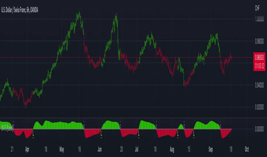
T3 Velocity Candles [Loxx]T3 Velocity Candles is a candle coloring overlay that calculates its gradient coloring using T3 velocity.
What is the T3 moving average?
Better Moving Averages Tim Tillson
November 1, 1998
Tim Tillson is a software project manager at Hewlett-Packard, with degrees in Mathematics and Computer Science. He has privately traded options and equities for 15 years.
Introduction
"Digital filtering includes the process of smoothing, predicting, differentiating, integrating, separation of signals, and removal of noise from a signal. Thus many people who do such things are actually using digital filters without realizing that they are; being unacquainted with the theory, they neither understand what they have done nor the possibilities of what they might have done."
This quote from R. W. Hamming applies to the vast majority of indicators in technical analysis . Moving averages, be they simple, weighted, or exponential, are lowpass filters; low frequency components in the signal pass through with little attenuation, while high frequencies are severely reduced.
"Oscillator" type indicators (such as MACD , Momentum, Relative Strength Index ) are another type of digital filter called a differentiator.
Tushar Chande has observed that many popular oscillators are highly correlated, which is sensible because they are trying to measure the rate of change of the underlying time series, i.e., are trying to be the first and second derivatives we all learned about in Calculus.
We use moving averages (lowpass filters) in technical analysis to remove the random noise from a time series, to discern the underlying trend or to determine prices at which we will take action. A perfect moving average would have two attributes:
It would be smooth, not sensitive to random noise in the underlying time series. Another way of saying this is that its derivative would not spuriously alternate between positive and negative values.
It would not lag behind the time series it is computed from. Lag, of course, produces late buy or sell signals that kill profits.
The only way one can compute a perfect moving average is to have knowledge of the future, and if we had that, we would buy one lottery ticket a week rather than trade!
Having said this, we can still improve on the conventional simple, weighted, or exponential moving averages. Here's how:
Two Interesting Moving Averages
We will examine two benchmark moving averages based on Linear Regression analysis.
In both cases, a Linear Regression line of length n is fitted to price data.
I call the first moving average ILRS, which stands for Integral of Linear Regression Slope. One simply integrates the slope of a linear regression line as it is successively fitted in a moving window of length n across the data, with the constant of integration being a simple moving average of the first n points. Put another way, the derivative of ILRS is the linear regression slope. Note that ILRS is not the same as a SMA ( simple moving average ) of length n, which is actually the midpoint of the linear regression line as it moves across the data.
We can measure the lag of moving averages with respect to a linear trend by computing how they behave when the input is a line with unit slope. Both SMA (n) and ILRS(n) have lag of n/2, but ILRS is much smoother than SMA .
Our second benchmark moving average is well known, called EPMA or End Point Moving Average. It is the endpoint of the linear regression line of length n as it is fitted across the data. EPMA hugs the data more closely than a simple or exponential moving average of the same length. The price we pay for this is that it is much noisier (less smooth) than ILRS, and it also has the annoying property that it overshoots the data when linear trends are present.
However, EPMA has a lag of 0 with respect to linear input! This makes sense because a linear regression line will fit linear input perfectly, and the endpoint of the LR line will be on the input line.
These two moving averages frame the tradeoffs that we are facing. On one extreme we have ILRS, which is very smooth and has considerable phase lag. EPMA has 0 phase lag, but is too noisy and overshoots. We would like to construct a better moving average which is as smooth as ILRS, but runs closer to where EPMA lies, without the overshoot.
A easy way to attempt this is to split the difference, i.e. use (ILRS(n)+EPMA(n))/2. This will give us a moving average (call it IE /2) which runs in between the two, has phase lag of n/4 but still inherits considerable noise from EPMA. IE /2 is inspirational, however. Can we build something that is comparable, but smoother? Figure 1 shows ILRS, EPMA, and IE /2.
Filter Techniques
Any thoughtful student of filter theory (or resolute experimenter) will have noticed that you can improve the smoothness of a filter by running it through itself multiple times, at the cost of increasing phase lag.
There is a complementary technique (called twicing by J.W. Tukey) which can be used to improve phase lag. If L stands for the operation of running data through a low pass filter, then twicing can be described by:
L' = L(time series) + L(time series - L(time series))
That is, we add a moving average of the difference between the input and the moving average to the moving average. This is algebraically equivalent to:
2L-L(L)
This is the Double Exponential Moving Average or DEMA , popularized by Patrick Mulloy in TASAC (January/February 1994).
In our taxonomy, DEMA has some phase lag (although it exponentially approaches 0) and is somewhat noisy, comparable to IE /2 indicator.
We will use these two techniques to construct our better moving average, after we explore the first one a little more closely.
Fixing Overshoot
An n-day EMA has smoothing constant alpha=2/(n+1) and a lag of (n-1)/2.
Thus EMA (3) has lag 1, and EMA (11) has lag 5. Figure 2 shows that, if I am willing to incur 5 days of lag, I get a smoother moving average if I run EMA (3) through itself 5 times than if I just take EMA (11) once.
This suggests that if EPMA and DEMA have 0 or low lag, why not run fast versions (eg DEMA (3)) through themselves many times to achieve a smooth result? The problem is that multiple runs though these filters increase their tendency to overshoot the data, giving an unusable result. This is because the amplitude response of DEMA and EPMA is greater than 1 at certain frequencies, giving a gain of much greater than 1 at these frequencies when run though themselves multiple times. Figure 3 shows DEMA (7) and EPMA(7) run through themselves 3 times. DEMA^3 has serious overshoot, and EPMA^3 is terrible.
The solution to the overshoot problem is to recall what we are doing with twicing:
DEMA (n) = EMA (n) + EMA (time series - EMA (n))
The second term is adding, in effect, a smooth version of the derivative to the EMA to achieve DEMA . The derivative term determines how hot the moving average's response to linear trends will be. We need to simply turn down the volume to achieve our basic building block:
EMA (n) + EMA (time series - EMA (n))*.7;
This is algebraically the same as:
EMA (n)*1.7-EMA( EMA (n))*.7;
I have chosen .7 as my volume factor, but the general formula (which I call "Generalized Dema") is:
GD (n,v) = EMA (n)*(1+v)-EMA( EMA (n))*v,
Where v ranges between 0 and 1. When v=0, GD is just an EMA , and when v=1, GD is DEMA . In between, GD is a cooler DEMA . By using a value for v less than 1 (I like .7), we cure the multiple DEMA overshoot problem, at the cost of accepting some additional phase delay. Now we can run GD through itself multiple times to define a new, smoother moving average T3 that does not overshoot the data:
T3(n) = GD ( GD ( GD (n)))
In filter theory parlance, T3 is a six-pole non-linear Kalman filter. Kalman filters are ones which use the error (in this case (time series - EMA (n)) to correct themselves. In Technical Analysis , these are called Adaptive Moving Averages; they track the time series more aggressively when it is making large moves.

T3 Striped [Loxx]Theory:
Although T3 is widely used, some of the details on how it is calculated are less known. T3 has, internally, 6 "levels" or "steps" that it uses for its calculation.
This version:
Instead of showing the final T3 value, this indicator shows those intermediate steps. This shows the "building steps" of T3 and can be used for trend assessment as well as for possible support / resistance values.
What is the T3 moving average?
Better Moving Averages Tim Tillson
November 1, 1998
Tim Tillson is a software project manager at Hewlett-Packard, with degrees in Mathematics and Computer Science. He has privately traded options and equities for 15 years.
Introduction
"Digital filtering includes the process of smoothing, predicting, differentiating, integrating, separation of signals, and removal of noise from a signal. Thus many people who do such things are actually using digital filters without realizing that they are; being unacquainted with the theory, they neither understand what they have done nor the possibilities of what they might have done."
This quote from R. W. Hamming applies to the vast majority of indicators in technical analysis . Moving averages, be they simple, weighted, or exponential, are lowpass filters; low frequency components in the signal pass through with little attenuation, while high frequencies are severely reduced.
"Oscillator" type indicators (such as MACD , Momentum, Relative Strength Index ) are another type of digital filter called a differentiator.
Tushar Chande has observed that many popular oscillators are highly correlated, which is sensible because they are trying to measure the rate of change of the underlying time series, i.e., are trying to be the first and second derivatives we all learned about in Calculus.
We use moving averages (lowpass filters) in technical analysis to remove the random noise from a time series, to discern the underlying trend or to determine prices at which we will take action. A perfect moving average would have two attributes:
It would be smooth, not sensitive to random noise in the underlying time series. Another way of saying this is that its derivative would not spuriously alternate between positive and negative values.
It would not lag behind the time series it is computed from. Lag, of course, produces late buy or sell signals that kill profits.
The only way one can compute a perfect moving average is to have knowledge of the future, and if we had that, we would buy one lottery ticket a week rather than trade!
Having said this, we can still improve on the conventional simple, weighted, or exponential moving averages. Here's how:
Two Interesting Moving Averages
We will examine two benchmark moving averages based on Linear Regression analysis.
In both cases, a Linear Regression line of length n is fitted to price data.
I call the first moving average ILRS, which stands for Integral of Linear Regression Slope. One simply integrates the slope of a linear regression line as it is successively fitted in a moving window of length n across the data, with the constant of integration being a simple moving average of the first n points. Put another way, the derivative of ILRS is the linear regression slope. Note that ILRS is not the same as a SMA ( simple moving average ) of length n, which is actually the midpoint of the linear regression line as it moves across the data.
We can measure the lag of moving averages with respect to a linear trend by computing how they behave when the input is a line with unit slope. Both SMA (n) and ILRS(n) have lag of n/2, but ILRS is much smoother than SMA .
Our second benchmark moving average is well known, called EPMA or End Point Moving Average. It is the endpoint of the linear regression line of length n as it is fitted across the data. EPMA hugs the data more closely than a simple or exponential moving average of the same length. The price we pay for this is that it is much noisier (less smooth) than ILRS, and it also has the annoying property that it overshoots the data when linear trends are present.
However, EPMA has a lag of 0 with respect to linear input! This makes sense because a linear regression line will fit linear input perfectly, and the endpoint of the LR line will be on the input line.
These two moving averages frame the tradeoffs that we are facing. On one extreme we have ILRS, which is very smooth and has considerable phase lag. EPMA has 0 phase lag, but is too noisy and overshoots. We would like to construct a better moving average which is as smooth as ILRS, but runs closer to where EPMA lies, without the overshoot.
A easy way to attempt this is to split the difference, i.e. use (ILRS(n)+EPMA(n))/2. This will give us a moving average (call it IE /2) which runs in between the two, has phase lag of n/4 but still inherits considerable noise from EPMA. IE /2 is inspirational, however. Can we build something that is comparable, but smoother? Figure 1 shows ILRS, EPMA, and IE /2.
Filter Techniques
Any thoughtful student of filter theory (or resolute experimenter) will have noticed that you can improve the smoothness of a filter by running it through itself multiple times, at the cost of increasing phase lag.
There is a complementary technique (called twicing by J.W. Tukey) which can be used to improve phase lag. If L stands for the operation of running data through a low pass filter, then twicing can be described by:
L' = L(time series) + L(time series - L(time series))
That is, we add a moving average of the difference between the input and the moving average to the moving average. This is algebraically equivalent to:
2L-L(L)
This is the Double Exponential Moving Average or DEMA , popularized by Patrick Mulloy in TASAC (January/February 1994).
In our taxonomy, DEMA has some phase lag (although it exponentially approaches 0) and is somewhat noisy, comparable to IE /2 indicator.
We will use these two techniques to construct our better moving average, after we explore the first one a little more closely.
Fixing Overshoot
An n-day EMA has smoothing constant alpha=2/(n+1) and a lag of (n-1)/2.
Thus EMA (3) has lag 1, and EMA (11) has lag 5. Figure 2 shows that, if I am willing to incur 5 days of lag, I get a smoother moving average if I run EMA (3) through itself 5 times than if I just take EMA (11) once.
This suggests that if EPMA and DEMA have 0 or low lag, why not run fast versions (eg DEMA (3)) through themselves many times to achieve a smooth result? The problem is that multiple runs though these filters increase their tendency to overshoot the data, giving an unusable result. This is because the amplitude response of DEMA and EPMA is greater than 1 at certain frequencies, giving a gain of much greater than 1 at these frequencies when run though themselves multiple times. Figure 3 shows DEMA (7) and EPMA(7) run through themselves 3 times. DEMA^3 has serious overshoot, and EPMA^3 is terrible.
The solution to the overshoot problem is to recall what we are doing with twicing:
DEMA (n) = EMA (n) + EMA (time series - EMA (n))
The second term is adding, in effect, a smooth version of the derivative to the EMA to achieve DEMA . The derivative term determines how hot the moving average's response to linear trends will be. We need to simply turn down the volume to achieve our basic building block:
EMA (n) + EMA (time series - EMA (n))*.7;
This is algebraically the same as:
EMA (n)*1.7-EMA( EMA (n))*.7;
I have chosen .7 as my volume factor, but the general formula (which I call "Generalized Dema") is:
GD (n,v) = EMA (n)*(1+v)-EMA( EMA (n))*v,
Where v ranges between 0 and 1. When v=0, GD is just an EMA , and when v=1, GD is DEMA . In between, GD is a cooler DEMA . By using a value for v less than 1 (I like .7), we cure the multiple DEMA overshoot problem, at the cost of accepting some additional phase delay. Now we can run GD through itself multiple times to define a new, smoother moving average T3 that does not overshoot the data:
T3(n) = GD ( GD ( GD (n)))
In filter theory parlance, T3 is a six-pole non-linear Kalman filter. Kalman filters are ones which use the error (in this case (time series - EMA (n)) to correct themselves. In Technical Analysis , these are called Adaptive Moving Averages; they track the time series more aggressively when it is making large moves.
Included
Alerts
Signals
Bar coloring
Loxx's Expanded Source Types
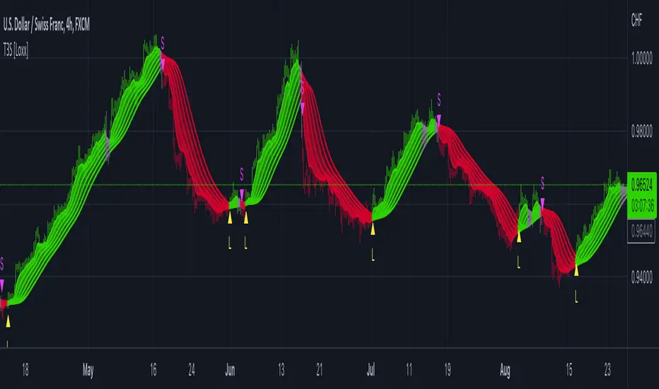
R-squared Adaptive T3 Ribbon Filled Simple [Loxx]R-squared Adaptive T3 Ribbon Filled Simple is a T3 ribbons indicator that uses a special implementation of T3 that is R-squared adaptive.
What is the T3 moving average?
Better Moving Averages Tim Tillson
November 1, 1998
Tim Tillson is a software project manager at Hewlett-Packard, with degrees in Mathematics and Computer Science. He has privately traded options and equities for 15 years.
Introduction
"Digital filtering includes the process of smoothing, predicting, differentiating, integrating, separation of signals, and removal of noise from a signal. Thus many people who do such things are actually using digital filters without realizing that they are; being unacquainted with the theory, they neither understand what they have done nor the possibilities of what they might have done."
This quote from R. W. Hamming applies to the vast majority of indicators in technical analysis . Moving averages, be they simple, weighted, or exponential, are lowpass filters; low frequency components in the signal pass through with little attenuation, while high frequencies are severely reduced.
"Oscillator" type indicators (such as MACD , Momentum, Relative Strength Index ) are another type of digital filter called a differentiator.
Tushar Chande has observed that many popular oscillators are highly correlated, which is sensible because they are trying to measure the rate of change of the underlying time series, i.e., are trying to be the first and second derivatives we all learned about in Calculus.
We use moving averages (lowpass filters) in technical analysis to remove the random noise from a time series, to discern the underlying trend or to determine prices at which we will take action. A perfect moving average would have two attributes:
It would be smooth, not sensitive to random noise in the underlying time series. Another way of saying this is that its derivative would not spuriously alternate between positive and negative values.
It would not lag behind the time series it is computed from. Lag, of course, produces late buy or sell signals that kill profits.
The only way one can compute a perfect moving average is to have knowledge of the future, and if we had that, we would buy one lottery ticket a week rather than trade!
Having said this, we can still improve on the conventional simple, weighted, or exponential moving averages. Here's how:
Two Interesting Moving Averages
We will examine two benchmark moving averages based on Linear Regression analysis.
In both cases, a Linear Regression line of length n is fitted to price data.
I call the first moving average ILRS, which stands for Integral of Linear Regression Slope. One simply integrates the slope of a linear regression line as it is successively fitted in a moving window of length n across the data, with the constant of integration being a simple moving average of the first n points. Put another way, the derivative of ILRS is the linear regression slope. Note that ILRS is not the same as a SMA ( simple moving average ) of length n, which is actually the midpoint of the linear regression line as it moves across the data.
We can measure the lag of moving averages with respect to a linear trend by computing how they behave when the input is a line with unit slope. Both SMA (n) and ILRS(n) have lag of n/2, but ILRS is much smoother than SMA .
Our second benchmark moving average is well known, called EPMA or End Point Moving Average. It is the endpoint of the linear regression line of length n as it is fitted across the data. EPMA hugs the data more closely than a simple or exponential moving average of the same length. The price we pay for this is that it is much noisier (less smooth) than ILRS, and it also has the annoying property that it overshoots the data when linear trends are present.
However, EPMA has a lag of 0 with respect to linear input! This makes sense because a linear regression line will fit linear input perfectly, and the endpoint of the LR line will be on the input line.
These two moving averages frame the tradeoffs that we are facing. On one extreme we have ILRS, which is very smooth and has considerable phase lag. EPMA has 0 phase lag, but is too noisy and overshoots. We would like to construct a better moving average which is as smooth as ILRS, but runs closer to where EPMA lies, without the overshoot.
A easy way to attempt this is to split the difference, i.e. use (ILRS(n)+EPMA(n))/2. This will give us a moving average (call it IE /2) which runs in between the two, has phase lag of n/4 but still inherits considerable noise from EPMA. IE /2 is inspirational, however. Can we build something that is comparable, but smoother? Figure 1 shows ILRS, EPMA, and IE /2.
Filter Techniques
Any thoughtful student of filter theory (or resolute experimenter) will have noticed that you can improve the smoothness of a filter by running it through itself multiple times, at the cost of increasing phase lag.
There is a complementary technique (called twicing by J.W. Tukey) which can be used to improve phase lag. If L stands for the operation of running data through a low pass filter, then twicing can be described by:
L' = L(time series) + L(time series - L(time series))
That is, we add a moving average of the difference between the input and the moving average to the moving average. This is algebraically equivalent to:
2L-L(L)
This is the Double Exponential Moving Average or DEMA , popularized by Patrick Mulloy in TASAC (January/February 1994).
In our taxonomy, DEMA has some phase lag (although it exponentially approaches 0) and is somewhat noisy, comparable to IE /2 indicator.
We will use these two techniques to construct our better moving average, after we explore the first one a little more closely.
Fixing Overshoot
An n-day EMA has smoothing constant alpha=2/(n+1) and a lag of (n-1)/2.
Thus EMA (3) has lag 1, and EMA (11) has lag 5. Figure 2 shows that, if I am willing to incur 5 days of lag, I get a smoother moving average if I run EMA (3) through itself 5 times than if I just take EMA (11) once.
This suggests that if EPMA and DEMA have 0 or low lag, why not run fast versions (eg DEMA (3)) through themselves many times to achieve a smooth result? The problem is that multiple runs though these filters increase their tendency to overshoot the data, giving an unusable result. This is because the amplitude response of DEMA and EPMA is greater than 1 at certain frequencies, giving a gain of much greater than 1 at these frequencies when run though themselves multiple times. Figure 3 shows DEMA (7) and EPMA(7) run through themselves 3 times. DEMA^3 has serious overshoot, and EPMA^3 is terrible.
The solution to the overshoot problem is to recall what we are doing with twicing:
DEMA (n) = EMA (n) + EMA (time series - EMA (n))
The second term is adding, in effect, a smooth version of the derivative to the EMA to achieve DEMA . The derivative term determines how hot the moving average's response to linear trends will be. We need to simply turn down the volume to achieve our basic building block:
EMA (n) + EMA (time series - EMA (n))*.7;
This is algebraically the same as:
EMA (n)*1.7-EMA( EMA (n))*.7;
I have chosen .7 as my volume factor, but the general formula (which I call "Generalized Dema") is:
GD (n,v) = EMA (n)*(1+v)-EMA( EMA (n))*v,
Where v ranges between 0 and 1. When v=0, GD is just an EMA , and when v=1, GD is DEMA . In between, GD is a cooler DEMA . By using a value for v less than 1 (I like .7), we cure the multiple DEMA overshoot problem, at the cost of accepting some additional phase delay. Now we can run GD through itself multiple times to define a new, smoother moving average T3 that does not overshoot the data:
T3(n) = GD ( GD ( GD (n)))
In filter theory parlance, T3 is a six-pole non-linear Kalman filter. Kalman filters are ones which use the error (in this case (time series - EMA (n)) to correct themselves. In Technical Analysis , these are called Adaptive Moving Averages; they track the time series more aggressively when it is making large moves.
What is R-squared Adaptive?
One tool available in forecasting the trendiness of the breakout is the coefficient of determination ( R-squared ), a statistical measurement.
The R-squared indicates linear strength between the security's price (the Y - axis) and time (the X - axis). The R-squared is the percentage of squared error that the linear regression can eliminate if it were used as the predictor instead of the mean value. If the R-squared were 0.99, then the linear regression would eliminate 99% of the error for prediction versus predicting closing prices using a simple moving average .
R-squared is used here to derive a T3 factor used to modify price before passing price through a six-pole non-linear Kalman filter.
Included:
Alerts
Signals
Loxx's Expanded Source Types
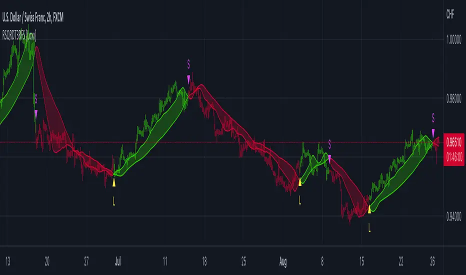
T3 Slope Variation [Loxx]T3 Slope Variation is an indicator that uses T3 moving average to calculate a slope that is then weighted to derive a signal.
The center line
The center line changes color depending on the value of the:
Slope
Signal line
Threshold
If the value is above a signal line (it is not visible on the chart) and the threshold is greater than the required, then the main trend becomes up. And reversed for the trend down.
Colors and style of the histogram
The colors and style of the histogram will be drawn if the value is at the right side, if the above described trend "agrees" with the value (above is green or below zero is red) and if the High is higher than the previous High or Low is lower than the previous low, then the according type of histogram is drawn.
What is the T3 moving average?
Better Moving Averages Tim Tillson
November 1, 1998
Tim Tillson is a software project manager at Hewlett-Packard, with degrees in Mathematics and Computer Science. He has privately traded options and equities for 15 years.
Introduction
"Digital filtering includes the process of smoothing, predicting, differentiating, integrating, separation of signals, and removal of noise from a signal. Thus many people who do such things are actually using digital filters without realizing that they are; being unacquainted with the theory, they neither understand what they have done nor the possibilities of what they might have done."
This quote from R. W. Hamming applies to the vast majority of indicators in technical analysis . Moving averages, be they simple, weighted, or exponential, are lowpass filters; low frequency components in the signal pass through with little attenuation, while high frequencies are severely reduced.
"Oscillator" type indicators (such as MACD , Momentum, Relative Strength Index ) are another type of digital filter called a differentiator.
Tushar Chande has observed that many popular oscillators are highly correlated, which is sensible because they are trying to measure the rate of change of the underlying time series, i.e., are trying to be the first and second derivatives we all learned about in Calculus.
We use moving averages (lowpass filters) in technical analysis to remove the random noise from a time series, to discern the underlying trend or to determine prices at which we will take action. A perfect moving average would have two attributes:
It would be smooth, not sensitive to random noise in the underlying time series. Another way of saying this is that its derivative would not spuriously alternate between positive and negative values.
It would not lag behind the time series it is computed from. Lag, of course, produces late buy or sell signals that kill profits.
The only way one can compute a perfect moving average is to have knowledge of the future, and if we had that, we would buy one lottery ticket a week rather than trade!
Having said this, we can still improve on the conventional simple, weighted, or exponential moving averages. Here's how:
Two Interesting Moving Averages
We will examine two benchmark moving averages based on Linear Regression analysis.
In both cases, a Linear Regression line of length n is fitted to price data.
I call the first moving average ILRS, which stands for Integral of Linear Regression Slope. One simply integrates the slope of a linear regression line as it is successively fitted in a moving window of length n across the data, with the constant of integration being a simple moving average of the first n points. Put another way, the derivative of ILRS is the linear regression slope. Note that ILRS is not the same as a SMA ( simple moving average ) of length n, which is actually the midpoint of the linear regression line as it moves across the data.
We can measure the lag of moving averages with respect to a linear trend by computing how they behave when the input is a line with unit slope. Both SMA (n) and ILRS(n) have lag of n/2, but ILRS is much smoother than SMA .
Our second benchmark moving average is well known, called EPMA or End Point Moving Average. It is the endpoint of the linear regression line of length n as it is fitted across the data. EPMA hugs the data more closely than a simple or exponential moving average of the same length. The price we pay for this is that it is much noisier (less smooth) than ILRS, and it also has the annoying property that it overshoots the data when linear trends are present.
However, EPMA has a lag of 0 with respect to linear input! This makes sense because a linear regression line will fit linear input perfectly, and the endpoint of the LR line will be on the input line.
These two moving averages frame the tradeoffs that we are facing. On one extreme we have ILRS, which is very smooth and has considerable phase lag. EPMA has 0 phase lag, but is too noisy and overshoots. We would like to construct a better moving average which is as smooth as ILRS, but runs closer to where EPMA lies, without the overshoot.
A easy way to attempt this is to split the difference, i.e. use (ILRS(n)+EPMA(n))/2. This will give us a moving average (call it IE /2) which runs in between the two, has phase lag of n/4 but still inherits considerable noise from EPMA. IE /2 is inspirational, however. Can we build something that is comparable, but smoother? Figure 1 shows ILRS, EPMA, and IE /2.
Filter Techniques
Any thoughtful student of filter theory (or resolute experimenter) will have noticed that you can improve the smoothness of a filter by running it through itself multiple times, at the cost of increasing phase lag.
There is a complementary technique (called twicing by J.W. Tukey) which can be used to improve phase lag. If L stands for the operation of running data through a low pass filter, then twicing can be described by:
L' = L(time series) + L(time series - L(time series))
That is, we add a moving average of the difference between the input and the moving average to the moving average. This is algebraically equivalent to:
2L-L(L)
This is the Double Exponential Moving Average or DEMA , popularized by Patrick Mulloy in TASAC (January/February 1994).
In our taxonomy, DEMA has some phase lag (although it exponentially approaches 0) and is somewhat noisy, comparable to IE /2 indicator.
We will use these two techniques to construct our better moving average, after we explore the first one a little more closely.
Fixing Overshoot
An n-day EMA has smoothing constant alpha=2/(n+1) and a lag of (n-1)/2.
Thus EMA (3) has lag 1, and EMA (11) has lag 5. Figure 2 shows that, if I am willing to incur 5 days of lag, I get a smoother moving average if I run EMA (3) through itself 5 times than if I just take EMA (11) once.
This suggests that if EPMA and DEMA have 0 or low lag, why not run fast versions (eg DEMA (3)) through themselves many times to achieve a smooth result? The problem is that multiple runs though these filters increase their tendency to overshoot the data, giving an unusable result. This is because the amplitude response of DEMA and EPMA is greater than 1 at certain frequencies, giving a gain of much greater than 1 at these frequencies when run though themselves multiple times. Figure 3 shows DEMA (7) and EPMA(7) run through themselves 3 times. DEMA^3 has serious overshoot, and EPMA^3 is terrible.
The solution to the overshoot problem is to recall what we are doing with twicing:
DEMA (n) = EMA (n) + EMA (time series - EMA (n))
The second term is adding, in effect, a smooth version of the derivative to the EMA to achieve DEMA . The derivative term determines how hot the moving average's response to linear trends will be. We need to simply turn down the volume to achieve our basic building block:
EMA (n) + EMA (time series - EMA (n))*.7;
This is algebraically the same as:
EMA (n)*1.7-EMA( EMA (n))*.7;
I have chosen .7 as my volume factor, but the general formula (which I call "Generalized Dema") is:
GD (n,v) = EMA (n)*(1+v)-EMA( EMA (n))*v,
Where v ranges between 0 and 1. When v=0, GD is just an EMA , and when v=1, GD is DEMA . In between, GD is a cooler DEMA . By using a value for v less than 1 (I like .7), we cure the multiple DEMA overshoot problem, at the cost of accepting some additional phase delay. Now we can run GD through itself multiple times to define a new, smoother moving average T3 that does not overshoot the data:
T3(n) = GD ( GD ( GD (n)))
In filter theory parlance, T3 is a six-pole non-linear Kalman filter. Kalman filters are ones which use the error (in this case (time series - EMA (n)) to correct themselves. In Technical Analysis , these are called Adaptive Moving Averages; they track the time series more aggressively when it is making large moves.
Included
Alets
Signals
Bar coloring
Loxx's Expanded Source Types
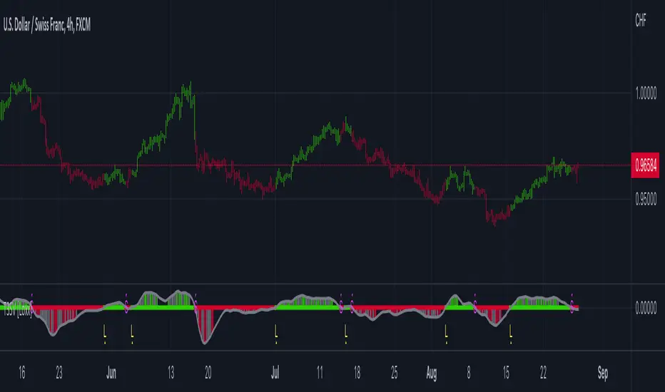
Multi T3 Slopes [Loxx]Multi T3 Slopes is an indicator that checks slopes of 5 (different period) T3 Moving Averages and adds them up to show overall trend. To us this, check for color changes from red to green where there is no red if green is larger than red and there is no red when red is larger than green. When red and green both show up, its a sign of chop.
What is the T3 moving average?
Better Moving Averages Tim Tillson
November 1, 1998
Tim Tillson is a software project manager at Hewlett-Packard, with degrees in Mathematics and Computer Science. He has privately traded options and equities for 15 years.
Introduction
"Digital filtering includes the process of smoothing, predicting, differentiating, integrating, separation of signals, and removal of noise from a signal. Thus many people who do such things are actually using digital filters without realizing that they are; being unacquainted with the theory, they neither understand what they have done nor the possibilities of what they might have done."
This quote from R. W. Hamming applies to the vast majority of indicators in technical analysis . Moving averages, be they simple, weighted, or exponential, are lowpass filters; low frequency components in the signal pass through with little attenuation, while high frequencies are severely reduced.
"Oscillator" type indicators (such as MACD , Momentum, Relative Strength Index ) are another type of digital filter called a differentiator.
Tushar Chande has observed that many popular oscillators are highly correlated, which is sensible because they are trying to measure the rate of change of the underlying time series, i.e., are trying to be the first and second derivatives we all learned about in Calculus.
We use moving averages (lowpass filters) in technical analysis to remove the random noise from a time series, to discern the underlying trend or to determine prices at which we will take action. A perfect moving average would have two attributes:
It would be smooth, not sensitive to random noise in the underlying time series. Another way of saying this is that its derivative would not spuriously alternate between positive and negative values.
It would not lag behind the time series it is computed from. Lag, of course, produces late buy or sell signals that kill profits.
The only way one can compute a perfect moving average is to have knowledge of the future, and if we had that, we would buy one lottery ticket a week rather than trade!
Having said this, we can still improve on the conventional simple, weighted, or exponential moving averages. Here's how:
Two Interesting Moving Averages
We will examine two benchmark moving averages based on Linear Regression analysis.
In both cases, a Linear Regression line of length n is fitted to price data.
I call the first moving average ILRS, which stands for Integral of Linear Regression Slope. One simply integrates the slope of a linear regression line as it is successively fitted in a moving window of length n across the data, with the constant of integration being a simple moving average of the first n points. Put another way, the derivative of ILRS is the linear regression slope. Note that ILRS is not the same as a SMA ( simple moving average ) of length n, which is actually the midpoint of the linear regression line as it moves across the data.
We can measure the lag of moving averages with respect to a linear trend by computing how they behave when the input is a line with unit slope. Both SMA (n) and ILRS(n) have lag of n/2, but ILRS is much smoother than SMA .
Our second benchmark moving average is well known, called EPMA or End Point Moving Average. It is the endpoint of the linear regression line of length n as it is fitted across the data. EPMA hugs the data more closely than a simple or exponential moving average of the same length. The price we pay for this is that it is much noisier (less smooth) than ILRS, and it also has the annoying property that it overshoots the data when linear trends are present.
However, EPMA has a lag of 0 with respect to linear input! This makes sense because a linear regression line will fit linear input perfectly, and the endpoint of the LR line will be on the input line.
These two moving averages frame the tradeoffs that we are facing. On one extreme we have ILRS, which is very smooth and has considerable phase lag. EPMA has 0 phase lag, but is too noisy and overshoots. We would like to construct a better moving average which is as smooth as ILRS, but runs closer to where EPMA lies, without the overshoot.
A easy way to attempt this is to split the difference, i.e. use (ILRS(n)+EPMA(n))/2. This will give us a moving average (call it IE /2) which runs in between the two, has phase lag of n/4 but still inherits considerable noise from EPMA. IE /2 is inspirational, however. Can we build something that is comparable, but smoother? Figure 1 shows ILRS, EPMA, and IE /2.
Filter Techniques
Any thoughtful student of filter theory (or resolute experimenter) will have noticed that you can improve the smoothness of a filter by running it through itself multiple times, at the cost of increasing phase lag.
There is a complementary technique (called twicing by J.W. Tukey) which can be used to improve phase lag. If L stands for the operation of running data through a low pass filter, then twicing can be described by:
L' = L(time series) + L(time series - L(time series))
That is, we add a moving average of the difference between the input and the moving average to the moving average. This is algebraically equivalent to:
2L-L(L)
This is the Double Exponential Moving Average or DEMA , popularized by Patrick Mulloy in TASAC (January/February 1994).
In our taxonomy, DEMA has some phase lag (although it exponentially approaches 0) and is somewhat noisy, comparable to IE /2 indicator.
We will use these two techniques to construct our better moving average, after we explore the first one a little more closely.
Fixing Overshoot
An n-day EMA has smoothing constant alpha=2/(n+1) and a lag of (n-1)/2.
Thus EMA (3) has lag 1, and EMA (11) has lag 5. Figure 2 shows that, if I am willing to incur 5 days of lag, I get a smoother moving average if I run EMA (3) through itself 5 times than if I just take EMA (11) once.
This suggests that if EPMA and DEMA have 0 or low lag, why not run fast versions (eg DEMA (3)) through themselves many times to achieve a smooth result? The problem is that multiple runs though these filters increase their tendency to overshoot the data, giving an unusable result. This is because the amplitude response of DEMA and EPMA is greater than 1 at certain frequencies, giving a gain of much greater than 1 at these frequencies when run though themselves multiple times. Figure 3 shows DEMA (7) and EPMA(7) run through themselves 3 times. DEMA^3 has serious overshoot, and EPMA^3 is terrible.
The solution to the overshoot problem is to recall what we are doing with twicing:
DEMA (n) = EMA (n) + EMA (time series - EMA (n))
The second term is adding, in effect, a smooth version of the derivative to the EMA to achieve DEMA . The derivative term determines how hot the moving average's response to linear trends will be. We need to simply turn down the volume to achieve our basic building block:
EMA (n) + EMA (time series - EMA (n))*.7;
This is algebraically the same as:
EMA (n)*1.7-EMA( EMA (n))*.7;
I have chosen .7 as my volume factor, but the general formula (which I call "Generalized Dema") is:
GD (n,v) = EMA (n)*(1+v)-EMA( EMA (n))*v,
Where v ranges between 0 and 1. When v=0, GD is just an EMA , and when v=1, GD is DEMA . In between, GD is a cooler DEMA . By using a value for v less than 1 (I like .7), we cure the multiple DEMA overshoot problem, at the cost of accepting some additional phase delay. Now we can run GD through itself multiple times to define a new, smoother moving average T3 that does not overshoot the data:
T3(n) = GD ( GD ( GD (n)))
In filter theory parlance, T3 is a six-pole non-linear Kalman filter. Kalman filters are ones which use the error (in this case (time series - EMA (n)) to correct themselves. In Technical Analysis , these are called Adaptive Moving Averages; they track the time series more aggressively when it is making large moves.
Included
Signals: long, short, continuation long, continuation short.
Alerts
Bar coloring
Loxx's expanded source types
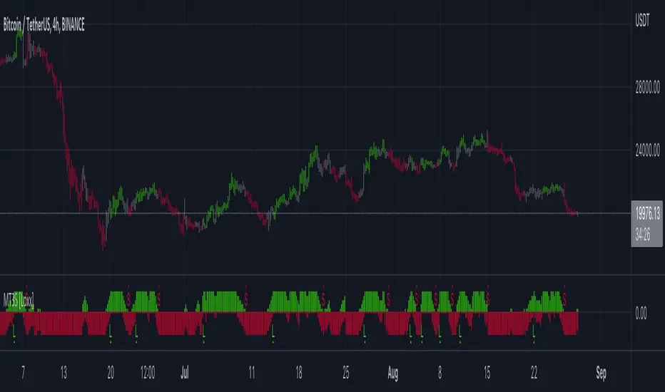
T3 Volatility Quality Index (VQI) w/ DSL & Pips Filtering [Loxx]T3 Volatility Quality Index (VQI) w/ DSL & Pips Filtering is a VQI indicator that uses T3 smoothing and discontinued signal lines to determine breakouts and breakdowns. This also allows filtering by pips.***
What is the Volatility Quality Index ( VQI )?
The idea behind the volatility quality index is to point out the difference between bad and good volatility in order to identify better trade opportunities in the market. This forex indicator works using the True Range algorithm in combination with the open, close, high and low prices.
What are DSL Discontinued Signal Line?
A lot of indicators are using signal lines in order to determine the trend (or some desired state of the indicator) easier. The idea of the signal line is easy : comparing the value to it's smoothed (slightly lagging) state, the idea of current momentum/state is made.
Discontinued signal line is inheriting that simple signal line idea and it is extending it : instead of having one signal line, more lines depending on the current value of the indicator.
"Signal" line is calculated the following way :
When a certain level is crossed into the desired direction, the EMA of that value is calculated for the desired signal line
When that level is crossed into the opposite direction, the previous "signal" line value is simply "inherited" and it becomes a kind of a level
This way it becomes a combination of signal lines and levels that are trying to combine both the good from both methods.
In simple terms, DSL uses the concept of a signal line and betters it by inheriting the previous signal line's value & makes it a level.
What is the T3 moving average?
Better Moving Averages Tim Tillson
November 1, 1998
Tim Tillson is a software project manager at Hewlett-Packard, with degrees in Mathematics and Computer Science. He has privately traded options and equities for 15 years.
Introduction
"Digital filtering includes the process of smoothing, predicting, differentiating, integrating, separation of signals, and removal of noise from a signal. Thus many people who do such things are actually using digital filters without realizing that they are; being unacquainted with the theory, they neither understand what they have done nor the possibilities of what they might have done."
This quote from R. W. Hamming applies to the vast majority of indicators in technical analysis . Moving averages, be they simple, weighted, or exponential, are lowpass filters; low frequency components in the signal pass through with little attenuation, while high frequencies are severely reduced.
"Oscillator" type indicators (such as MACD , Momentum, Relative Strength Index ) are another type of digital filter called a differentiator.
Tushar Chande has observed that many popular oscillators are highly correlated, which is sensible because they are trying to measure the rate of change of the underlying time series, i.e., are trying to be the first and second derivatives we all learned about in Calculus.
We use moving averages (lowpass filters) in technical analysis to remove the random noise from a time series, to discern the underlying trend or to determine prices at which we will take action. A perfect moving average would have two attributes:
It would be smooth, not sensitive to random noise in the underlying time series. Another way of saying this is that its derivative would not spuriously alternate between positive and negative values.
It would not lag behind the time series it is computed from. Lag, of course, produces late buy or sell signals that kill profits.
The only way one can compute a perfect moving average is to have knowledge of the future, and if we had that, we would buy one lottery ticket a week rather than trade!
Having said this, we can still improve on the conventional simple, weighted, or exponential moving averages. Here's how:
Two Interesting Moving Averages
We will examine two benchmark moving averages based on Linear Regression analysis.
In both cases, a Linear Regression line of length n is fitted to price data.
I call the first moving average ILRS, which stands for Integral of Linear Regression Slope. One simply integrates the slope of a linear regression line as it is successively fitted in a moving window of length n across the data, with the constant of integration being a simple moving average of the first n points. Put another way, the derivative of ILRS is the linear regression slope. Note that ILRS is not the same as a SMA ( simple moving average ) of length n, which is actually the midpoint of the linear regression line as it moves across the data.
We can measure the lag of moving averages with respect to a linear trend by computing how they behave when the input is a line with unit slope. Both SMA (n) and ILRS(n) have lag of n/2, but ILRS is much smoother than SMA .
Our second benchmark moving average is well known, called EPMA or End Point Moving Average. It is the endpoint of the linear regression line of length n as it is fitted across the data. EPMA hugs the data more closely than a simple or exponential moving average of the same length. The price we pay for this is that it is much noisier (less smooth) than ILRS, and it also has the annoying property that it overshoots the data when linear trends are present.
However, EPMA has a lag of 0 with respect to linear input! This makes sense because a linear regression line will fit linear input perfectly, and the endpoint of the LR line will be on the input line.
These two moving averages frame the tradeoffs that we are facing. On one extreme we have ILRS, which is very smooth and has considerable phase lag. EPMA has 0 phase lag, but is too noisy and overshoots. We would like to construct a better moving average which is as smooth as ILRS, but runs closer to where EPMA lies, without the overshoot.
A easy way to attempt this is to split the difference, i.e. use (ILRS(n)+EPMA(n))/2. This will give us a moving average (call it IE /2) which runs in between the two, has phase lag of n/4 but still inherits considerable noise from EPMA. IE /2 is inspirational, however. Can we build something that is comparable, but smoother? Figure 1 shows ILRS, EPMA, and IE /2.
Filter Techniques
Any thoughtful student of filter theory (or resolute experimenter) will have noticed that you can improve the smoothness of a filter by running it through itself multiple times, at the cost of increasing phase lag.
There is a complementary technique (called twicing by J.W. Tukey) which can be used to improve phase lag. If L stands for the operation of running data through a low pass filter, then twicing can be described by:
L' = L(time series) + L(time series - L(time series))
That is, we add a moving average of the difference between the input and the moving average to the moving average. This is algebraically equivalent to:
2L-L(L)
This is the Double Exponential Moving Average or DEMA , popularized by Patrick Mulloy in TASAC (January/February 1994).
In our taxonomy, DEMA has some phase lag (although it exponentially approaches 0) and is somewhat noisy, comparable to IE /2 indicator.
We will use these two techniques to construct our better moving average, after we explore the first one a little more closely.
Fixing Overshoot
An n-day EMA has smoothing constant alpha=2/(n+1) and a lag of (n-1)/2.
Thus EMA (3) has lag 1, and EMA (11) has lag 5. Figure 2 shows that, if I am willing to incur 5 days of lag, I get a smoother moving average if I run EMA (3) through itself 5 times than if I just take EMA (11) once.
This suggests that if EPMA and DEMA have 0 or low lag, why not run fast versions (eg DEMA (3)) through themselves many times to achieve a smooth result? The problem is that multiple runs though these filters increase their tendency to overshoot the data, giving an unusable result. This is because the amplitude response of DEMA and EPMA is greater than 1 at certain frequencies, giving a gain of much greater than 1 at these frequencies when run though themselves multiple times. Figure 3 shows DEMA (7) and EPMA(7) run through themselves 3 times. DEMA^3 has serious overshoot, and EPMA^3 is terrible.
The solution to the overshoot problem is to recall what we are doing with twicing:
DEMA (n) = EMA (n) + EMA (time series - EMA (n))
The second term is adding, in effect, a smooth version of the derivative to the EMA to achieve DEMA . The derivative term determines how hot the moving average's response to linear trends will be. We need to simply turn down the volume to achieve our basic building block:
EMA (n) + EMA (time series - EMA (n))*.7;
This is algebraically the same as:
EMA (n)*1.7-EMA( EMA (n))*.7;
I have chosen .7 as my volume factor, but the general formula (which I call "Generalized Dema") is:
GD (n,v) = EMA (n)*(1+v)-EMA( EMA (n))*v,
Where v ranges between 0 and 1. When v=0, GD is just an EMA , and when v=1, GD is DEMA . In between, GD is a cooler DEMA . By using a value for v less than 1 (I like .7), we cure the multiple DEMA overshoot problem, at the cost of accepting some additional phase delay. Now we can run GD through itself multiple times to define a new, smoother moving average T3 that does not overshoot the data:
T3(n) = GD ( GD ( GD (n)))
In filter theory parlance, T3 is a six-pole non-linear Kalman filter. Kalman filters are ones which use the error (in this case (time series - EMA (n)) to correct themselves. In Technical Analysis , these are called Adaptive Moving Averages; they track the time series more aggressively when it is making large moves.
Included
Signals
Alerts
Related indicators
Zero-line Volatility Quality Index (VQI)
Volatility Quality Index w/ Pips Filtering
Variety Moving Average Waddah Attar Explosion (WAE)
***This indicator is tuned to Forex. If you want to make it useful for other tickers, you must change the pip filtering value to match the asset. This means that for BTC, for example, you likely need to use a value of 10,000 or more for pips filter.

VHF-Adaptive T3 iTrend [Loxx]VHF-Adaptive T3 iTrend is an iTrend indicator with T3 smoothing and Vertical Horizontal Filter Adaptive period input. iTrend is used to determine where the trend starts and ends. You'll notice that the noise filter on this one is extreme. Adjust the period inputs accordingly to suit your take and your backtest requirements. This is also useful for scalping lower timeframes. Enjoy!
What is VHF Adaptive Period?
Vertical Horizontal Filter (VHF) was created by Adam White to identify trending and ranging markets. VHF measures the level of trend activity, similar to ADX DI. Vertical Horizontal Filter does not, itself, generate trading signals, but determines whether signals are taken from trend or momentum indicators. Using this trend information, one is then able to derive an average cycle length.
What is the T3 moving average?
Better Moving Averages Tim Tillson
November 1, 1998
Tim Tillson is a software project manager at Hewlett-Packard, with degrees in Mathematics and Computer Science. He has privately traded options and equities for 15 years.
Introduction
"Digital filtering includes the process of smoothing, predicting, differentiating, integrating, separation of signals, and removal of noise from a signal. Thus many people who do such things are actually using digital filters without realizing that they are; being unacquainted with the theory, they neither understand what they have done nor the possibilities of what they might have done."
This quote from R. W. Hamming applies to the vast majority of indicators in technical analysis . Moving averages, be they simple, weighted, or exponential, are lowpass filters; low frequency components in the signal pass through with little attenuation, while high frequencies are severely reduced.
"Oscillator" type indicators (such as MACD , Momentum, Relative Strength Index ) are another type of digital filter called a differentiator.
Tushar Chande has observed that many popular oscillators are highly correlated, which is sensible because they are trying to measure the rate of change of the underlying time series, i.e., are trying to be the first and second derivatives we all learned about in Calculus.
We use moving averages (lowpass filters) in technical analysis to remove the random noise from a time series, to discern the underlying trend or to determine prices at which we will take action. A perfect moving average would have two attributes:
It would be smooth, not sensitive to random noise in the underlying time series. Another way of saying this is that its derivative would not spuriously alternate between positive and negative values.
It would not lag behind the time series it is computed from. Lag, of course, produces late buy or sell signals that kill profits.
The only way one can compute a perfect moving average is to have knowledge of the future, and if we had that, we would buy one lottery ticket a week rather than trade!
Having said this, we can still improve on the conventional simple, weighted, or exponential moving averages. Here's how:
Two Interesting Moving Averages
We will examine two benchmark moving averages based on Linear Regression analysis.
In both cases, a Linear Regression line of length n is fitted to price data.
I call the first moving average ILRS, which stands for Integral of Linear Regression Slope. One simply integrates the slope of a linear regression line as it is successively fitted in a moving window of length n across the data, with the constant of integration being a simple moving average of the first n points. Put another way, the derivative of ILRS is the linear regression slope. Note that ILRS is not the same as a SMA ( simple moving average ) of length n, which is actually the midpoint of the linear regression line as it moves across the data.
We can measure the lag of moving averages with respect to a linear trend by computing how they behave when the input is a line with unit slope. Both SMA (n) and ILRS(n) have lag of n/2, but ILRS is much smoother than SMA .
Our second benchmark moving average is well known, called EPMA or End Point Moving Average. It is the endpoint of the linear regression line of length n as it is fitted across the data. EPMA hugs the data more closely than a simple or exponential moving average of the same length. The price we pay for this is that it is much noisier (less smooth) than ILRS, and it also has the annoying property that it overshoots the data when linear trends are present.
However, EPMA has a lag of 0 with respect to linear input! This makes sense because a linear regression line will fit linear input perfectly, and the endpoint of the LR line will be on the input line.
These two moving averages frame the tradeoffs that we are facing. On one extreme we have ILRS, which is very smooth and has considerable phase lag. EPMA has 0 phase lag, but is too noisy and overshoots. We would like to construct a better moving average which is as smooth as ILRS, but runs closer to where EPMA lies, without the overshoot.
A easy way to attempt this is to split the difference, i.e. use (ILRS(n)+EPMA(n))/2. This will give us a moving average (call it IE /2) which runs in between the two, has phase lag of n/4 but still inherits considerable noise from EPMA. IE /2 is inspirational, however. Can we build something that is comparable, but smoother? Figure 1 shows ILRS, EPMA, and IE /2.
Filter Techniques
Any thoughtful student of filter theory (or resolute experimenter) will have noticed that you can improve the smoothness of a filter by running it through itself multiple times, at the cost of increasing phase lag.
There is a complementary technique (called twicing by J.W. Tukey) which can be used to improve phase lag. If L stands for the operation of running data through a low pass filter, then twicing can be described by:
L' = L(time series) + L(time series - L(time series))
That is, we add a moving average of the difference between the input and the moving average to the moving average. This is algebraically equivalent to:
2L-L(L)
This is the Double Exponential Moving Average or DEMA , popularized by Patrick Mulloy in TASAC (January/February 1994).
In our taxonomy, DEMA has some phase lag (although it exponentially approaches 0) and is somewhat noisy, comparable to IE /2 indicator.
We will use these two techniques to construct our better moving average, after we explore the first one a little more closely.
Fixing Overshoot
An n-day EMA has smoothing constant alpha=2/(n+1) and a lag of (n-1)/2.
Thus EMA (3) has lag 1, and EMA (11) has lag 5. Figure 2 shows that, if I am willing to incur 5 days of lag, I get a smoother moving average if I run EMA (3) through itself 5 times than if I just take EMA (11) once.
This suggests that if EPMA and DEMA have 0 or low lag, why not run fast versions (eg DEMA (3)) through themselves many times to achieve a smooth result? The problem is that multiple runs though these filters increase their tendency to overshoot the data, giving an unusable result. This is because the amplitude response of DEMA and EPMA is greater than 1 at certain frequencies, giving a gain of much greater than 1 at these frequencies when run though themselves multiple times. Figure 3 shows DEMA (7) and EPMA(7) run through themselves 3 times. DEMA^3 has serious overshoot, and EPMA^3 is terrible.
The solution to the overshoot problem is to recall what we are doing with twicing:
DEMA (n) = EMA (n) + EMA (time series - EMA (n))
The second term is adding, in effect, a smooth version of the derivative to the EMA to achieve DEMA . The derivative term determines how hot the moving average's response to linear trends will be. We need to simply turn down the volume to achieve our basic building block:
EMA (n) + EMA (time series - EMA (n))*.7;
This is algebraically the same as:
EMA (n)*1.7-EMA( EMA (n))*.7;
I have chosen .7 as my volume factor, but the general formula (which I call "Generalized Dema") is:
GD (n,v) = EMA (n)*(1+v)-EMA( EMA (n))*v,
Where v ranges between 0 and 1. When v=0, GD is just an EMA , and when v=1, GD is DEMA . In between, GD is a cooler DEMA . By using a value for v less than 1 (I like .7), we cure the multiple DEMA overshoot problem, at the cost of accepting some additional phase delay. Now we can run GD through itself multiple times to define a new, smoother moving average T3 that does not overshoot the data:
T3(n) = GD ( GD ( GD (n)))
In filter theory parlance, T3 is a six-pole non-linear Kalman filter. Kalman filters are ones which use the error (in this case (time series - EMA (n)) to correct themselves. In Technical Analysis , these are called Adaptive Moving Averages; they track the time series more aggressively when it is making large moves.
Included
Bar coloring
Alerts
Signals
Loxx's Expanded Source Types
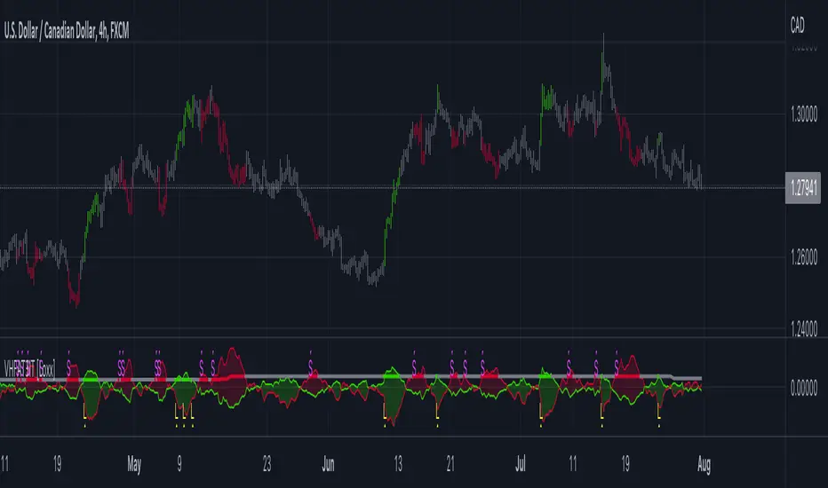
CFB-Adaptive CCI w/ T3 Smoothing [Loxx]CFB-Adaptive CCI w/ T3 Smoothing is a CCI indicator with adaptive period inputs and T3 smoothing. Jurik's Composite Fractal Behavior is used to created dynamic period input.
What is Composite Fractal Behavior ( CFB )?
All around you mechanisms adjust themselves to their environment. From simple thermostats that react to air temperature to computer chips in modern cars that respond to changes in engine temperature, r.p.m.'s, torque, and throttle position. It was only a matter of time before fast desktop computers applied the mathematics of self-adjustment to systems that trade the financial markets.
Unlike basic systems with fixed formulas, an adaptive system adjusts its own equations. For example, start with a basic channel breakout system that uses the highest closing price of the last N bars as a threshold for detecting breakouts on the up side. An adaptive and improved version of this system would adjust N according to market conditions, such as momentum, price volatility or acceleration.
Since many systems are based directly or indirectly on cycles, another useful measure of market condition is the periodic length of a price chart's dominant cycle, (DC), that cycle with the greatest influence on price action.
The utility of this new DC measure was noted by author Murray Ruggiero in the January '96 issue of Futures Magazine. In it. Mr. Ruggiero used it to adaptive adjust the value of N in a channel breakout system. He then simulated trading 15 years of D-Mark futures in order to compare its performance to a similar system that had a fixed optimal value of N. The adaptive version produced 20% more profit!
This DC index utilized the popular MESA algorithm (a formulation by John Ehlers adapted from Burg's maximum entropy algorithm, MEM). Unfortunately, the DC approach is problematic when the market has no real dominant cycle momentum, because the mathematics will produce a value whether or not one actually exists! Therefore, we developed a proprietary indicator that does not presuppose the presence of market cycles. It's called CFB (Composite Fractal Behavior) and it works well whether or not the market is cyclic.
CFB examines price action for a particular fractal pattern, categorizes them by size, and then outputs a composite fractal size index. This index is smooth, timely and accurate
Essentially, CFB reveals the length of the market's trending action time frame. Long trending activity produces a large CFB index and short choppy action produces a small index value. Investors have found many applications for CFB which involve scaling other existing technical indicators adaptively, on a bar-to-bar basis.
What is Jurik Volty used in the Juirk Filter?
One of the lesser known qualities of Juirk smoothing is that the Jurik smoothing process is adaptive. "Jurik Volty" (a sort of market volatility ) is what makes Jurik smoothing adaptive. The Jurik Volty calculation can be used as both a standalone indicator and to smooth other indicators that you wish to make adaptive.
What is the Jurik Moving Average?
Have you noticed how moving averages add some lag (delay) to your signals? ... especially when price gaps up or down in a big move, and you are waiting for your moving average to catch up? Wait no more! JMA eliminates this problem forever and gives you the best of both worlds: low lag and smooth lines.
Ideally, you would like a filtered signal to be both smooth and lag-free. Lag causes delays in your trades, and increasing lag in your indicators typically result in lower profits. In other words, late comers get what's left on the table after the feast has already begun.
What is the T3 moving average?
Better Moving Averages Tim Tillson
November 1, 1998
Tim Tillson is a software project manager at Hewlett-Packard, with degrees in Mathematics and Computer Science. He has privately traded options and equities for 15 years.
Introduction
"Digital filtering includes the process of smoothing, predicting, differentiating, integrating, separation of signals, and removal of noise from a signal. Thus many people who do such things are actually using digital filters without realizing that they are; being unacquainted with the theory, they neither understand what they have done nor the possibilities of what they might have done."
This quote from R. W. Hamming applies to the vast majority of indicators in technical analysis . Moving averages, be they simple, weighted, or exponential, are lowpass filters; low frequency components in the signal pass through with little attenuation, while high frequencies are severely reduced.
"Oscillator" type indicators (such as MACD , Momentum, Relative Strength Index ) are another type of digital filter called a differentiator.
Tushar Chande has observed that many popular oscillators are highly correlated, which is sensible because they are trying to measure the rate of change of the underlying time series, i.e., are trying to be the first and second derivatives we all learned about in Calculus.
We use moving averages (lowpass filters) in technical analysis to remove the random noise from a time series, to discern the underlying trend or to determine prices at which we will take action. A perfect moving average would have two attributes:
It would be smooth, not sensitive to random noise in the underlying time series. Another way of saying this is that its derivative would not spuriously alternate between positive and negative values.
It would not lag behind the time series it is computed from. Lag, of course, produces late buy or sell signals that kill profits.
The only way one can compute a perfect moving average is to have knowledge of the future, and if we had that, we would buy one lottery ticket a week rather than trade!
Having said this, we can still improve on the conventional simple, weighted, or exponential moving averages. Here's how:
Two Interesting Moving Averages
We will examine two benchmark moving averages based on Linear Regression analysis.
In both cases, a Linear Regression line of length n is fitted to price data.
I call the first moving average ILRS, which stands for Integral of Linear Regression Slope. One simply integrates the slope of a linear regression line as it is successively fitted in a moving window of length n across the data, with the constant of integration being a simple moving average of the first n points. Put another way, the derivative of ILRS is the linear regression slope. Note that ILRS is not the same as a SMA ( simple moving average ) of length n, which is actually the midpoint of the linear regression line as it moves across the data.
We can measure the lag of moving averages with respect to a linear trend by computing how they behave when the input is a line with unit slope. Both SMA (n) and ILRS(n) have lag of n/2, but ILRS is much smoother than SMA .
Our second benchmark moving average is well known, called EPMA or End Point Moving Average. It is the endpoint of the linear regression line of length n as it is fitted across the data. EPMA hugs the data more closely than a simple or exponential moving average of the same length. The price we pay for this is that it is much noisier (less smooth) than ILRS, and it also has the annoying property that it overshoots the data when linear trends are present.
However, EPMA has a lag of 0 with respect to linear input! This makes sense because a linear regression line will fit linear input perfectly, and the endpoint of the LR line will be on the input line.
These two moving averages frame the tradeoffs that we are facing. On one extreme we have ILRS, which is very smooth and has considerable phase lag. EPMA has 0 phase lag, but is too noisy and overshoots. We would like to construct a better moving average which is as smooth as ILRS, but runs closer to where EPMA lies, without the overshoot.
A easy way to attempt this is to split the difference, i.e. use (ILRS(n)+EPMA(n))/2. This will give us a moving average (call it IE /2) which runs in between the two, has phase lag of n/4 but still inherits considerable noise from EPMA. IE /2 is inspirational, however. Can we build something that is comparable, but smoother? Figure 1 shows ILRS, EPMA, and IE /2.
Filter Techniques
Any thoughtful student of filter theory (or resolute experimenter) will have noticed that you can improve the smoothness of a filter by running it through itself multiple times, at the cost of increasing phase lag.
There is a complementary technique (called twicing by J.W. Tukey) which can be used to improve phase lag. If L stands for the operation of running data through a low pass filter, then twicing can be described by:
L' = L(time series) + L(time series - L(time series))
That is, we add a moving average of the difference between the input and the moving average to the moving average. This is algebraically equivalent to:
2L-L(L)
This is the Double Exponential Moving Average or DEMA , popularized by Patrick Mulloy in TASAC (January/February 1994).
In our taxonomy, DEMA has some phase lag (although it exponentially approaches 0) and is somewhat noisy, comparable to IE /2 indicator.
We will use these two techniques to construct our better moving average, after we explore the first one a little more closely.
Fixing Overshoot
An n-day EMA has smoothing constant alpha=2/(n+1) and a lag of (n-1)/2.
Thus EMA (3) has lag 1, and EMA (11) has lag 5. Figure 2 shows that, if I am willing to incur 5 days of lag, I get a smoother moving average if I run EMA (3) through itself 5 times than if I just take EMA (11) once.
This suggests that if EPMA and DEMA have 0 or low lag, why not run fast versions (eg DEMA (3)) through themselves many times to achieve a smooth result? The problem is that multiple runs though these filters increase their tendency to overshoot the data, giving an unusable result. This is because the amplitude response of DEMA and EPMA is greater than 1 at certain frequencies, giving a gain of much greater than 1 at these frequencies when run though themselves multiple times. Figure 3 shows DEMA (7) and EPMA(7) run through themselves 3 times. DEMA^3 has serious overshoot, and EPMA^3 is terrible.
The solution to the overshoot problem is to recall what we are doing with twicing:
DEMA (n) = EMA (n) + EMA (time series - EMA (n))
The second term is adding, in effect, a smooth version of the derivative to the EMA to achieve DEMA . The derivative term determines how hot the moving average's response to linear trends will be. We need to simply turn down the volume to achieve our basic building block:
EMA (n) + EMA (time series - EMA (n))*.7;
This is algebraically the same as:
EMA (n)*1.7-EMA( EMA (n))*.7;
I have chosen .7 as my volume factor, but the general formula (which I call "Generalized Dema") is:
GD (n,v) = EMA (n)*(1+v)-EMA( EMA (n))*v,
Where v ranges between 0 and 1. When v=0, GD is just an EMA , and when v=1, GD is DEMA . In between, GD is a cooler DEMA . By using a value for v less than 1 (I like .7), we cure the multiple DEMA overshoot problem, at the cost of accepting some additional phase delay. Now we can run GD through itself multiple times to define a new, smoother moving average T3 that does not overshoot the data:
T3(n) = GD ( GD ( GD (n)))
In filter theory parlance, T3 is a six-pole non-linear Kalman filter. Kalman filters are ones which use the error (in this case (time series - EMA (n)) to correct themselves. In Technical Analysis , these are called Adaptive Moving Averages; they track the time series more aggressively when it is making large moves.
Included:
Bar coloring
Signals
Alerts

STD-Adaptive T3 Channel w/ Ehlers Swiss Army Knife Mod. [Loxx]STD-Adaptive T3 Channel w/ Ehlers Swiss Army Knife Mod. is an adaptive T3 indicator using standard deviation adaptivity and Ehlers Swiss Army Knife indicator to adjust the alpha value of the T3 calculation. This helps identify trends and reduce noise. In addition. I've included a Keltner Channel to show reversal/exhaustion zones.
What is the Swiss Army Knife Indicator?
John Ehlers explains the calculation here: www.mesasoftware.com
What is the T3 moving average?
Better Moving Averages Tim Tillson
November 1, 1998
Tim Tillson is a software project manager at Hewlett-Packard, with degrees in Mathematics and Computer Science. He has privately traded options and equities for 15 years.
Introduction
"Digital filtering includes the process of smoothing, predicting, differentiating, integrating, separation of signals, and removal of noise from a signal. Thus many people who do such things are actually using digital filters without realizing that they are; being unacquainted with the theory, they neither understand what they have done nor the possibilities of what they might have done."
This quote from R. W. Hamming applies to the vast majority of indicators in technical analysis . Moving averages, be they simple, weighted, or exponential, are lowpass filters; low frequency components in the signal pass through with little attenuation, while high frequencies are severely reduced.
"Oscillator" type indicators (such as MACD , Momentum, Relative Strength Index ) are another type of digital filter called a differentiator.
Tushar Chande has observed that many popular oscillators are highly correlated, which is sensible because they are trying to measure the rate of change of the underlying time series, i.e., are trying to be the first and second derivatives we all learned about in Calculus.
We use moving averages (lowpass filters) in technical analysis to remove the random noise from a time series, to discern the underlying trend or to determine prices at which we will take action. A perfect moving average would have two attributes:
It would be smooth, not sensitive to random noise in the underlying time series. Another way of saying this is that its derivative would not spuriously alternate between positive and negative values.
It would not lag behind the time series it is computed from. Lag, of course, produces late buy or sell signals that kill profits.
The only way one can compute a perfect moving average is to have knowledge of the future, and if we had that, we would buy one lottery ticket a week rather than trade!
Having said this, we can still improve on the conventional simple, weighted, or exponential moving averages. Here's how:
Two Interesting Moving Averages
We will examine two benchmark moving averages based on Linear Regression analysis.
In both cases, a Linear Regression line of length n is fitted to price data.
I call the first moving average ILRS, which stands for Integral of Linear Regression Slope. One simply integrates the slope of a linear regression line as it is successively fitted in a moving window of length n across the data, with the constant of integration being a simple moving average of the first n points. Put another way, the derivative of ILRS is the linear regression slope. Note that ILRS is not the same as a SMA ( simple moving average ) of length n, which is actually the midpoint of the linear regression line as it moves across the data.
We can measure the lag of moving averages with respect to a linear trend by computing how they behave when the input is a line with unit slope. Both SMA (n) and ILRS(n) have lag of n/2, but ILRS is much smoother than SMA .
Our second benchmark moving average is well known, called EPMA or End Point Moving Average. It is the endpoint of the linear regression line of length n as it is fitted across the data. EPMA hugs the data more closely than a simple or exponential moving average of the same length. The price we pay for this is that it is much noisier (less smooth) than ILRS, and it also has the annoying property that it overshoots the data when linear trends are present.
However, EPMA has a lag of 0 with respect to linear input! This makes sense because a linear regression line will fit linear input perfectly, and the endpoint of the LR line will be on the input line.
These two moving averages frame the tradeoffs that we are facing. On one extreme we have ILRS, which is very smooth and has considerable phase lag. EPMA has 0 phase lag, but is too noisy and overshoots. We would like to construct a better moving average which is as smooth as ILRS, but runs closer to where EPMA lies, without the overshoot.
A easy way to attempt this is to split the difference, i.e. use (ILRS(n)+EPMA(n))/2. This will give us a moving average (call it IE /2) which runs in between the two, has phase lag of n/4 but still inherits considerable noise from EPMA. IE /2 is inspirational, however. Can we build something that is comparable, but smoother? Figure 1 shows ILRS, EPMA, and IE /2.
Filter Techniques
Any thoughtful student of filter theory (or resolute experimenter) will have noticed that you can improve the smoothness of a filter by running it through itself multiple times, at the cost of increasing phase lag.
There is a complementary technique (called twicing by J.W. Tukey) which can be used to improve phase lag. If L stands for the operation of running data through a low pass filter, then twicing can be described by:
L' = L(time series) + L(time series - L(time series))
That is, we add a moving average of the difference between the input and the moving average to the moving average. This is algebraically equivalent to:
2L-L(L)
This is the Double Exponential Moving Average or DEMA , popularized by Patrick Mulloy in TASAC (January/February 1994).
In our taxonomy, DEMA has some phase lag (although it exponentially approaches 0) and is somewhat noisy, comparable to IE /2 indicator.
We will use these two techniques to construct our better moving average, after we explore the first one a little more closely.
Fixing Overshoot
An n-day EMA has smoothing constant alpha=2/(n+1) and a lag of (n-1)/2.
Thus EMA (3) has lag 1, and EMA (11) has lag 5. Figure 2 shows that, if I am willing to incur 5 days of lag, I get a smoother moving average if I run EMA (3) through itself 5 times than if I just take EMA (11) once.
This suggests that if EPMA and DEMA have 0 or low lag, why not run fast versions (eg DEMA (3)) through themselves many times to achieve a smooth result? The problem is that multiple runs though these filters increase their tendency to overshoot the data, giving an unusable result. This is because the amplitude response of DEMA and EPMA is greater than 1 at certain frequencies, giving a gain of much greater than 1 at these frequencies when run though themselves multiple times. Figure 3 shows DEMA (7) and EPMA(7) run through themselves 3 times. DEMA^3 has serious overshoot, and EPMA^3 is terrible.
The solution to the overshoot problem is to recall what we are doing with twicing:
DEMA (n) = EMA (n) + EMA (time series - EMA (n))
The second term is adding, in effect, a smooth version of the derivative to the EMA to achieve DEMA . The derivative term determines how hot the moving average's response to linear trends will be. We need to simply turn down the volume to achieve our basic building block:
EMA (n) + EMA (time series - EMA (n))*.7;
This is algebraically the same as:
EMA (n)*1.7-EMA( EMA (n))*.7;
I have chosen .7 as my volume factor, but the general formula (which I call "Generalized Dema") is:
GD (n,v) = EMA (n)*(1+v)-EMA( EMA (n))*v,
Where v ranges between 0 and 1. When v=0, GD is just an EMA , and when v=1, GD is DEMA . In between, GD is a cooler DEMA . By using a value for v less than 1 (I like .7), we cure the multiple DEMA overshoot problem, at the cost of accepting some additional phase delay. Now we can run GD through itself multiple times to define a new, smoother moving average T3 that does not overshoot the data:
T3(n) = GD ( GD ( GD (n)))
In filter theory parlance, T3 is a six-pole non-linear Kalman filter. Kalman filters are ones which use the error (in this case (time series - EMA (n)) to correct themselves. In Technical Analysis , these are called Adaptive Moving Averages; they track the time series more aggressively when it is making large moves.
Included:
Bar coloring
Signals
Alerts
Loxx's Expanded Source Types
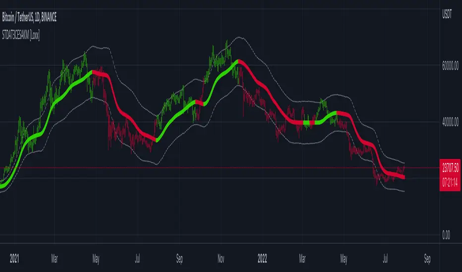
T3 Velocity [Loxx]T3 Velocity is a simple velocity indicator using T3 moving average that uses gradient colors to better identify trends.
What is the T3 moving average?
Better Moving Averages Tim Tillson
November 1, 1998
Tim Tillson is a software project manager at Hewlett-Packard, with degrees in Mathematics and Computer Science. He has privately traded options and equities for 15 years.
Introduction
"Digital filtering includes the process of smoothing, predicting, differentiating, integrating, separation of signals, and removal of noise from a signal. Thus many people who do such things are actually using digital filters without realizing that they are; being unacquainted with the theory, they neither understand what they have done nor the possibilities of what they might have done."
This quote from R. W. Hamming applies to the vast majority of indicators in technical analysis . Moving averages, be they simple, weighted, or exponential, are lowpass filters; low frequency components in the signal pass through with little attenuation, while high frequencies are severely reduced.
"Oscillator" type indicators (such as MACD , Momentum, Relative Strength Index ) are another type of digital filter called a differentiator.
Tushar Chande has observed that many popular oscillators are highly correlated, which is sensible because they are trying to measure the rate of change of the underlying time series, i.e., are trying to be the first and second derivatives we all learned about in Calculus.
We use moving averages (lowpass filters) in technical analysis to remove the random noise from a time series, to discern the underlying trend or to determine prices at which we will take action. A perfect moving average would have two attributes:
It would be smooth, not sensitive to random noise in the underlying time series. Another way of saying this is that its derivative would not spuriously alternate between positive and negative values.
It would not lag behind the time series it is computed from. Lag, of course, produces late buy or sell signals that kill profits.
The only way one can compute a perfect moving average is to have knowledge of the future, and if we had that, we would buy one lottery ticket a week rather than trade!
Having said this, we can still improve on the conventional simple, weighted, or exponential moving averages. Here's how:
Two Interesting Moving Averages
We will examine two benchmark moving averages based on Linear Regression analysis.
In both cases, a Linear Regression line of length n is fitted to price data.
I call the first moving average ILRS, which stands for Integral of Linear Regression Slope. One simply integrates the slope of a linear regression line as it is successively fitted in a moving window of length n across the data, with the constant of integration being a simple moving average of the first n points. Put another way, the derivative of ILRS is the linear regression slope. Note that ILRS is not the same as a SMA ( simple moving average ) of length n, which is actually the midpoint of the linear regression line as it moves across the data.
We can measure the lag of moving averages with respect to a linear trend by computing how they behave when the input is a line with unit slope. Both SMA (n) and ILRS(n) have lag of n/2, but ILRS is much smoother than SMA .
Our second benchmark moving average is well known, called EPMA or End Point Moving Average. It is the endpoint of the linear regression line of length n as it is fitted across the data. EPMA hugs the data more closely than a simple or exponential moving average of the same length. The price we pay for this is that it is much noisier (less smooth) than ILRS, and it also has the annoying property that it overshoots the data when linear trends are present.
However, EPMA has a lag of 0 with respect to linear input! This makes sense because a linear regression line will fit linear input perfectly, and the endpoint of the LR line will be on the input line.
These two moving averages frame the tradeoffs that we are facing. On one extreme we have ILRS, which is very smooth and has considerable phase lag. EPMA has 0 phase lag, but is too noisy and overshoots. We would like to construct a better moving average which is as smooth as ILRS, but runs closer to where EPMA lies, without the overshoot.
A easy way to attempt this is to split the difference, i.e. use (ILRS(n)+EPMA(n))/2. This will give us a moving average (call it IE /2) which runs in between the two, has phase lag of n/4 but still inherits considerable noise from EPMA. IE /2 is inspirational, however. Can we build something that is comparable, but smoother? Figure 1 shows ILRS, EPMA, and IE /2.
Filter Techniques
Any thoughtful student of filter theory (or resolute experimenter) will have noticed that you can improve the smoothness of a filter by running it through itself multiple times, at the cost of increasing phase lag.
There is a complementary technique (called twicing by J.W. Tukey) which can be used to improve phase lag. If L stands for the operation of running data through a low pass filter, then twicing can be described by:
L' = L(time series) + L(time series - L(time series))
That is, we add a moving average of the difference between the input and the moving average to the moving average. This is algebraically equivalent to:
2L-L(L)
This is the Double Exponential Moving Average or DEMA , popularized by Patrick Mulloy in TASAC (January/February 1994).
In our taxonomy, DEMA has some phase lag (although it exponentially approaches 0) and is somewhat noisy, comparable to IE /2 indicator.
We will use these two techniques to construct our better moving average, after we explore the first one a little more closely.
Fixing Overshoot
An n-day EMA has smoothing constant alpha=2/(n+1) and a lag of (n-1)/2.
Thus EMA (3) has lag 1, and EMA (11) has lag 5. Figure 2 shows that, if I am willing to incur 5 days of lag, I get a smoother moving average if I run EMA (3) through itself 5 times than if I just take EMA (11) once.
This suggests that if EPMA and DEMA have 0 or low lag, why not run fast versions (eg DEMA (3)) through themselves many times to achieve a smooth result? The problem is that multiple runs though these filters increase their tendency to overshoot the data, giving an unusable result. This is because the amplitude response of DEMA and EPMA is greater than 1 at certain frequencies, giving a gain of much greater than 1 at these frequencies when run though themselves multiple times. Figure 3 shows DEMA (7) and EPMA(7) run through themselves 3 times. DEMA^3 has serious overshoot, and EPMA^3 is terrible.
The solution to the overshoot problem is to recall what we are doing with twicing:
DEMA (n) = EMA (n) + EMA (time series - EMA (n))
The second term is adding, in effect, a smooth version of the derivative to the EMA to achieve DEMA . The derivative term determines how hot the moving average's response to linear trends will be. We need to simply turn down the volume to achieve our basic building block:
EMA (n) + EMA (time series - EMA (n))*.7;
This is algebraically the same as:
EMA (n)*1.7-EMA( EMA (n))*.7;
I have chosen .7 as my volume factor, but the general formula (which I call "Generalized Dema") is:
GD (n,v) = EMA (n)*(1+v)-EMA( EMA (n))*v,
Where v ranges between 0 and 1. When v=0, GD is just an EMA , and when v=1, GD is DEMA . In between, GD is a cooler DEMA . By using a value for v less than 1 (I like .7), we cure the multiple DEMA overshoot problem, at the cost of accepting some additional phase delay. Now we can run GD through itself multiple times to define a new, smoother moving average T3 that does not overshoot the data:
T3(n) = GD ( GD ( GD (n)))
In filter theory parlance, T3 is a six-pole non-linear Kalman filter. Kalman filters are ones which use the error (in this case (time series - EMA (n)) to correct themselves. In Technical Analysis , these are called Adaptive Moving Averages; they track the time series more aggressively when it is making large moves.
Included:
Bar coloring
Signals
Alerts
Loxx's Expanded Source Types

R-squared Adaptive T3 w/ DSL [Loxx]R-squared Adaptive T3 w/ DSL is the following T3 indicator but with Discontinued Signal Lines added to reduce noise and thereby increase signal accuracy. This adaptation makes this indicator lower TF scalp friendly.
What is R-squared Adaptive?
One tool available in forecasting the trendiness of the breakout is the coefficient of determination ( R-squared ), a statistical measurement.
The R-squared indicates linear strength between the security's price (the Y - axis) and time (the X - axis). The R-squared is the percentage of squared error that the linear regression can eliminate if it were used as the predictor instead of the mean value. If the R-squared were 0.99, then the linear regression would eliminate 99% of the error for prediction versus predicting closing prices using a simple moving average .
R-squared is used here to derive a T3 factor used to modify price before passing price through a six-pole non-linear Kalman filter.
What is the T3 moving average?
Better Moving Averages Tim Tillson
November 1, 1998
Tim Tillson is a software project manager at Hewlett-Packard, with degrees in Mathematics and Computer Science. He has privately traded options and equities for 15 years.
Introduction
"Digital filtering includes the process of smoothing, predicting, differentiating, integrating, separation of signals, and removal of noise from a signal. Thus many people who do such things are actually using digital filters without realizing that they are; being unacquainted with the theory, they neither understand what they have done nor the possibilities of what they might have done."
This quote from R. W. Hamming applies to the vast majority of indicators in technical analysis . Moving averages, be they simple, weighted, or exponential, are lowpass filters; low frequency components in the signal pass through with little attenuation, while high frequencies are severely reduced.
"Oscillator" type indicators (such as MACD , Momentum, Relative Strength Index ) are another type of digital filter called a differentiator.
Tushar Chande has observed that many popular oscillators are highly correlated, which is sensible because they are trying to measure the rate of change of the underlying time series, i.e., are trying to be the first and second derivatives we all learned about in Calculus.
We use moving averages (lowpass filters) in technical analysis to remove the random noise from a time series, to discern the underlying trend or to determine prices at which we will take action. A perfect moving average would have two attributes:
It would be smooth, not sensitive to random noise in the underlying time series. Another way of saying this is that its derivative would not spuriously alternate between positive and negative values.
It would not lag behind the time series it is computed from. Lag, of course, produces late buy or sell signals that kill profits.
The only way one can compute a perfect moving average is to have knowledge of the future, and if we had that, we would buy one lottery ticket a week rather than trade!
Having said this, we can still improve on the conventional simple, weighted, or exponential moving averages. Here's how:
Two Interesting Moving Averages
We will examine two benchmark moving averages based on Linear Regression analysis.
In both cases, a Linear Regression line of length n is fitted to price data.
I call the first moving average ILRS, which stands for Integral of Linear Regression Slope. One simply integrates the slope of a linear regression line as it is successively fitted in a moving window of length n across the data, with the constant of integration being a simple moving average of the first n points. Put another way, the derivative of ILRS is the linear regression slope. Note that ILRS is not the same as a SMA ( simple moving average ) of length n, which is actually the midpoint of the linear regression line as it moves across the data.
We can measure the lag of moving averages with respect to a linear trend by computing how they behave when the input is a line with unit slope. Both SMA (n) and ILRS(n) have lag of n/2, but ILRS is much smoother than SMA .
Our second benchmark moving average is well known, called EPMA or End Point Moving Average. It is the endpoint of the linear regression line of length n as it is fitted across the data. EPMA hugs the data more closely than a simple or exponential moving average of the same length. The price we pay for this is that it is much noisier (less smooth) than ILRS, and it also has the annoying property that it overshoots the data when linear trends are present.
However, EPMA has a lag of 0 with respect to linear input! This makes sense because a linear regression line will fit linear input perfectly, and the endpoint of the LR line will be on the input line.
These two moving averages frame the tradeoffs that we are facing. On one extreme we have ILRS, which is very smooth and has considerable phase lag. EPMA has 0 phase lag, but is too noisy and overshoots. We would like to construct a better moving average which is as smooth as ILRS, but runs closer to where EPMA lies, without the overshoot.
A easy way to attempt this is to split the difference, i.e. use (ILRS(n)+EPMA(n))/2. This will give us a moving average (call it IE /2) which runs in between the two, has phase lag of n/4 but still inherits considerable noise from EPMA. IE /2 is inspirational, however. Can we build something that is comparable, but smoother? Figure 1 shows ILRS, EPMA, and IE /2.
Filter Techniques
Any thoughtful student of filter theory (or resolute experimenter) will have noticed that you can improve the smoothness of a filter by running it through itself multiple times, at the cost of increasing phase lag.
There is a complementary technique (called twicing by J.W. Tukey) which can be used to improve phase lag. If L stands for the operation of running data through a low pass filter, then twicing can be described by:
L' = L(time series) + L(time series - L(time series))
That is, we add a moving average of the difference between the input and the moving average to the moving average. This is algebraically equivalent to:
2L-L(L)
This is the Double Exponential Moving Average or DEMA , popularized by Patrick Mulloy in TASAC (January/February 1994).
In our taxonomy, DEMA has some phase lag (although it exponentially approaches 0) and is somewhat noisy, comparable to IE /2 indicator.
We will use these two techniques to construct our better moving average, after we explore the first one a little more closely.
Fixing Overshoot
An n-day EMA has smoothing constant alpha=2/(n+1) and a lag of (n-1)/2.
Thus EMA (3) has lag 1, and EMA (11) has lag 5. Figure 2 shows that, if I am willing to incur 5 days of lag, I get a smoother moving average if I run EMA (3) through itself 5 times than if I just take EMA (11) once.
This suggests that if EPMA and DEMA have 0 or low lag, why not run fast versions (eg DEMA (3)) through themselves many times to achieve a smooth result? The problem is that multiple runs though these filters increase their tendency to overshoot the data, giving an unusable result. This is because the amplitude response of DEMA and EPMA is greater than 1 at certain frequencies, giving a gain of much greater than 1 at these frequencies when run though themselves multiple times. Figure 3 shows DEMA (7) and EPMA(7) run through themselves 3 times. DEMA^3 has serious overshoot, and EPMA^3 is terrible.
The solution to the overshoot problem is to recall what we are doing with twicing:
DEMA (n) = EMA (n) + EMA (time series - EMA (n))
The second term is adding, in effect, a smooth version of the derivative to the EMA to achieve DEMA . The derivative term determines how hot the moving average's response to linear trends will be. We need to simply turn down the volume to achieve our basic building block:
EMA (n) + EMA (time series - EMA (n))*.7;
This is algebraically the same as:
EMA (n)*1.7-EMA( EMA (n))*.7;
I have chosen .7 as my volume factor, but the general formula (which I call "Generalized Dema") is:
GD (n,v) = EMA (n)*(1+v)-EMA( EMA (n))*v,
Where v ranges between 0 and 1. When v=0, GD is just an EMA , and when v=1, GD is DEMA . In between, GD is a cooler DEMA . By using a value for v less than 1 (I like .7), we cure the multiple DEMA overshoot problem, at the cost of accepting some additional phase delay. Now we can run GD through itself multiple times to define a new, smoother moving average T3 that does not overshoot the data:
T3(n) = GD ( GD ( GD (n)))
In filter theory parlance, T3 is a six-pole non-linear Kalman filter. Kalman filters are ones which use the error (in this case (time series - EMA (n)) to correct themselves. In Technical Analysis , these are called Adaptive Moving Averages; they track the time series more aggressively when it is making large moves.
Included:
Bar coloring
Signals
Alerts
EMA and FEMA Signla/DSL smoothing
Loxx's Expanded Source Types