Trend Channels (MTF) | Flux Charts💎 GENERAL OVERVIEW
Introducing our new Trend Channels (MTF) indicator! Latest trends play an important role for traders and sometimes it can be hard to spot trends in other timeframes. This indicator can plot latest trend channels across different timeframes, so you can spot trends and their channels easier. More info about the process in the "How Does It Work" section.
Features of the new Trend Channels (MTF) indicator :
Plot Trend Channels Across Up To 3 Different Timeframes
Broad Customizability Of Trend Detection
Variety Of Trend Invalidation Options
High Visual Customizability
🚩UNIQUENESS
While the detection of trend channels is a common concept among traders, trend channels across different timeframes can be as crucial as the ones in the current timeframe. This indicator can find them from up to 3 different timeframes. While the general settings will perform well enough most of the time, the indicator also provides fine-tuning options for trend detection and trend invalidation for more experienced traders.
📌 HOW DOES IT WORK ?
Trend channels occur when the price of an asset starts making a strong movement in a bullish or a bearish direction. This indicator detects trend channels using the Simple Moving Average (SMA). When the slope of the SMA line exceeds the user-defined size, a trend channel will occur.
To understand how individual settings work, you can check the "⚙️SETTINGS" section.
⚙️SETTINGS
1. General Configuration
SMA Length -> Determines the length used in the SMA function. Higher values mean that an average of a longer timespan will be taken into account when spotting trends.
Slope Length -> Used while finding the slope of the trend channel. Check this example for slope length :
ATR Size -> This setting is taken into calculation while checking if a trend channel is worth plotting. The higher this setting is, the higher the slope of the trend channel must be to get rendered. You can take a look at the chart provided above for a visual explanation.
Channel Expander -> When a trend channel occurs, the top and the bottom of the channel are initally determined by the latest highest highs / lowest lows. This setting expands the channel vertically by X times Average True Range (ATR). Check this example :
Trend Invalidation -> The trend channel gets invalidated when the bar closes / wicks above the top of the channel, or below the bottom of the channel. With this setting, you can switch the behaviour between bar close / bar wick.
Avoid False Invalidation -> This setting makes it harder for trend channels to get invalidated to prevent false invalidations.
Retries : The trend channel will have 5 chances for invalidation. First 4 invalidations will not invalidate the channel. The trend channel will only invalidate once the 5th invalidation occur.
Volume : The bar that invalidates the trend channel must have a volume higher than 1.5x the average bar volume of the current chart. Otherwise the trend channel will not be invalidated.
None : The trend channel will invalidate at the first invalidation.
Search in scripts for "TAKE"

Volatility System by W. WilderVolatility System (Volatility Stops) Similarity
Most traders adjust their stops over time in the direction of the trend in order to lock in profits. Apart from moving averages, one of the most popular techniques is trailing stops using a multiple of Average True Range. There are several variations:
The original Volatility System(Volatility Stops), introduced by Welles Wilder in his 1978 book: New Concepts in Technical Trading Systems
Chandelier exits introduced by Alexander Elder in Come Into My Trading Room (2002) trail the stops from Highs or Lows rather than Closing Price
Average True Range Trailing Stops are similar to the above, but include a ratchet mechanism to prevent stops moving down during an up-trend or rising during a down-trend, as ATR increases
WillTrend intoduced by Larry Williams in 1988
Comparison of systems
All the systems under consideration have one common ingredient - ATR. ATR was developed by Welles Wilder and described in his book in 1978, also in this book the Volatility System was described, which in the future became known as Volatility Stops.
In fact, Wilder is the father of such systems due to the presence of ATR in the calculation of this type of indicator.
The main difference of Volatility System
Followers such as Larry Williams and Alexander Elder made minor changes to the value based on the ATR, mainly focusing on changing the base to which this value is added or subtracted.
Larry Williams uses the square root of 5 as a multiplier and calculates the ATR with a period of 66, and Alexander Elder uses a multiplier of 2.5-3.5 applying it to the ATR with a period of 22. Both authors changed the original value for ATR and multiplier calculations. Alexander Elder is closest to the original Welles Wilder calculation, which used a multiplier of 2.8.-3.1 applying it to an ATR with a period of 7.
As a reference, Elder took the Highest High(22) from which he subtracts ATR*Multiplier in an uptrend or the Lowest Low(22) to which he adds ATR*Multiplier to obtain the turning point (SAR).
Larry Williams uses the average price of extremes (Highest High(10) + Lowest Low(10)) / 2 as a reference base to which he adds or subtracts the ATR*Multilpyer values.
Both systems differ from the original, because Wilder used Significan Close(SIC) in his calculations. SIC is the maximum closing price during an uptrend and the minimum closing price during a downtrend, which
does not go beyond the current trade, as in other systems. To calculate the base when a trend changes, bars that are outside the current trend will be used when calculating WillTrend and Chandelier Exit, in contrast to the Volatility System, which takes SIC values only within the current trade. This is the main difference from subsequent developments of similar systems.
Improvements made
The original Volatility System is present as an indicator on TradingView, but it is an improved version with the addition of a ratchet and works differently from the original Weilder system.
List of improvements:
Added the ability to remove the ratchet. You need to turn off the "Trail one way" checkbox in the setting menu. When this function is turned off, the system will operate in the author-inventor mode. On some instruments, the original system works much better than the improved ratchet system, which cannot be turned off.
Added the ability to use Highest High and Lowest Low as a base instead of the closing price.
Volatility Stops Formula Description
Welles Wilder's system uses Closing Price and incorporates a stop-and-reverse feature (as with his Parabolic SAR).
Determine the initial trend direction
Calculate the Significant Close ("SIC"): the highest close reached in an up-trend or the lowest close in a down-trend
Calculate Average True Range ("ATR") for the selected period (7 days in this example)
Multiply ATR by the Multiple (3.0 in this example, best values author describes as 2.8-3.1)
The first stop is calculated in day 7 and plotted for day 8
If an up-trend, the first stop is SIC - 3 * ATR, otherwise SIC + 3 * ATR for a down-trend
Repeat each day until price closes below the stop (or above in a down-trend)
Set SIC equal to the latest Close, reverse the trend and continue.
Chandelier Exit Description
Chandelier Exits subtract a multiple of Average True Range ("ATR") from the highest high for the selected period. Using the default settings as an example:
Highest High in last 22 days - 3 * ATR for 22 days
In a down-trend the formula is reversed:
Lowest Low in last 22 days + 3 * ATR for 22 days
The time period must be long enough to capture the highest point of the recent up-trend: too short and the stops move downward; too long and the high may be taken from a previous down-trend.
It is not essential to use the same period for up and down trends; down-trends are notoriously faster than up-trends and may benefit from a shorter time period.
The multiple of 3 may be varied, but most traders settle between 2.5 and 3.5.
WillTrend Description
Larry Williams is prefer to used the Square Root from 5 as a multiplayer for ATR. SQRT(5) = 2.236
WillTrend subtract a multiple of Average True Range ("ATR") from the Middle Price (Highest High for the selected period + Lowest Low for the selected period / 2).
(Highest High in last 10 days + Lowest Low in last 10 days) / 2 - 2.236 * ATR for 66 days
In a down-trend the formula is reversed:
(Highest High in last 10 days + Lowest Low in last 10 days) / 2 + 2.236 * ATR for 66 days

Blockunity Excess Index (BEI)Identify excess zones resulting in market reversals by visualizing price deviations from an average.
The Excess Index (BEI) is designed to identify excess zones resulting in reversals, based on price deviations from a moving average. This moving average is fully customizable (type, period to be taken into account, etc.). This indicator also multiplies the moving average with a configurable coefficient, to give dynamic support and resistance levels. Finally, the BEI also provides reversal signals to alert you to any risk of trend change, on any asset.
The Idea
The goal is to provide the community with a visual and customizable tool for analyzing large price deviations from an average.
How to Use
Very simple to use, this indicator plots colored zones according to the price's deviation from the moving average. Moving average extensions also provide dynamic support and resistance. Finally, signals alert you to potential reversal points.
Elements
The Moving Average
The Moving Average, which defaults to a gray line over 200 periods, serves as a stable reference point. It is accompanied by an Index, whose color varies from yellow to orange to red, offering an overview of market conditions.
Extensions
These dynamic lines can be used to determine effective supports and resistances.
Signals
Green and red triangles serve as clear indicators for buy and sell signals.
Settings
Mainly, the type of moving average is configurable. The default is an SMA.
A Simple Moving Average (SMA) calculates the average of a selected range of prices by the number of periods in that range.
But you can also, for example, switch the mode to EMA.
The Exponential Moving Average (EMA) is a moving average that places a greater weight and significance on the most recent data points:
You also have WMA.
A Weighted Moving Average (WMA) gives more weight on recent data and less on past data:
And finally, the possibility of having a PCMA.
PCMA takes into account the highest and lowest points in the lookback period and divides this by two to obtain an average:
You can change other parameters such as lookback periods, as well as the coefficient used to define extension lines.
You can refer to the tooltips directly in the indicator parameters.
For those who prefer a minimalist display, you can activate a "Bar Color" in the settings (You must also uncheck "Borders" and "Wick" in your Chart Settings), and deactivate all other elements as you wish:
Finally, you can customize all the different colors, as well as the parameters of the table that indicates the Index value and the asset trend.
How it Works
The Index is calculated using the following method:
abs_distance = math.abs(close - base_ma)
bei = (abs_distance - ta.lowest(abs_distance, lookback_norm)) / (ta.highest(abs_distance, lookback_norm) - ta.lowest(abs_distance, lookback_norm)) * 100
Signals are triggered according to the following conditions:
A Long (buy) signal is triggered when the Index falls below 100, when the closing price is lower than 5 periods ago, and when the price is under the moving average.
A Short (sell) signal is triggered when the Index falls below 100, when the closing price is greater than 5 periods ago, and when the price is above the moving average.

Goldmine Wealth Builder - DKK/SKKGoldmine Wealth Builder
Version 1.0
Introduction to Long-Term Investment Strategies: DKK, SKK1 and SKK2
In the dynamic realm of long-term investing, the DKK, SKK1, and SKK2 strategies stand as valuable pillars. These strategies, meticulously designed to assist investors in building robust portfolios, combine the power of Super Trend, RSI (Relative Strength Index), Exponential Moving Averages (EMAs), and their crossovers. By providing clear alerts and buy signals on a daily time frame, they equip users with the tools needed to make well-informed investment decisions and navigate the complexities of the financial markets. These strategies offer a versatile and structured approach to both conservative and aggressive investment, catering to the diverse preferences and objectives of investors.
Each part of this strategy provides a unique perspective and approach to the accumulation of assets, making it a versatile and comprehensive method for investors seeking to optimize their portfolio performance. By diligently applying this multi-faceted approach, investors can make informed decisions and effectively capitalize on potential market opportunities.
DKK Strategy for ETFs and Funds:
The DKK system is a strategy designed for accumulating ETFs and Funds as long-term investments in your portfolio. It simplifies the process of identifying trend reversals and opportune moments to invest in listed ETFs and Funds, particularly during bull markets. Here's a detailed explanation of the DKK system:
Objective: The primary aim of the DKK system is to build a long-term investment portfolio by focusing on ETFs and Funds. It facilitates the identification of stocks that are in the process of reversing their trends, allowing investors to benefit from upward price movements in these financial instruments.
Stock Selection Criteria: The DKK system employs specific criteria for selecting ETFs and Funds:
• 200EMA (Exponential Moving Average): The system monitors whether the prices of ETFs and Funds are consistently below the 200-day Exponential Moving Average. This is considered an indicator of weakness, especially on a daily time frame.
• RSI (Relative Strength Index): The system looks for an RSI value of less than 40. An RSI below 40 is often seen as an indication of a weak or oversold condition in a financial instrument.
Alert Signal: Once the DKK system identifies ETFs and Funds meeting these criteria, it provides an alert signal:
• Red Upside Triangle Sign: This signal is automatically generated on the daily chart of ETFs and Funds. It serves as a clear indicator to investors that it's an opportune time to accumulate these financial instruments for long-term investment.
It's important to note that the DKK system is specifically designed for ETFs and Funds, so it should be applied to these types of investments. Additionally, it's recommended to track index ETFs and specific types of funds, such as REITs (Real Estate Investment Trusts) and INVITs (Infrastructure Investment Trusts), in line with the DKK system's approach. This strategy simplifies the process of identifying investment opportunities within this asset class, particularly during periods of market weakness.
SKK1 Strategy for Conservative Stock Investment:
The SKK 1 system is a stock investment strategy tailored for conservative investors seeking long-term portfolio growth with a focus on stability and prudent decision-making. This strategy is meticulously designed to identify pivotal market trends and stock price movements, allowing investors to make informed choices and capitalize on upward market trends while minimizing risk. Here's a comprehensive overview of the SKK 1 system, emphasizing its suitability for conservative investors:
Objective: The primary objective of the SKK 1 system is to accumulate stocks as long-term investments in your portfolio while prioritizing capital preservation. It offers a disciplined approach to pinpointing potential entry points for stocks, particularly during market corrections and trend reversals, thereby enabling you to actively participate in bullish market phases while adopting a conservative risk management stance.
Stock Selection Criteria: The SKK 1 system employs a stringent set of criteria to select stocks for investment:
• Correction Mode: It identifies stocks that have undergone a correction, signifying a decline in stock prices from their recent highs. This conservative approach emphasizes the importance of seeking stocks with a history of stability.
• 200EMA (Exponential Moving Average): The system diligently analyses daily stock price movements, specifically looking for stocks that have fallen to or below the 200-day Exponential Moving Average. This indicator suggests potential overselling and aligns with a conservative strategy of buying low.
Trend Reversal Confirmation: The SKK 1 system doesn't merely pinpoint stocks in correction mode; it takes an extra step to confirm a trend reversal. It employs the following indicators:
• Short-term Downtrends Reversal: This aspect focuses on identifying the reversal of short-term downtrends in stock prices, observed through the transition of the super trend indicator from the red zone to the green zone. This cautious approach ensures that the trend is genuinely shifting.
• Super Trend Zones: These zones are crucial for assessing whether a stock is in a bullish or bearish trend. The system consistently monitors these zones to confirm a potential trend reversal.
Alert & Buy Signals: When the SKK 1 system identifies stocks that have reached a potential bottom and are on the verge of a trend reversal, it issues vital alert signals, aiding conservative investors in prudent decision-making:
• Orange Upside Triangle Sign: This signal serves as a cautious heads-up, indicating that a stock may be poised for a trend reversal. It advises investors to prepare funds for potential investment without taking undue risks.
• Green Upside Triangle Sign: This is the confirmation of a trend reversal, signifying a robust buy signal. Conservative investors can confidently enter the market at this point, accumulating stocks for a long-term investment, secure in the knowledge that the trend is in their favor.
In summary, the SKK 1 system is a systematic and conservative approach to stock investing. It excels in identifying stocks experiencing corrections and ensures that investors act when there's a strong indication of a trend reversal, all while prioritizing capital preservation and risk management. This strategy empowers conservative investors to navigate the intricacies of the stock market with confidence, providing a calculated and stable path toward long-term portfolio growth.
Note: The SKK1 strategy, known for its conservative approach to stock investment, also provides an option to extend its methodology to ETFs and Funds for those investors who wish to accumulate assets more aggressively. By enabling this feature in the settings, you can harness the SKK1 strategy's careful criteria and signal indicators to accumulate aggressive investments in ETFs and Funds.
This flexible approach acknowledges that even within a conservative strategy, there may be opportunities for more assertive investments in assets like ETFs and Funds. By making use of this option, you can strike a balance between a conservative stance in your stock portfolio while exploring an aggressive approach in other asset classes. It offers the versatility to cater to a variety of investment preferences, ensuring that you can adapt your strategy to suit your financial goals and risk tolerance.
SKK 2 Strategy for Aggressive Stock Investment:
The SKK 2 strategy is designed for those who are determined not to miss significant opportunities within a continuous uptrend and seek a way to enter a trend that doesn't present entry signals through the SKK 1 strategy. While it offers a more aggressive entry approach, it is ideal for individuals willing to take calculated risks to potentially reap substantial long-term rewards. This strategy is particularly suitable for accumulating stocks for aggressive long-term investment. Here's a detailed description of the SKK 2 strategy:
Objective: The primary aim of the SKK 2 strategy is to provide an avenue for investors to identify short-term trend reversals and seize the opportunity to enter stocks during an uptrend, thereby capitalizing on a sustained bull run. It acknowledges that there may not always be clear entry signals through the SKK 1 strategy and offers a more aggressive alternative.
Stock Selection Criteria: The SKK 2 strategy utilizes a specific set of criteria for stock selection:
1. 50EMA (Exponential Moving Average): It targets stocks that are trading below the 50-day Exponential Moving Average. This signals a short-term reversal from the top and indicates that the stock is in a downtrend.
2. RSI (Relative Strength Index): The strategy considers stocks with an RSI of less than 40, which is an indicator of weakness in the stock.
Alert Signals: The SKK 2 strategy provides distinct alert signals that facilitate entry during an aggressive reversal:
• Red Downside Triangle Sign: This signal is triggered when the stock is below the 50EMA and has an RSI of less than 40. It serves as a clear warning of a short-term reversal from the top and a downtrend, displayed on the daily chart.
• Purple Upside Triangle Sign: This sign is generated when a reversal occurs through a bullish candle, and the RSI is greater than 40. It signifies the stock has bottomed out from a short-term downtrend and is now reversing. This purple upside triangle serves as an entry signal on the chart, presenting an attractive opportunity to accumulate stocks during a strong bullish phase, offering a chance to seize a potentially favorable long-term investment.
In essence, the SKK 2 strategy caters to aggressive investors who are willing to take calculated risks to enter stocks during a continuous uptrend. It focuses on identifying short-term reversals and provides well-defined signals for entry. While this strategy is more aggressive in nature, it has the potential to yield substantial rewards for those who are comfortable with a higher level of risk and are looking for opportunities to build a strong long-term portfolio.
Introduction to Strategy Signal Information Chart
This chart provides essential information on strategy signals for DKK, SKK1, and SKK2. By quickly identifying "Buy" and "Alert" signals for each strategy, investors can efficiently gauge market conditions and make informed decisions to optimize their investment portfolios.
In Conclusion
These investment strategies, whether conservative like DKK and SKK1 or more aggressive like SKK2, offer a range of options for investors to navigate the complex world of long-term investments. The combination of Super Trend, RSI, and EMAs with their crossovers provides clear signals on a daily time frame, empowering users to make well-informed decisions and potentially capitalize on market opportunities. Whether you're looking for stability or are ready to embrace more risk, these strategies have something to offer for building and growing your investment portfolio.

Risk Reward Optimiser [ChartPrime]█ CONCEPTS
In modern day strategy optimization there are few options when it comes to optimizing a risk reward ratio. Users frequently need to experiment and go through countless permutations in order to tweak, adjust and find optimal in their data.
Therefore we have created the Risk Reward Optimizer.
The Risk Reward Optimizer is a technical tool designed to provide traders with comprehensive insights into their trading strategies.
It offers a range of features and functionalities aimed at enhancing traders' decision-making process.
With a focus on comprehensive data, it is there to help traders quickly and efficiently locate Risk Reward optimums for inbuilt of custom strategies.
█ Internal and external Signals:
The script can optimize risk to reward ratio for any type of signals
You can utilize the following :
🔸Internal signals ➞ We have included a number of common indicators into the optimizer such as:
▫️ Aroon
▫️ AO (Awesome Oscillator)
▫️ RSI (Relative Strength Index)
▫️ MACD (Moving Average Convergence Divergence)
▫️ SuperTrend
▫️ Stochastic RSI
▫️ Stochastic
▫️ Moving averages
All these indicators have 3 conditions to generate signals :
Crossover
High Than
Less Than
🔸External signal
▫️ by incorporating your own indicators into the analysis. This flexibility enables you to tailor your strategy to your preferences.
◽️ How to link your signal with the optimizer:
In order to be able to analysis your signal we need to read it and to do so we would need to PLOT your signal with a defined value
plot( YOUR LONG Condition ? 100 : 0 , display = display.data_window)
█ Customizable Risk to Reward Ratios:
This tool allows you to test seven different customizable risk to reward ratios , helping you determine the most suitable risk-reward balance for your trading strategy. This data-driven approach takes the guesswork out of setting stop-loss and take-profit levels.
█ Comprehensive Data Analysis:
The tool provides a table displaying key metrics, including:
Total trades
Wins
Losses
Profit factor
Win rate
Profit and loss (PNL)
This data is essential for refining your trading strategy.
🔸 It includes a tooltip for each risk to reward ratio which gives data for the:
Most Profitable Trade USD value
Most Profitable Trade % value
Most Profitable Trade Bar Index
Most Profitable Trade Time (When it occurred)
Position and size is adjustable
█ Visual insights with histograms:
Visualize your trading performance with histograms displaying each risk to reward ratio trade space, showing total trades, wins, losses, and the ratio of profitable trades.
This visual representation helps you understand the strengths and weaknesses of your strategy.
It offers tooltips for each RR ratio with the average win and loss percentages for further analysis.
█ Dynamic Highlighting:
A drop-down menu allows you to highlight the maximum values of critical metrics such as:
Profit factor
Win rate
PNL
for quick identification of successful setups.
█ Stop Loss Flexibility:
You can adjust stop-loss levels using three different calculation methods:
ATR
Pivot
VWAP
This allows you to align risk-reward ratios with your preferred risk tolerance.
█ Chart Integration:
Visualize your trades directly on your price chart, with each trade displayed in a distinct color for easy tracking.
When your take-profit (TP) level is reached , the tool labels the corresponding risk-reward ratio for that specific TP, simplifying trade management.
█ Detailed Tooltips:
Tooltips provide deeper insights into your trading performance. They include information about the most profitable trade, such as the time it occurred, the bar index, and the percentage gain. Histogram tooltips also offer average win and loss percentages for further analysis.
█ Settings:
█ Code:
In summary, the Risk Reward Optimizer is a data-driven tool that offers traders the ability to optimize their risk-reward ratios, refine their strategies, and gain a deeper understanding of their trading performance. Whether you're a day trader, swing trader, or investor, this tool can help you make informed decisions and improve your trading outcomes.

IU Break of any session StrategyHow this script works:
1. This script is an intraday trading strategy script which buy and sell on the bases of user-defined intraday session range breakout and gives alert(if the alert is set) message too when the new position is open.
2. It calculate the session as per the user inputs or user defined custom session.
3. The script stores the highest and lowest value of the whole session.
4. It take a long position on the first break and close above the highest value.
5. It take a short position on the break and close below the lowest value.
6. The script takes one position in one day.
7. The stop loss for this script is the previous low(if long) or high(if short).
8. Take profit is 1:2 and it's adjustable.
9. This script work on every kind of market.
How The Useful For The User :
1. User can backtest any session range breakout he wants to trade.
2. User can get alert when the new position is open.
3. User can change the Risk to Reward in order to find the best Risk to Reward.
4. User can see the highest and lowest value of the session with respect to analyzing his trading objective.
5. This strategy script highlights which session range breakout performs best and which performs worst.

IU Probability CalculatorHow This Script Works:
1. This script calculate the probability of price reaching a user-defined price level within one candle with the help Normal Distribution Probability Table.
2. Normal Distribution Probability Table is use for calculating probability of events, it's very powerful for calculation of probability and this script is fully based on that table.
3. It takes the Average True Range value or Standard Deviation value of past user-defined length bar.
4. After that it take this formula z = ( price_level - close ) / (ATR or Standard Deviation) and return the value for z, for the bearish side it take z = (close - price level) / (ATR or Standard Deviation ) formula.
5. Once we have the z it look into Normal Distribution Probability Table and match the value.
6. Now the value of z is multiple buy 100 in order to make it look in percentage term.
7. After that this script subtract the final value with 100 because probability always comes under 100%
8. finally we plot the probability at the bottom of the chart the red line indicates "The probability of price not reaching that price level", While the green line indicates "Probability of price Reaching that level " .
9. This script will work fine for both of the directions
How This Is Useful For The User:
1. With this script user can know the probability of price reaching the certain level within one candle for both Directions .
2. This is useful while creating options hedging strategies
3. This can be helpful for deciding stop loss level.
4. It's useful for scalpers for managing their traders and it can be use by binary option traders.

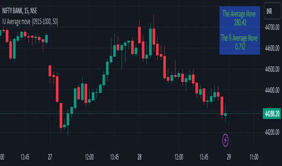
IU Average move How The Script Works :
1. This script calculate the average movement of the price in a user defined custom session and plot the data in a table from on top left corner of the chart.
2. The script takes highest and lowest value of that custom session and store their difference into an array.
3. Then the script average the array thus gets the average price.
4. Addition to that the script converter the price pip change into percentage in order to calculate the value in percentage form.
5. This script is pure price action based the script only take price value and doesn't take any indicator for calculation.
6. The script works on every type of market.
7. If the session is invalid it returns nothing
8. The background color, text color and transparency is changeable.
How User Can Benefit From This Script:
1. User can understand the volatility of any session that he/she wish to trade.
2. It can be helpful for understanding the average price moment of any tradeble asset.
3. It will give the average price movement both in percentage and points bases.
4. By understanding the volatility user can adjust his stop loss or take profit with respect his risk management.
VWAP with CharacterizationThis indicator is a visual representation of the VWAP (Volume Weighted Average Price), it calculates the weighted average price based on trading volume. Essentially, it provides a measure of the average price at which an asset has traded during a given period, but with a particular focus on trading volume. In our case, the indicator calculates the VWAP for the current trading symbol, using a predefined simple moving average (SMA) with a period of 14. This volume-weighted moving average offers a clearer view of the behavior of the VWAP and, of consequence of market dynamics.
One of the distinctive features of this indicator is its ability to provide a more "linear" representation of the data. This means that the data is "smoothed" to remove noise, allowing you to more easily identify the direction of the market trend. This smoother representation is especially useful because the financial market can be subject to significant fluctuations and volatility, and this indicator can help get a more stable view of the trend.
The indicator also offers a visualization of the market trend in a very intuitive way. Using an evaluation of the highs and lows of the last 10 days, determine whether the market is in an uptrend, downtrend, or no trend at all. To make this evaluation even clearer and more immediate, the indicator line is colored dynamically. When the trend is bullish, the line is blue, while in case of a bearish trend, it takes on a distinctive color, such as pink. If the trend is not defined, the line will be colored differently, for example light yellow. This coloration gives traders an immediate visual indication of the prevailing trend, allowing them to make more informed decisions regarding trading operations.
One potential strategy involves watching candles when they cross the VWAP line strongly. If, for example, a candlestick breaks above the VWAP line, we may look for retest areas near key support levels to gauge a potential long entry. In other words, we would consider that the price may have the potential to rise further after breaking above the VWAP line, and we would look to enter a long position to take advantage of this opportunity.
On the other hand, if a candlestick crosses below the VWAP line, we might consider looking for retest areas near the VWAP line itself, which now serves as potential resistance. This could indicate a possible short entry opportunity, as the price may struggle to break above the resistance represented by the VWAP line after breaking it down. In this case, we would look to take advantage of the expected continuation of the downtrend.
In both cases, the idea is to exploit significant movements across the VWAP line as signals of potential reversal or continuation of the trend. This strategy can help identify key entry points based on price behavior relative to the VWAP line.

Tri-State SupertrendTri-State Supertrend: Buy, Sell, Range
( Credits: Based on "Pivot Point Supertrend" by LonesomeTheBlue.)
Tri-State Supertrend incorporates a range filter into a supertrend algorithm.
So in addition to the Buy and Sell states, we now also have a Range state.
This avoids the typical "whipsaw" problem: During a range, a standard supertrend algorithm will fire Buy and Sell signals in rapid succession. These signals are all false signals as they lead to losing positions when acted on.
In this case, a tri-state supertrend will go into Range mode and stay in this mode until price exits the range and a new trend begins.
I used Pivot Point Supertrend by LonesomeTheBlue as a starting point for this script because I believe LonesomeTheBlue's version is superior to the classic Supertrend algorithm.
This indicator has two additional parameters over Pivot Point Supertrend:
A flag to turn the range filter on or off
A range size threshold in percent
With that last parameter, you can define what a range is. The best value will depend on the asset you are trading.
Also, there are two new display options.
"Show (non-) trendline for ranges" - determines whether to draw the "trendline" inside of a range. Seeing as there is no trend in a range, this is usually just visual noise.
"Show suppressed signals" - allows you to see the Buy/Sell signals that were skipped by the range filter.
How to use Tri-State Supertrend in a strategy
You can use the Buy and Sell signals to enter positions as you would with a normal supertrend. Adding stop loss, trailing stop etc. is of course encouraged and very helpful. But what to do when the Range signal appears?
I currently run a strategy on LDO based on Tri-State Supertrend which appears to be profitable. (It will quite likely be open sourced at some point, but it is not released yet.)
In that strategy, I experimented with different actions being taken when the Range state is entered:
Continue: Just keep last position open during the range
Close: Close the last position when entering range
Reversal: During the range, execute the OPPOSITE of each signal (sell on "buy", buy on "sell")
In the backtest, it transpired that "Continue" was the most profitable option for this strategy.
How ranges are detected
The mechanism is pretty simple: During each Buy or Sell trend, we record price movement, specifically, the furthest move in the trend direction that was encountered (expressed as a percentage).
When a new signal is issued, the algorithm checks whether this value (for the last trend) is below the range size set by the user. If yes, we enter Range mode.
The same logic is used to exit Range mode. This check is performed on every bar in a range, so we can enter a buy or sell as early as possible.
I found that this simple logic works astonishingly well in practice.
Pros/cons of the range filter
A range filter is an incredibly useful addition to a supertrend and will most likely boost your profits.
You will see at most one false signal at the beginning of each range (because it takes a bit of time to detect the range); after that, no more false signals will appear over the range's entire duration. So this is a huge advantage.
There is essentially only one small price you have to pay:
When a range ends, the first Buy/Sell signal you get will be delayed over the regular supertrend's signal. This is, again, because the algorithm needs some time to detect that the range has ended. If you select a range size of, say, 1%, you will essentially lose 1% of profit in each range because of this delay.
In practice, it is very likely that the benefits of a range filter outweigh its cost. Ranges can last quite some time, equating to many false signals that the range filter will completely eliminate (all except for the first one, as explained above).
You have to do your own tests though :)

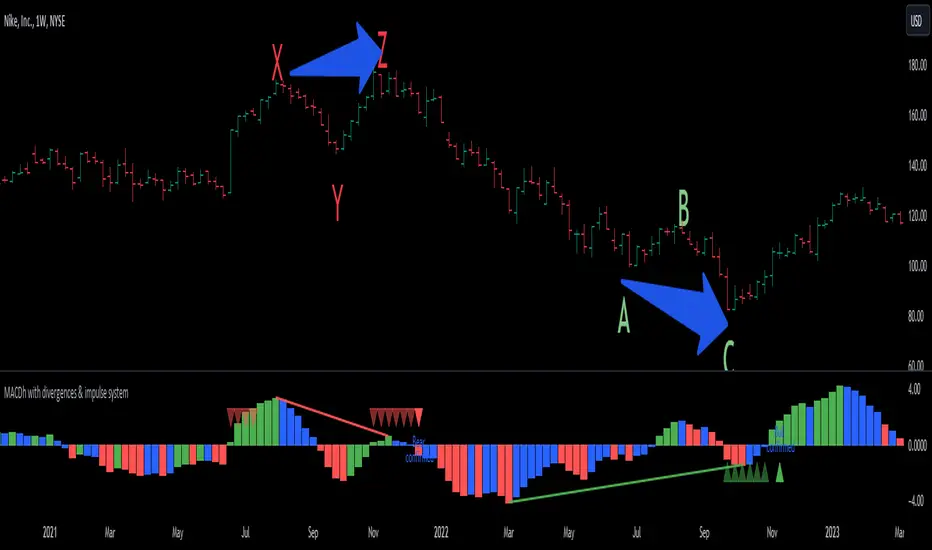
MACDh with divergences & impulse system (overlayed on prices)-----------------------------------------------------------------
General Description:
This indicator ( the one on the top panel above ) consists on some lines, arrows and labels drawn over the price bars/candles indicating the detection of regular divergences between price and the classic MACD histogram (shown on the low panel). This script is special because it can be adjusted to fit several criteria when trading divergences filtering them according to the "height" and "width" of the patterns. The script also includes the "extra features" Impulse System and Keltner Channels, which you will hardly find anywhere else in similar classic MACD histogram divergence indicators.
The indicator helps to find trend reversals, and it works on any market, any instrument, any timeframe, and any market condition (except against really strong trends that do not show any other sign of reversion yet).
Please take on consideration that divergences should be taken with caution.
-----------------------------------------------------------------
Definition of classic Bullish and Bearish divergences:
* Bearish divergences occur in uptrends identifying market tops. A classical or regular bearish divergence occurs when prices reach a new high and then pull back, with an oscillator (MACD histogram in this case) dropping below its zero line. Prices stabilize and rally to a higher high, but the oscillator reaches a lower peak than it did on a previous rally.
In the chart above (weekly charts of NKE, Nike, Inc.), in area X (around August 2021), NKE rallied to a new bull market high and MACD-Histogram rallied with it, rising above its previous peak and showing that bulls were extremely strong. In area Y, MACD-H fell below its centerline and at the same time prices punched below the zone between the two moving averages. In area Z, NKE rallied to a new bull market high, but the rally of MACD-H was feeble, reflecting the bulls’ weakness. Its downtick from peak Z completed a bearish divergence, giving a strong sell signal and auguring a nasty bear market.
* Bullish divergences , in the other hand, occur towards the ends of downtrends identifying market bottoms. A classical (also called regular) bullish divergence occurs when prices and an oscillator (MACD histogram in this case) both fall to a new low, rally, with the oscillator rising above its zero line, then both fall again. This time, prices drop to a lower low, but the oscillator traces a higher bottom than during its previous decline.
In the example in the chart above (weekly charts of NKE, Nike, Inc.), you see a bearish divergence that signaled the October 2022 bear market bottom, giving a strong buy signal right near the lows. In area A, NKE (weekly charts) appeared in a free fall. The record low A of MACD-H indicated that bears were extremely strong. In area B, MACD-H rallied above its centerline. Notice the brief rally of prices at that moment. In area C, NKE slid to a new bear market low, but MACD-H traced a much more shallow low. Its uptick completed a bullish divergence, giving a strong buy signal.
-----------------------------------------------------------------
Some cool features included in this indicator:
1. This indicator also includes the “ Impulse System ”. The Impulse System is based on two indicators, a 13-day exponential moving average and the MACD-Histogram, and identifies inflection points where a trend speeds up or slows down. The moving average identifies the trend, while the MACD-Histogram measures momentum. This unique indicator combination is color coded into the price bars for easy reference.
Calculation:
Green Price Bar: (13-period EMA > previous 13-period EMA) and
(MACD-Histogram > previous period's MACD-Histogram)
Red Price Bar: (13-period EMA < previous 13-period EMA) and
(MACD-Histogram < previous period's MACD-Histogram)
Price bars are colored blue when conditions for a Red Price Bar or Green Price Bar are not met. The MACD-Histogram is based on MACD(12,26,9).
The Impulse System works more like a censorship system. Green price bars show that the bulls are in control of both trend and momentum as both the 13-day EMA and MACD-Histogram are rising (you don't have permission to sell). A red price bar indicates that the bears have taken control because the 13-day EMA and MACD Histogram are falling (you don't have permission to buy). A blue price bar indicates mixed technical signals, with neither buying nor selling pressure predominating (either both buying or selling are permitted).
2. Another "extra feature" included here is the " Keltner Channels ". Keltner Channels are volatility-based envelopes set above and below an exponential moving average.
3. It were also included a couple of EMAs.
Everything can be removed from the chart any time.
-----------------------------------------------------------------
Options/adjustments for this indicator:
*Horizontal Distance (width) between two tops/bottoms criteria.
Refers to the horizontal distance between the MACH histogram peaks involved in the divergence
*Height of tops/bottoms criteria (for Histogram).
Refers to the difference/relation/vertical distance between the MACH HISTOGRAM peaks involved in the divergence: 1st Histogram Peak is X times the 2nd.
*Height/Vertical deviation of tops/bottoms criteria (for Price).
Deviation refers to the difference/relation/vertical distance between the PRICE peaks involved in the divergence.
*Plot Regular Bullish Divergences?.
*Plot Regular Bearish Divergences?.
*Delete Previous Cancelled Divergences?.
*Shows a pair of EMAs.
*Shows Keltner Channels (using ATR)
Keltner Channels are volatility-based envelopes set above and below an exponential moving average.
*This indicator also has the option to show the Impulse System over the price bars/candles.
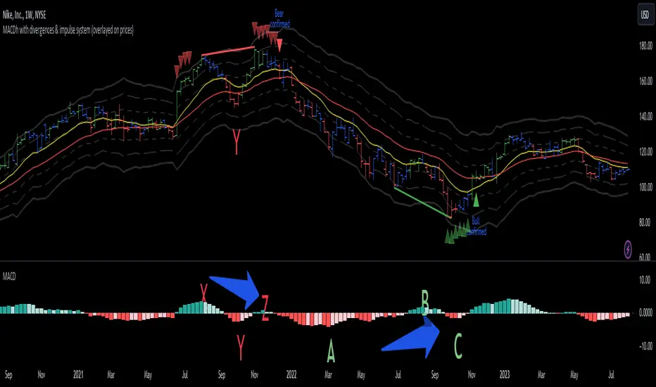
MACDh with divergences & impulse system-----------------------------------------------------------------
General Description:
This indicator ( the one on the low panel ) is a classic MACD that also shows regular divergences between its histogram and the prices. This script is special because it can be adjusted to fit several criteria when trading divergences filtering them according to the "height" and "width" of the patterns. The script also includes the "extra feature" Impulse System, which you will hardly find anywhere else in similar classic MACD histogram divergence indicators.
The indicator helps to find trend reversals, and it works on any market, any instrument, any timeframe, and any market condition (except against really strong trends that do not show any other sign of reversion yet).
Please take on consideration that divergences should be taken with caution.
-----------------------------------------------------------------
Definition of classic Bullish and Bearish divergences:
* Bearish divergences occur in uptrends identifying market tops. A classical or regular bearish divergence occurs when prices reach a new high and then pull back, with an oscillator (MACD histogram in this case) dropping below its zero line. Prices stabilize and rally to a higher high, but the oscillator reaches a lower peak than it did on a previous rally.
In the chart above (weekly charts of NKE, Nike, Inc.), in area X (around August 2021), NKE rallied to a new bull market high and MACD-Histogram rallied with it, rising above its previous peak and showing that bulls were extremely strong. In area Y, MACD-H fell below its centerline and at the same time prices punched below the zone between the two moving averages. In area Z, NKE rallied to a new bull market high, but the rally of MACD-H was feeble, reflecting the bulls’ weakness. Its downtick from peak Z completed a bearish divergence, giving a strong sell signal and auguring a nasty bear market.
* Bullish divergences , in the other hand, occur towards the ends of downtrends identifying market bottoms. A classical (also called regular) bullish divergence occurs when prices and an oscillator (MACD histogram in this case) both fall to a new low, rally, with the oscillator rising above its zero line, then both fall again. This time, prices drop to a lower low, but the oscillator traces a higher bottom than during its previous decline.
In the example in the chart above (weekly charts of NKE, Nike, Inc.), you see a bearish divergence that signaled the October 2022 bear market bottom, giving a strong buy signal right near the lows. In area A, NKE (weekly charts) appeared in a free fall. The record low A of MACD-H indicated that bears were extremely strong. In area B, MACD-H rallied above its centerline. Notice the brief rally of prices at that moment. In area C, NKE slid to a new bear market low, but MACD-H traced a much more shallow low. Its uptick completed a bullish divergence, giving a strong buy signal.
-----------------------------------------------------------------
Extra feature: Impulse System
This indicator also includes the “ Impulse System ”. The Impulse System is based on two indicators, a 13-day exponential moving average and the MACD-Histogram, and identifies inflection points where a trend speeds up or slows down. The moving average identifies the trend, while the MACD-Histogram measures momentum. This unique indicator combination is color coded into the price bars or macd histogram bars for easy reference.
Calculation:
Green Price Bar: (13-period EMA > previous 13-period EMA) and
(MACD-Histogram > previous period's MACD-Histogram)
Red Price Bar: (13-period EMA < previous 13-period EMA) and
(MACD-Histogram < previous period's MACD-Histogram)
Histogram bars are colored blue when conditions for a Red Histogram Bar or Green Histogram Bar are not met. The MACD-Histogram is based on MACD(12,26,9).
The Impulse System works more like a censorship system. Green histogram bars show that the bulls are in control of both trend and momentum as both the 13-day EMA and MACD-Histogram are rising (you don't have permission to sell). A red histogram bar indicates that the bears have taken control because the 13-day EMA and MACD Histogram are falling (you don't have permission to buy). A blue histogram bar indicates mixed technical signals, with neither buying nor selling pressure predominating (either both buying or selling are permitted).
The impulse system can be removed from the chart any time.
-----------------------------------------------------------------
Options/adjustments for this indicator:
*Horizontal Distance (width) between two tops/bottoms criteria.
Refers to the horizontal distance between the MACH histogram peaks involved in the divergence
*Height of tops/bottoms criteria (for Histogram).
Refers to the difference/relation/vertical distance between the MACH HISTOGRAM peaks involved in the divergence: 1st Histogram Peak is X times the 2nd.
*Height/Vertical deviation of tops/bottoms criteria (for Price).
Deviation refers to the difference/relation/vertical distance between the PRICE peaks involved in the divergence.
*Plot Regular Bullish Divergences?.
*Plot Regular Bearish Divergences?.
*Delete Previous Cancelled Divergences?.
*This indicator also has the option to show the Impulse System over the MACD histogram bars
CC Trend strategy 2- Downtrend ShortTrend Strategy #2
Indicators:
1. EMA(s)
2. Fibonacci retracement with a mutable lookback period
Strategy:
1. Short Only
2. No preset Stop Loss/Take Profit
3. 0.01% commission
4. When in a profit and a closure above the 200ema, the position takes a profit.
5. The position is stopped When a closure over the (0.764) Fibonacci ratio occurs.
* NO IMMEDIATE RE-ENTRIES EVER!*
How to use it and what makes it unique:
This strategy will enter often and stop quickly. The goal with this strategy is to take losses often but catch the big move to the downside when it occurs through the Silvercross/Fibonacci combination. This is a unique strategy because it uses a programmed Fibonacci ratio that can be used within the strategy and on any program. You can manipulate the stats by changing the lookback period of the Fibonacci retracement and looking at different assets/timeframes.
This description tells the indicators combined to create a new strategy, with commissions and take profit/stop loss conditions included, and the process of strategy execution with a description of how to use it. If you have any questions feel free to PM me and boost if you found it helpful. Thank you, pineUSERS!
CHEATCODE1

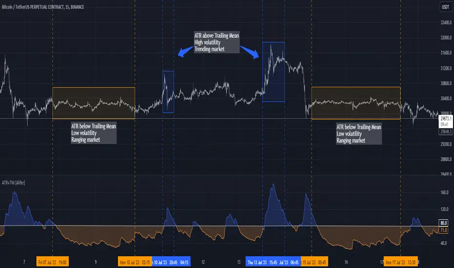
Average True Range Trailing Mean [Alifer]Upgrade of the Average True Range default indicator by TradingView. It adds and plots a trailing mean to show periods of increased volatility more clearly.
ATR TRAILING MEAN
A trailing mean, also known as a moving average, is a statistical calculation used to smooth out data over time and identify trends or patterns in a time series.
In our indicator, it clearly shows when the ATR value spikes outside of it's average range, making it easier to identify periods of increased volatility.
Here's how the ATR Trailing Mean (atr_mean) is calculated:
atr_mean = ta.cum(atr) / (bar_index + 1) * atr_mult
The ta.cum() function calculates the cumulative sum of the ATR over all bars up to the current bar.
(bar_index + 1) represents the number of bars processed up to the current bar, including the current one.
By dividing the cumulative ATR ta.cum(atr) by (bar_index + 1) and then multiplying it by atr_mult (Multiplier), we obtain the ATR Trailing Mean value.
If atr_mult is set to 1.0, the ATR Trailing Mean will be equal to the simple average of the ATR values, and it will follow the ATR's general trend.
However, if atr_mult is increased, the ATR Trailing Mean will react more strongly to the ATR's recent changes, making it more sensitive to short-term fluctuations.
On the other hand, reducing atr_mult will make the ATR Trailing Mean less responsive to recent changes in ATR, making it smoother and less prone to reacting to short-term volatility.
In summary, adjusting the atr_mult input allows traders to fine-tune the ATR Trailing Mean's responsiveness based on their preferred level of sensitivity to recent changes in market volatility.
IMPLEMENTATION IN A STRATEGY
You can easily implement this indicator in an existing strategy, to only enter positions when the ATR is above the ATR Trailing Mean (with Multiplier-adjusted sensitivity). To do so, add the following lines of codes.
Under Inputs:
length = input.int(title="Length", defval=20, minval=1)
atr_mult = input.float(defval=1.0, step = 0.1, title = "Multiplier", tooltip = "Adjust the sensitivity of the ATR Trailing Mean line.")
smoothing = input.string(title="Smoothing", defval="RMA", options= )
ma_function(source, length) =>
switch smoothing
"RMA" => ta.rma(source, length)
"SMA" => ta.sma(source, length)
"EMA" => ta.ema(source, length)
=> ta.wma(source, length)
This will allow you to define the Length of the ATR (lookback length over which the ATR is calculated), the Multiplier to adjust the Trailing Mean's sensitivity and the type of Smoothing to be used for the ATR.
Under Calculations:
atr= ma_function(ta.tr(true), length)
atr_mean = ta.cum(atr) / (bar_index+1) * atr_mult
This will calculate the ATR based on Length and Smoothing, and the resulting ATR Trailing Mean.
Under Entry Conditions, add the following to your existing conditions:
and atr > atr_mean
This will make it so that entries are only triggered when the ATR is above the ATR Trailing Mean (adjusted by the Multiplier value you defined earlier).
ATR - DEFINITION AND HISTORY
The Average True Range (ATR) is a technical indicator used to measure market volatility, regardless of the direction of the price. It was developed by J. Welles Wilder and introduced in his book "New Concepts in Technical Trading Systems" in 1978. ATR provides valuable insights into the degree of price movement or volatility experienced by a financial asset, such as a stock, currency pair, commodity, or cryptocurrency, over a specific period.
ATR - CALCULATION AND USAGE
The ATR calculation involves three components:
1 — True Range (TR): The True Range is a measure of the asset's price movement for a given period. It takes into account the following factors:
The difference between the high and low prices of the current period.
The absolute value of the difference between the high price of the current period and the closing price of the previous period.
The absolute value of the difference between the low price of the current period and the closing price of the previous period.
Mathematically, the True Range (TR) for the current period is calculated as follows:
TR = max(high - low, abs(high - previous_close), abs(low - previous_close))
2 — ATR Calculation: The ATR is calculated as a Moving Average (MA) of the True Range over a specified period.
The ATR is calculated as follows:
ATR = MA(TR, length)
3 — ATR Interpretation: The ATR value represents the average volatility of the asset over the chosen period. Higher ATR values indicate higher volatility, while lower ATR values suggest lower volatility.
Traders and investors can use ATR in various ways:
Setting Stop Loss and Take Profit Levels: ATR can help determine appropriate stop-loss and take-profit levels in trading strategies. A larger ATR value might require wider stop-loss levels to allow for the asset's natural price fluctuations, while a smaller ATR value might allow for tighter stop-loss levels.
Identifying Market Volatility: A sharp increase in ATR might indicate heightened market uncertainty or the potential for significant price movements. Conversely, a decreasing ATR might suggest a period of low volatility and possible consolidation.
Comparing Volatility Between Assets: Since ATR uses absolute values, it shouldn't be used to compare volatility between different assets, as assets with higher prices will consistently have higher ATR values, while assets with lower prices will consistently have lower ATR values. However, the addition of a trailing mean makes such a comparison possible. An asset whose ATR is consistently close to its ATR Trailing Mean will have a lower volatility than an asset whose ATR continuously moves far above and below its ATR Trailing Mean. This can help traders and investors decide which markets to trade based on their risk tolerance and trading strategies.
Determining Position Size: ATR can be used to adjust position sizes, taking into account the asset's volatility. Smaller position sizes might be appropriate for more volatile assets to manage risk effectively.
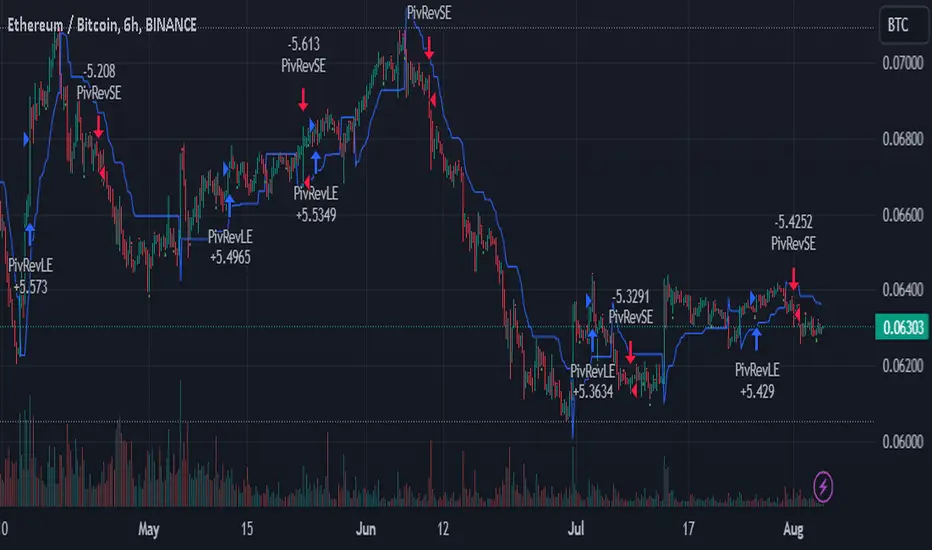
SuperTrend Enhanced Pivot Reversal - Strategy [PresentTrading]
- Introduction and How it is Different
The SuperTrend Enhanced Pivot Reversal is a unique approach to trading that combines the best of two worlds: the precision of pivot reversal points and the trend-following power of the SuperTrend indicator. This strategy is designed to provide traders with clear entry and exit points, while also filtering out potentially false signals using the SuperTrend indicator.
BTCUSDT 6hr
ETHBTC 6hr
Unlike traditional pivot reversal strategies, this approach uses the SuperTrend indicator as a filter. This means that it only takes trades that align with the overall trend, as determined by the SuperTrend indicator. This can help to reduce the number of false signals and improve the overall profitability of the strategy.
The Pivot Reversal Strategy with SuperTrend Filter is particularly well-suited to the cryptocurrency market for the reason of High Volatility. This means that prices can change rapidly in a very short time, making it possible to make a profit quickly. The strategy's use of pivot points allows traders to take advantage of these rapid price changes by identifying potential reversal points
- Strategy: How it Works
The strategy works by identifying pivot reversal points, which are points in the price chart where the price is likely to reverse. These points are identified using a combination of the ta.pivothigh and ta.pivotlow functions, which find the highest and lowest points in the price chart over a certain period.
Once a pivot reversal point is identified, the strategy checks the direction of the SuperTrend indicator. If the SuperTrend is positive (indicating an uptrend), the strategy will only take long trades. If the SuperTrend is negative (indicating a downtrend), the strategy will only take short trades.
The strategy also includes a stop loss level, which is set as a percentage of the entry price. This helps to limit potential losses if the price moves in the opposite direction to the trade.
- Trade Direction
The trade direction can be set to "Long", "Short", or "Both". This allows the trader to choose whether they want to take only long trades (buying low and selling high), only short trades (selling high and buying low), or both. This can be useful depending on the trader's view of the market and their risk tolerance.
- Usage
To use the Pivot Reversal Strategy with SuperTrend Filter, simply input the desired parameters into the script and apply it to the price chart of the asset you wish to trade. The strategy will then identify potential trade entry and exit points, which will be displayed on the price chart.
- Default Settings
The default settings for the strategy are as follows:
ATR Length: 5
Factor: 2.618
Trade Direction: Both
Stop Loss Level: 20%
Commission: 0.1%
Slippage: 1
Currency: USD
Each trade: 10% of account equity
Initial capital: $10,000
These settings can be adjusted to suit the trader's preferences and risk tolerance. Always remember to test any changes to the settings using historical data before applying them to live trades.
Developing Market Profile / TPO [Honestcowboy]The Developing Market Profile Indicator aims to broaden the horizon of Market Profile / TPO research and trading. While standard Market Profiles aim is to show where PRICE is in relation to TIME on a previous session (usually a day). Developing Market Profile will change bar by bar and display PRICE in relation to TIME for a user specified number of past bars.
What is a market profile?
"Market Profile is an intra-day charting technique (price vertical, time/activity horizontal) devised by J. Peter Steidlmayer. Steidlmayer was seeking a way to determine and to evaluate market value as it developed in the day time frame. The concept was to display price on a vertical axis against time on the horizontal, and the ensuing graphic generally is a bell shape--fatter at the middle prices, with activity trailing off and volume diminished at the extreme higher and lower prices."
For education on market profiles I recommend you search the net and study some profitable traders who use it.
Key Differences
Does not have a value area but distinguishes each column in relation to the biggest column in percentage terms.
Updates bar by bar
Does not take sessions into account
Shows historical values for each bar
While there is an entire education system build around Market Profiles they usually focus on a daily profile and in some cases how the value area develops during the day (there are indicators showing the developing value area).
The idea of trading based on a developing value area is what inspired me to build the Developing Market Profile.
🟦 CALCULATION
Think of this Developing Market Profile the same way as you would think of a moving average. On each bar it will lookback 200 bars (or as user specified) and calculate a Market Profile from those bars (range).
🔹Market Profile gets calculated using these steps:
Get the highest high and lowest low of the price range.
Separate that range into user specified amount of price zones (all spaced evenly)
Loop through the ranges bars and on each bar check in which price zones price was, then add +1 to the zones price was in (we do this using the OccurenceArray)
After it looped through all bars in the range it will draw columns for each price zone (using boxes) and make them as wide as the OccurenceArray dictates in number of bars
🔹Coloring each column:
The script will find the biggest column in the Profile and use that as a reference for all other columns. It will then decide for each column individually how big it is in % compared to the biggest column. It will use that percentage to decide which color to give it, top 20% will be red, top 40% purple, top 60% blue, top 80% green and all the rest yellow. The user is able to adjust these numbers for further customisation.
The historical display of the profiles uses plotchar() and will not only use the color of the column at that time but the % rating will also decide transparancy for further detail when analysing how the profiles developed over time. Each of those historical profiles is calculated using its own 200 past bars. This makes the script very heavy and that is why it includes optimisation settings, more info below.
🟦 USAGE
My general idea of the markets is that they are ever changing and that in studying that changing behaviour a good trader is able to distinguish new behaviour from old behaviour and adapt his approach before losing traders "weak hands" do.
A Market Profile can visually show a trader what kind of market environment we currently are in. In training this visual feedback helps traders remember past market environments and how the market behaved during these times.
Use the history shown using plotchars in colors to get an idea of how the Market Profile looked at each bar of the chart.
This history will help in studying how price moves at different stages of the Market Profile development.
I'm in no way an expert in trading Market Profiles so take this information with a grain of salt. Below an idea of how I would trade using this indicator:
🟦 SETTINGS
🔹MARKET PROFILING
Lookback: The amount of bars the Market Profile will look in the past to calculate where price has been the most in that range
Resolution: This is the amount of columns the Market Profile will have. These columns are calculated using the highest and lowest point price has been for the lookback period
Resolution is limited to a maximum of 32 because of pinescript plotting limits (64). Each plotchar() because of using variable colors takes up 2 of these slots
🔹VISUAL SETTINGS
Profile Distance From Chart: The amount of bars the market profile will be offset from the current bar
Border width (MP): The line thickness of the Market Profile column borders
Character: This is the character the history will use to show past profiles, default is a square.
Color theme: You can pick 5 colors from biggest column of the Profile to smallest column of the profile.
Numbers: these are for % to decide column color. So on default top 20% will be red, top 40% purple... Always use these in descending order
Show Market Profile: This setting will enable/disable the current Market Profile (columns on right side of current bar)
Show Profile History: This setting will enable/disable the Profile History which are the colored characters you see on each bar
🔹OPTIMISATION AND DEBUGGING
Calculate from here: The Market Profile will only start to calculate bar by bar from this point. Setting is needed to optimise loading time and quite frankly without it the script would probably exceed tradingview loading time limits.
Min Size: This setting is there to avoid visual bugs in the script. Scaling the chart there can be issues where the Market Profile extends all the way to 0. To avoid this use a minimum size bigger than the bugged bottom box
Pivot HL Trading SetupThis simple script base on function of Pivot High Low to plot Trading Setup on chart with detail as below:
2. Trading Setup
2.1 Buy setup
+ New Pivot Low is plotted
+ Entry Long at market price.
+ Stoploss at Pivot Low
+ Takeprofit at Pivot High
+ Buy setup invalidation when price crossed Pivot High or Pivot Low
2.1 Sell setup
+ New Pivot High is plotted
+ Entry Short at market price.
+ Stoploss at Pivot High
+ Takeprofit at Pivot Low
+ Sell setup invalidation when price crossed Pivot High or Pivot Low

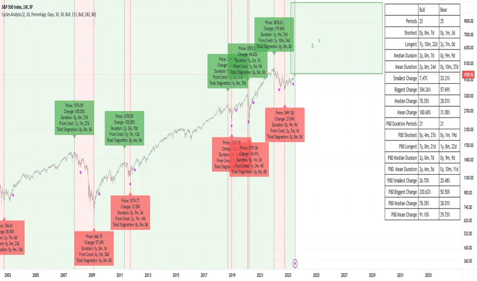
Cycles AnalysisI strongly believe in cycles, so I wanted to create something that would give a visual representation of bull/bear markets and give a prediction based on the previous data. It's up to you how to decide what is a bull/bear cycle. There is no single rule for all assets because 20% drop in SP500 starts a bear market in traditional markets, while 35% drop for Bitcoin is a Tuesday. You have two options on how to decide when markets turn: either by a % change (traditional definition) or if there is no new high/low after X days. A softer version to show periods of no new highs/lows is to use the Stagnation option. Stagnation periods hava the same logic as the cycle change by X days: if there is no new high/low then we treat this period as a stagnation. The difference is that stagnation periods do not change cycle directions and do not participate in calculations.
The script also draws a possible "predictions" zone where the current cycle might end up. There is no magic here, it just takes previous cycles' size to draw the possible boundaries. If you decide to use percentiles then the box area will be taken from the percentiles calculations, otherwise it will come from the full data. "x" in the predictions zone represents a target mean (average) value, "o" represents a target median value.
A few things to keep in mind:
- this script is not supposed to be used in trading. It was created for analysis. It repaints. And when I say "it repaints" - it might like repaint the last 6 months of data if a new low comes and we are in a stagnation period (aka not a financial advice).
- it doesn't work with replays as it does calculations only once on the last candle.
- you need at least 3 periods to be able to calculate percentiles. And after this it will remove at least 1 period on each side. Which means that 90 percentile will not be a real 90 percentile until you have enough periods for it to be (20 in this specific case).
- it assumes that a year = 360 days, and a month = 30 days. So the duration presentation might not be exact, until you move to the day level.
- I had macro analysis in mind when I created the script, but nothing stops you from using it in a 1m time frame for BTC. Just change the time duration presentation.
- the last period is not finished, so it doesn't participate in calculations.
VOLD Ratio (Volume Difference Ratio) by TenozenAnother helpful indicator is here! VOLD Ratio is calculated by the net volume of a buying candle, divided by the net volume of a sell candle.
Formula:
buying net volume/selling net volume
It's a simple indicator, but don't underestimate this simplicity. It's a powerful indicator that would help you to decide whether the volume is getting interested in the direction that the market would take. So assume when the market is above the Bollinger Bands, it means that the volume is at a buying extreme, by that, we could expect the market to get back towards the mean, as there is a lot of buying demand that entered the market. How about below the Bollinger Bands? it means that the volume is at a selling extreme, we could expect that there is a lot of volume getting in toward the sellers, so we could take advantage of the opportunity to go for a long. Lastly, the Bollinger Bands would help you guys to determine the liquidity of the market, if the Bollinger Bands get smaller over time, it means there is no interest for the market to enter yet, and if the Bollinger Bands get bigger over time, it means there is interest for the market to enter in the session.
Tips & Reminder:
- We shouldn't use this indicator by itself, make sure to use an Indicator that would help you guys to determine the momentum and the liquidity of the market.
- The higher the timeframe, the slower this indicator would signal an entry, by that use a smaller timeframe... I suggest using a 15M chart for the execution.
- Always trade in the medium-longterm direction if you want to have a high probability trade.
- Be patient in your execution, it's more likely the market would go higher or lower after going in the extreme of the Bollinger Bands.
Well, that's it! Hope you guys enjoy using this indicator, let me know if there is any question or suggestion. Ciao...

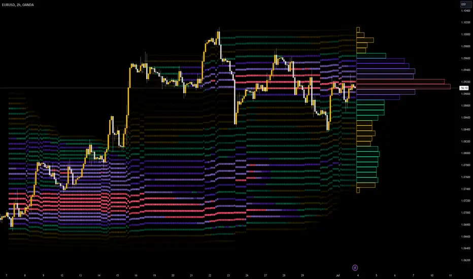
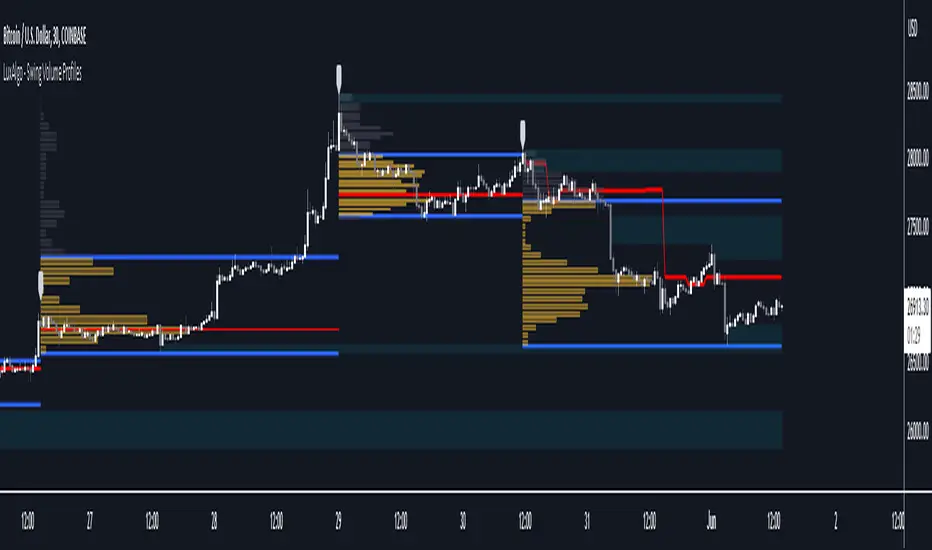
Swing Volume Profiles [LuxAlgo]The Swing Volume Profiles indicator aims to calculate and highlight trading activity at specific price levels between two swing points; allowing traders to reveal dominant and/or significant price levels based on volume.
By measuring traded volume at all price levels in the market over a specified time period, the script can also be used to detect some key analysis generally such as supply & demand, buy-side & sell-side liquidity levels, unfilled liquidity voids, and imbalances that can highlight on the chart.
🔶 USAGE
A volume profile is an advanced charting tool that displays the traded volume at different price levels over a specific period. It helps you visualize where the majority of trading activity has occurred.
Key Levels are the areas where the volume is concentrated or where there are significant volume spikes. These levels are known as key support and resistance levels. High-volume nodes indicate areas of high activity and are likely to act as support or resistance in the future.
Volume profile also helps identify value areas, which represent the price levels where the most trading activity has taken place. These levels can act as areas of support or resistance as traders perceive them as fair value.
The Point of Control describes the price level where the most volume was traded. A Naked Point of Control (also called a Virgin Point of Control) is a previous POC that has not been traded. Extending PoC options 'Until Bar Cross' or 'Until Bar Touch' helps in identifying Naked Point of Control Lines.
Previous PoC levels can serve as support and resistance for future price movements. Extending PoC Level 'Until Last Bar' option will help to identify such levels.
🔶 DETAILS
One of the unique features of the script is its ability to detect some other key levels such as levels of acceptance and rejection.
Levels of rejection we may summarize as supply and demand levels, these are also referred to as buy-side and sell-side liquidity levels. They usually occur at extreme highs or lows, where prices may be too high for buyers (high supply, low demand) or too low for sellers (low supply, high demand)
Levels of acceptance are the levels where Liquidity Voids occur, these are also referred to imbalances. Liquidity voids are sudden changes in price when the price jumps from one level to another. The peculiar thing about liquidity voids is that they almost always fill up, so we call them levels of acceptance.
🔶 ALERTS
When an alert is configured, the user will have the ability to be notified in case:
Point Of Control Line is touched/crossed
Value Area High Line is touched/crossed
Value Area Low Line is touched/crossed
🔶 SETTINGS
🔹 Display Options
Mode: Controls the lookback length of detection and visualization, where Present assumes last X bars specifid in '# Bars' option and Historical assumes all data available to the user as well as allowed limits of visiual objects (boxs, lines, labels etc)
# Bars: Controls the lookback length.
🔹 Swing Volume Profiles
The script takes into account user-defined parameters and plots volume profiles. Due to Pine Script™ drwaing objects limit only total volume profiles are presented.
Swing Detection Length: Lookback period
Swing Volume Profiles: Toggles the visibility of the Volume Profiles, with color options to differentiate the Value Area within a profile.
Profile Range Background Fill: Toggles the visibility of the Volume Profiles Range
🔹 Point of Control (PoC)
Point of Control (POC) – The price level for the time period with the highest traded volume
Point of Control (PoC): Toggles the visibility of the Point of Control
Developing PoC: Toggles the visibility of the Developing PoC
Extend PoC: Option that allows detecting virgin PoC levels. Virgin Point of Control (VPoC) is defined as a Point of Control that has never been revisited or touched. The option also allows PoC levels to extend till the last bar aiming to present levels from history where the levels were traded significantly and those levels can be used as support and resistance levels.
🔹 Value Area (VA)
Value Area (VA) – The range of price levels in which the specified percentage of all volume was traded during the time period.
Value Area Volume %: Specifies percentage of the Value Area
Value Area High (VAH): Toggles the visibility of the Value Area High, the highest price level within the Value Area
Value Area Low (VAL): Toggles the visibility of the Value Area Low, the lowest price level within the Value Area
Value Area (VA) Background Fill: Toggles the visibility of the Value Area Range
🔹 Liquidity Levels / Voids
Unfilled Liquidity, Thresh: Enable display of the Unfilled Liquidity Levels and Liquidity Voids, where threshold value defines the significance of the level.
🔹 Profile Stats
Position, Size: Specifies the position and the size of the label presenting Profile Stats, the tooltip of the label includes all related info for each profile.
Price, Price Change, and Cumulative Volume: Enable display of the given options on the chart.
🔹 Volume Profile Others
Number of Rows: Specify how many rows each histogram will have. Caution, having it set to high values will quickly hit Pine Script™ drawing objects limit and may cause fewer historical profiles to be displayed.
Placement: Place profile either left or right.
Profile Width %: Alters the width of the rows in the histogram, relative to the calculated profile length.
🔶 RELATED SCRIPTS
Alternative Liquidity Void Detection script, Buyside-Sellside-Liquidity
RSI of Zero Lag MA (ValueRay)The RSI of a Zero Lag Moving Average a powerful tool for for reliable exit signals.
The Relative Strength Index (RSI) is a widely recognized momentum oscillator that measures the speed and change of price movements. It provides valuable insights into overbought and oversold conditions, enabling traders to identify potential reversal points and take advantage of market inefficiencies.
The RSI of a Zero Lag Indicator takes this concept a step further by incorporating the Zero Lag Moving Average. The Zero Lag Moving Average is a cutting-edge indicator that minimizes lag and provides a smoother representation of price action, allowing for quicker and more precise responses to market movements.
By combining the RSI with the Zero Lag Moving Average, this indicator offers traders a superior exit strategy. When the RSI reaches extreme levels of overbought or oversold conditions, it indicates a potential reversal in the market. The Zero Lag Moving Average further enhances this signal by reducing delays and providing timely exit points.
Moreover, the RSI of a Zero Lag Indicator is not limited to mean reversion strategies. While it excels in identifying mean reversion opportunities, it can also be used in conjunction with other trading approaches. Traders can take advantage of its objective signals to exit trades profitably, regardless of their chosen strategy.
With its ability to accurately pinpoint overbought and oversold conditions, the RSI of a Zero Lag Indicator offers traders a competitive edge in the market. By providing timely exit signals and minimizing lag, it helps traders optimize their trading decisions and increase their chances of success.

Mad_StandardpartsLibrary "Mad_Standardparts"
This are my Standardparts used in upcoming scipts
roundTo(_value, _decimals)
Round a floating point value to a specified number of decimal places.
@description This function takes a floating point value and rounds it to a specified number of decimal places.
Parameters:
_value (float) : The floating point value to be rounded.
_decimals (int) : The number of decimal places to round to. Must be a non-negative integer.
Returns: The rounded value, as a floating point number.
clear_all()
Delete all drawings on the chart.
@description This function deletes all drawings on the chart, including lines, boxes, and labels.
Returns: None.
shifting(_value)
Create a string of spaces to shift text over by a specified amount.
@description This function takes an integer value and returns a string consisting of that many spaces, which can be used to shift text over in a PineScript chart.
Parameters:
_value (int) : The number of spaces to create in the output string.
Returns: A string consisting of the specified number of spaces.
fromLog(_value)
Convert a linear value to a logarithmic value.
@description This function takes a linear value and converts it to a logarithmic value, using the formula specified in the code.
Parameters:
_value (float)
Returns: The corresponding logarithmic value, as a floating point number.
toLog(_value)
Convert a logarithmic value to a linear value.
@description This function takes a logarithmic value and converts it to a linear value, using the formula specified in the code.
Parameters:
_value (float)
Returns: The corresponding linear value, as a floating point number.
f_getbartime()
Calculate the time per bar on the chart.
@description This function calculates the time per bar on the chart based on the first 100 bars.
Returns: The time per bar, as an integer value.

Volatility patterns / quantifytools- Overview
Volatility patterns detect various forms of indecisive price action, on a larger scale as a compressed range and on a smaller scale as indecision candles. Indecisive and volatility suppressing price action can be thought of as a spring being pressed down. The more suppression, the more tension is built and eventually released as a spike or series of spikes in volatility. Each volatility pattern is assigned an influence period, during which average and peak relative volatility is recorded and stored to volatility metrics.
- Patterns
The following scenarios are qualified as indecision candles: inside candles, indecision engulfing candles and volatility shifts.
By default, each indecision candle is considered a valid pattern only when another indecision candle has taken place within 3 periods, e.g. prior inside candle + indecision engulfing candle = valid volatility pattern. This measurement is taken to filter noise by looking for multiple hints of pending volatility, rather than just one. Level of tolerated noise can be changed via input menu by using sensitivity setting, by default set to 2.
Sensitivity at 1: Any single indecision candle is considered a valid pattern
Sensitivity at 2: 2 indecision candles within 3 bars is considered a valid pattern
Sensitivity at 3: 2 indecision candles within 2 bars (consecutive) is considered a valid pattern
The following scenarios are qualified as range patterns: series of lower highs/higher lows and series of low volatility pivots.
A pivot is defined by highest/lowest point in price, by default within 2 periods back and 2 periods forward. When 4 pivots with qualities mentioned above are found, a box indicating compressed range will appear. Both required pivots and pivot definition can be adjusted via input menu.
- Influence time and metrics
By default, influence time for each volatility pattern is set to 6 candles, a period for which spike(s) in volatility is expected. For each influence period, average relative volatility (volatility relative to volatility SMA 20) and peak relative volatility is recorded and stored to volatility metrics. All metrics used in calculations are visible in "Data Window "tab. Average and peak volatility during influence period will vary depending on chart, timeframe and chosen settings. Tweaking the settings might result in an improvement and is worth experimenting with.
- Visuals
By default, indecision candles are visualized as yellow lines and range patterns as orange boxes. Influence time periods are respectively visualized as colored candle borders, applied as long as influence time period is active. All colors are fully customizable via input menu.
- Practical guide
Volatility patterns depict moments of equal strength from both bulls and bears. While this equilibrium is in place, price is stagnant and compresses until either side initiates volatility, releasing the built up tension. On top of hedging and playing the volatility using volatility based instruments, some other methods can be applied to take advantage of the somewhat tricky areas of indecision.
Example #1: Trading volatility
Volatility is not a bad thing from a trading perspective, but can actually be fertile ground for executing trade setups. Trading volatility influence periods from higher timeframes on lower timeframes gives greater resolution to work with and opportunities to take advantage of the wild swings created.
Example #2: Finding bias for patterns
Points of confluence where it anyway makes sense to favor one side over the other can be used for establishing bias for indecisive price action as well. At face value, it makes sense to expect bearish reactions at range highs and bullish reactions at range low, for which volatility patterns can provide a catalyst.
Example #3: Betting on initiation direction
Betting on direction of the first volatile move can easily go against you, but if risk/reward is able to compensate for the poor win rate, it's a valid idea to consider and explore.