BanditExperimental %R and Moving Average Bands. This is just for fun :)
Comment below if you spot a good pattern to trade.
Search in scripts for "band"

ATR Overlay with Trailing Flip [ask2maniish]📘 ATR Overlay with Trailing Flip
🔍 Overview
The ATR Overlay with Trailing Flip is a dynamic, visually-enhanced overlay indicator designed to assist traders in trend detection, trailing stop management, and volatility-based decision making. It leverages the Average True Range (ATR) with optional dynamic multipliers, filters, and alerts to enhance trade execution precision.
⚙️ Features Summary
✅ Static & dynamic ATR multiplier
✅ Customizable trailing stop logic
✅ Volume & Bollinger Band filters
✅ Buy/Sell label signals with alerts
✅ ATR bands with color fill
✅ Optional candle coloring based on trend
✅ Table showing current ATR multiplier
✅ Fully customizable visual controls
🔧 User Inputs
📘 Info Panel
ATR Usage Guide
Tooltip with trading-style recommendations:
Scalping: ATR 5–10, Intraday: ATR 10–14 , Swing: ATR 14–21 , Position: ATR 21–50
📊 Visual Elements
📈 Plots
Upper/Lower ATR Bands
ATR Fill Zone
Dynamic Trailing Stop Line
🕯 Candle Coloring
Candles colored green (uptrend) or red (downtrend)
Wick coloring matches body
🏷 Signal Labels
"BUY" below candle when trend flips up
"SELL" above candle when trend flips down
📊 Table (Top Right)
Displays current multiplier value:
If static: Static: x.x
If dynamic: percentage format based on ATR ratio
🔔 Alerts
Two alert conditions:
Flip to Long → "📈 ATR flip to LONG"
Flip to Short → "📉 ATR flip to SHORT"
Sound can be enabled for real-time feedback.
🧠 Best Practices
Combine this tool with support/resistance or order flow indicators
Use dynamic ATR during volatile periods for better adaptability
Filter signals in ranging markets with BBand Width Filter
For scalping, reduce ATR period and multiplier for tighter risk
🛠️ Customization Tips
Adjust trailingPeriod for tighter/looser stops
Use color inputs to match your charting theme
Disable features (labels/fill) to declutter chart

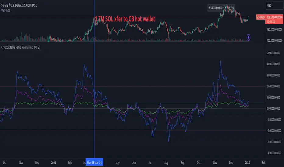
Crypto/Stable Mcap Ratio NormalizedCreate a normalized ratio of total crypto market cap to stablecoin supply (USDT + USDC + DAI). Idea is to create a reference point for the total market cap's position, relative to total "dollars" in the crypto ecosystem. It's an imperfect metric, but potentially helpful. V0.1.
This script provides four different normalization methods:
Z-Score Normalization:
Shows how many standard deviations the ratio is from its mean
Good for identifying extreme values
Mean-reverting properties
Min-Max Normalization:
Scales values between 0 and 1
Good for relative position within recent range
More sensitive to recent changes
Percent of All-Time Range:
Shows where current ratio is relative to all-time highs/lows
Good for historical context
Less sensitive to recent changes
Bollinger Band Position:
Similar to z-score but with adjustable sensitivity
Good for trading signals
Can be tuned via standard deviation multiplier
Features:
Adjustable lookback period
Reference bands for overbought/oversold levels
Built-in alerts for extreme values
Color-coded plots for easy visualization
PUBG//Pluto star appears on a chart when price goes in the in the extreme price range territory, i.e. beyond 2 standard deviation from the mean (or mid Bollinger Band).
//What makes a Pluto Star appear on a chart:
//1. Check if the candle 's' high and low, both are completely outside of the Bollinger Bands (close, 20, 2) - Lets call it Pluto Star Candle
//2. Pluto Star Candle must not be a result of sudden price movement. Hence the previous candle must give a BB Blast.
// In other words, the candle must have it's either open or close outside of Bollinger Bands, to confirm a BB Blast before the Pluto Star
//3. Candle, following the Pluto Star must not break the high (in case of upper BB i.e. short call) or low (in case of lower BB, i.e. long call), to confirm the reversal to the mean
// This implies that Pluto Star appears on chart, above/below the next candle of actual Pluto Star Candle

BTC Fair Value via Global Liquidity📈 BTC Fair Value via Global Liquidity
This indicator estimates Bitcoin's fair value based on a regression model using Global Liquidity (GLI) data from major central banks.
🔍 How it works:
Fair Value Line (orange): Calculated using a power-law model: Fair Value = e^b * (GLI)^a, where a and b are user-defined parameters based on historical regression.
Global Liquidity (GLI): Combines liquidity metrics from central banks (Fed, ECB, PBoC, BoJ, etc.), including adjustments for the RRP and TGA.
Deviation Bands (green/red dashed): Optional upper and lower bands showing % deviation from fair value (default ±25%). These help identify overbought/oversold conditions.
Delta Plot (gray dots): Displays the % deviation of BTC’s price from its modeled fair value.
⚙️ How to use:
Tune a and b for better model fitting (e.g., via log-log regression).
Use the deviation bands to identify potential entry/exit zones or periods of market inefficiency.
Ideal for macro-level BTC valuation and long-term strategic analysis.

Bollinger + EMA Strategy with StatsThis strategy is a mean-reversion trading model that combines Bollinger Band deviation entries with EMA-based exits. It enters a long position when the price drops significantly below the lower Bollinger Band by a user-defined multiple of standard deviation (x), and a short position when the price exceeds the upper band by the same logic. To manage risk, it uses a wider Bollinger Band threshold (y standard deviations) as a stop loss, while take profit occurs when the price reverts to the n-period EMA, indicating mean reversion. The strategy maintains only one active position at a time—either long or short—and allocates a fixed percentage of capital per trade. Performance metrics such as equity curve, drawdown, win rate, and total trades are tracked and displayed for backtesting evaluation.

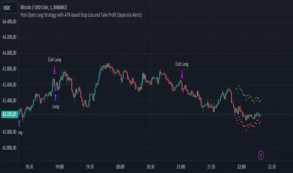
Post-Open Long Strategy with ATR-based Stop Loss and Take ProfitThe "Post-Open Long Strategy with ATR-Based Stop Loss and Take Profit" is designed to identify buying opportunities after the German and US markets open. It combines various technical indicators to filter entry signals, focusing on breakout moments following price lateralization periods.
Key Components and Their Interaction:
Bollinger Bands (BB):
Description: Uses BB with a 14-period length and standard deviation multiplier of 1.5, creating narrower bands for lower timeframes.
Role in the Strategy: Identifies low volatility phases (lateralization). The lateralization condition is met when the price is near the simple moving average of the BB, suggesting an imminent increase in volatility.
Exponential Moving Averages (EMA):
10-period EMA: Quickly detects short-term trend direction.
200-period EMA: Filters long-term trends, ensuring entries occur in a bullish market.
Interaction: Positions are entered only if the price is above both EMAs, indicating a consolidated positive trend.
Relative Strength Index (RSI):
Description: 7-period RSI with a threshold above 30.
Role in the Strategy: Confirms the market is not oversold, supporting the validity of the buy signal.
Average Directional Index (ADX):
Description: 7-period ADX with 7-period smoothing and a threshold above 10.
Role in the Strategy: Assesses trend strength. An ADX above 10 indicates sufficient momentum to justify entry.
Average True Range (ATR) for Dynamic Stop Loss and Take Profit:
Description: 14-period ATR with multipliers of 2.0 for Stop Loss and 4.0 for Take Profit.
Role in the Strategy: Adjusts exit levels based on current volatility, enhancing risk management.
Resistance Identification and Breakout:
Description: Analyzes the highs of the last 20 candles to identify resistance levels with at least two touches.
Role in the Strategy: A breakout above this level signals a potential continuation of the bullish trend.
Time Filters and Market Conditions:
Trading Hours: Operates only during the opening of the German market (8:00 - 12:00) and US market (15:30 - 19:00).
Panic Candle: The current candle must close negative, leveraging potential emotional reactions in the market.
Avoiding Entry During Pullbacks:
Description: Checks that the two previous candles are not both bearish.
Role in the Strategy: Avoids entering during a potential pullback, improving trade success probability.
Post-Open Long Strategy with ATR-Based Stop Loss and Take Profit
The "Post-Open Long Strategy with ATR-Based Stop Loss and Take Profit" is designed to identify buying opportunities after the German and US markets open. It combines various technical indicators to filter entry signals, focusing on breakout moments following price lateralization periods.
Key Components and Their Interaction:
Bollinger Bands (BB):
Description: Uses BB with a 14-period length and standard deviation multiplier of 1.5, creating narrower bands for lower timeframes.
Role in the Strategy: Identifies low volatility phases (lateralization). The lateralization condition is met when the price is near the simple moving average of the BB, suggesting an imminent increase in volatility.
Exponential Moving Averages (EMA):
10-period EMA: Quickly detects short-term trend direction.
200-period EMA: Filters long-term trends, ensuring entries occur in a bullish market.
Interaction: Positions are entered only if the price is above both EMAs, indicating a consolidated positive trend.
Relative Strength Index (RSI):
Description: 7-period RSI with a threshold above 30.
Role in the Strategy: Confirms the market is not oversold, supporting the validity of the buy signal.
Average Directional Index (ADX):
Description: 7-period ADX with 7-period smoothing and a threshold above 10.
Role in the Strategy: Assesses trend strength. An ADX above 10 indicates sufficient momentum to justify entry.
Average True Range (ATR) for Dynamic Stop Loss and Take Profit:
Description: 14-period ATR with multipliers of 2.0 for Stop Loss and 4.0 for Take Profit.
Role in the Strategy: Adjusts exit levels based on current volatility, enhancing risk management.
Resistance Identification and Breakout:
Description: Analyzes the highs of the last 20 candles to identify resistance levels with at least two touches.
Role in the Strategy: A breakout above this level signals a potential continuation of the bullish trend.
Time Filters and Market Conditions:
Trading Hours: Operates only during the opening of the German market (8:00 - 12:00) and US market (15:30 - 19:00).
Panic Candle: The current candle must close negative, leveraging potential emotional reactions in the market.
Avoiding Entry During Pullbacks:
Description: Checks that the two previous candles are not both bearish.
Role in the Strategy: Avoids entering during a potential pullback, improving trade success probability.
Entry and Exit Conditions:
Long Entry:
The price breaks above the identified resistance.
The market is in a lateralization phase with low volatility.
The price is above the 10 and 200-period EMAs.
RSI is above 30, and ADX is above 10.
No short-term downtrend is detected.
The last two candles are not both bearish.
The current candle is a "panic candle" (negative close).
Order Execution: The order is executed at the close of the candle that meets all conditions.
Exit from Position:
Dynamic Stop Loss: Set at 2 times the ATR below the entry price.
Dynamic Take Profit: Set at 4 times the ATR above the entry price.
The position is automatically closed upon reaching the Stop Loss or Take Profit.
How to Use the Strategy:
Application on Volatile Instruments:
Ideal for financial instruments that show significant volatility during the target market opening hours, such as indices or major forex pairs.
Recommended Timeframes:
Intraday timeframes, such as 5 or 15 minutes, to capture significant post-open moves.
Parameter Customization:
The default parameters are optimized but can be adjusted based on individual preferences and the instrument analyzed.
Backtesting and Optimization:
Backtesting is recommended to evaluate performance and make adjustments if necessary.
Risk Management:
Ensure position sizing respects risk management rules, avoiding risking more than 1-2% of capital per trade.
Originality and Benefits of the Strategy:
Unique Combination of Indicators: Integrates various technical metrics to filter signals, reducing false positives.
Volatility Adaptability: The use of ATR for Stop Loss and Take Profit allows the strategy to adapt to real-time market conditions.
Focus on Post-Lateralization Breakout: Aims to capitalize on significant moves following consolidation periods, often associated with strong directional trends.
Important Notes:
Commissions and Slippage: Include commissions and slippage in settings for more realistic simulations.
Capital Size: Use a realistic trading capital for the average user.
Number of Trades: Ensure backtesting covers a sufficient number of trades to validate the strategy (ideally more than 100 trades).
Warning: Past results do not guarantee future performance. The strategy should be used as part of a comprehensive trading approach.
With this strategy, traders can identify and exploit specific market opportunities supported by a robust set of technical indicators and filters, potentially enhancing their trading decisions during key times of the day.
Bollinger Stop StrategyClassic trading strategy using the Bollinger Bands indicator.
Strategy
Only stop orders are used to enter and exit the market.
If the price crossed the upper boundary of the Bollinger Bands, then enter into a long position (and close a short position).
If the price crosses the bottom of the Bollinger Bands, then enter short (and close a long position).
Short positions can be disabled (optional).
For
Crypto-currency market
Preferably coin/fiat (BTC/USD, ETH/USDT, etc)
Timeframe 1 day only
Settings
The original settings for the Bollinger Bands indicator are set by default.
Perhaps a better result will be if you use non-original price source.
Works well with OHLC4 and HLCC4.

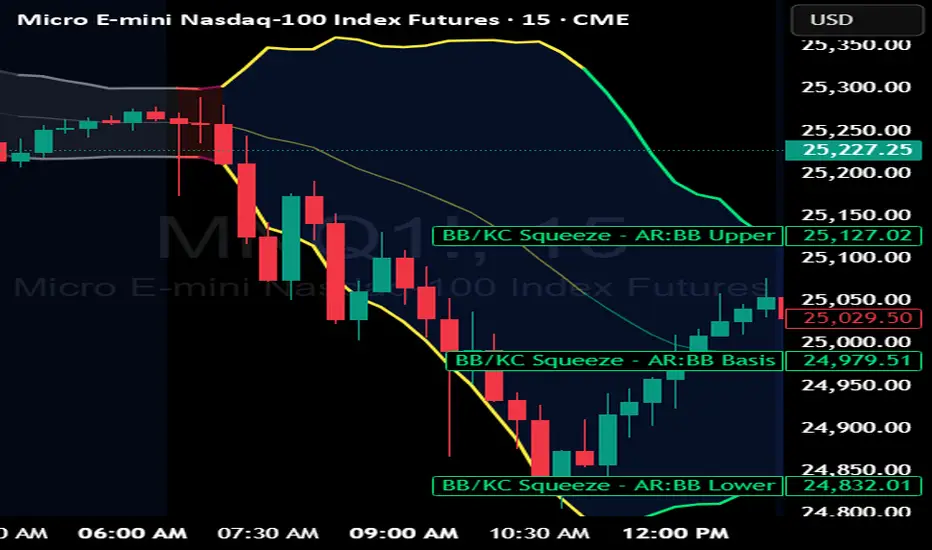
BB Keltner Squeeze - ArchReactorBollinger Band - Ketlner Squeeze .
Typical definition is when Bollinger band upper and lower is inside Ketlner channels , its when the squeeze happens.
Maybe helpful in developing strats around squeeze and the squeeze is displayed right on the chart.
Hurst Dual-Channel + ECDF Early Reentry (Single Trigger)Hello,
This indicator can be useful during ranging market phases, especially on short timeframes such as 5 minutes, within a statistically contrarian approach.
It combines two quantitative methodologies:
– Hurst-type adaptive channels, which measure short- and medium-term price deviations using the ATR (Average True Range);
– an Empirical Cumulative Distribution Function (ECDF), which locates the current price between its recent extremes (0 corresponding to the lower bound, 1 to the upper bound).
The goal is to identify relative overbought and oversold zones, where the price exceeds the channels and then begins to revert toward its statistical mean.
The indicator does not issue trading recommendations: it merely highlights specific statistical conditions for research and analytical purposes.
The “BUY” and “SELL” labels indicate such technical configurations:
– ECDF < 0.2 with price returning above the lower channels → bullish reentry.
– ECDF > 0.9 with price returning below the upper channels → bearish reentry.
The parameters (channel periods, ECDF window, smoothing) allow you to fine-tune the sensitivity of the analysis according to instrument volatility or chosen timeframe.
🟩 Buy Signal (BUY)
A buy signal is triggered when a strong downside deviation pushes the price below both channels, followed by a gradual reentry inside the bands.
More precisely:
– The low is below both channels (low < scb and low < mcb).
– The ECDF crosses back above 0.19 (exit from oversold).
– Both events occur within the last six bars.
– The price moves back above the lower channel (high > scb).
– No previous long signal is active.
This configuration represents a statistical reentry to the mean after an excessive drop.
🟥 Sell Signal (SELL)
Conversely, a sell signal appears when a strong upside deviation pushes the price above both channels, followed by a pullback below them:
– The high exceeds both channels (high > sct and high > mct).
– The ECDF crosses below 0.9 (exit from overbought).
– Both events occur within the last six bars.
– The price falls back below the upper channel (low < sct).
– No previous short signal is active.
This reflects a bearish reentry following a statistical overextension.
⚙️ Operating Logic
Each signal is triggered only once per cycle thanks to the variables triggered_long and triggered_short, preventing duplicates until a new extreme occurs.
The tool is designed for visual analysis and pattern research, not for automated execution.
🔍 ECDF Principle and Calculation
The ECDF is a non-parametric measure of a value’s position within its recent distribution:
ECDF(X)=number of values ≤XNECDF(X) = \frac{\text{number of values } \le X}{N}ECDF(X)=Nnumber of values ≤X
It expresses the empirical proportion of observations below the current value.
Example:
If, among the last 100 observations, 85 are below the current price, then
ECDF=0.85ECDF = 0.85ECDF=0.85
→ The price is at the 85th percentile, statistically high relative to recent history.
Strengths: robust, model-free, well-suited to asymmetric or non-normal market regimes.
Limitations: it does not measure amplitude and depends on the selected window size.
🌊 Intuitive Analogy: The River and the Gauge
Imagine a river with a depth gauge:
– The Z-Score tells you how many meters above the average level the water currently stands.
– The ECDF tells you in how many past cases the water level was lower than it is now.
The Z-Score assumes the river always follows the same symmetrical pattern.
The ECDF simply observes reality — adapting naturally, even when the current becomes unpredictable.
Final note:
This indicator is designed for visual and statistical exploration of price behavior.
The signals represent statistical states, not trade instructions.
Entering long or short positions based on them is entirely at your own discretion and risk.

Institutional Rolling VWAPs • 3 lines Institutional Rolling VWAPs • 3 lines + editable σ bands. 3 x modifiable vwaps, time anchored, same for ltf and htf

Plot_4_Key_LevelsBollinger Bands (upper & lower)
- computes 12-bar Bollinger Bands on the chart’s current timeframe, with a 3σ (standard-deviation) multiplier.
- computes vwap
- computes VWMA(HL2, 36)—a smoothed, volume-weighted average price—plotted as a line.

Master Simple Indicator 2.0Master Simple Indicator 2.0 combines dynamic moving average signals with ATR-based price bands. It plots a volatility range around the current price using customizable ATR length, smoothing, and multiplier settings, while also highlighting long/short opportunities when price crosses a 120-period moving average. Visual cues and alerts help identify momentum shifts, trend direction, and potential trade entries across all timeframes.

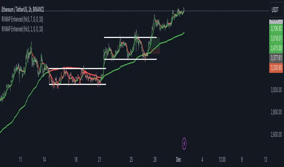
RVWAP ENHANCED**Rolling VWAP with Alerts and Markers**
This Pine Script indicator enhances the traditional Rolling VWAP (Relative Volume Weighted Average Price) by adding dynamic features for improved visualization and alerting.
### Features:
1. **Dynamic VWAP Line Coloring**:
- The VWAP line changes color based on the relationship with the closing price:
- **Green** when the price is above the VWAP.
- **Red** when the price is below the VWAP.
2. **Candle and Background Coloring**:
- **Candles**: Colored green if the close is above the VWAP and red if below.
- **Background**: Subtle green or red shading indicates the price’s position relative to the VWAP.
3. **Alerts**:
- Alerts notify users when the VWAP changes direction:
- "VWAP Turned Green" for price crossing above the VWAP.
- "VWAP Turned Red" for price crossing below the VWAP.
4. **Small Dot Markers**:
- Tiny dots are plotted below the candles to mark VWAP state changes:
- **Green dot** for VWAP turning green.
- **Red dot** for VWAP turning red.
5. **Custom Time Period**:
- Users can select either a dynamic time period based on the chart's timeframe or a fixed time period (customizable in days, hours, and minutes).
6. **Standard Deviation Bands (Optional)**:
- Standard deviation bands around the VWAP can be enabled for further analysis.
This script is designed to provide clear and actionable insights into market trends using the RVWAP, making it an excellent tool for traders who rely on volume-based price action analysis.
Contrarian Donchian Channel Indicator with Alerts and VisualsTitle: Contrarian Donchian Channel Indicator with Alerts and Visuals
Description:
The Contrarian Donchian Channel Indicator is designed for traders who seek to implement a contrarian approach using the time-tested Donchian Channel method. This indicator not only signals potential entry points but also enhances trading visualization by marking hypothetical stop loss and take profit levels.
Key Features:
Donchian Channel Signals: Utilizes the Donchian Channel to identify potential reversal points in the market. The indicator generates buy signals when the price touches or breaches the lower band, suggesting a potential upward reversal. Conversely, sell signals are generated when the price touches or exceeds the upper band, indicating a possible downward reversal.
Pause After Stop Loss: Incorporates a unique feature that pauses signal generation for a user-defined number of candles after a stop loss is hit. This helps in avoiding immediate re-entries in volatile market conditions.
Stop Loss and Take Profit Visualization: For each signal, the indicator draws dashed lines on the chart to represent the hypothetical stop loss (red) and take profit (green) levels. These levels are calculated based on user-input percentages for stop loss and the risk-reward ratio.
Alerts for Entry Signals: Traders can set up alerts for buy and sell signals, allowing them to stay informed of potential trading opportunities.
How to Use:
Entry Signal: A triangle symbol (green for buy, red for sell) accompanied by an alert (if set) indicates a potential entry point.
Stop Loss and Take Profit Lines: Use the drawn lines as a guide for setting stop loss and take profit levels if the signal aligns with your trading strategy.
Pause Feature: After a stop loss is triggered, observe the pause period before considering new signals to avoid overtrading in choppy markets.
Suitable For:
Traders who prefer a contrarian approach.
Those who use Donchian Channels as part of their trading strategy.
Traders who appreciate visual aids for better decision-making.
Customization Options:
Length of the Donchian Channel.
Risk/Reward Ratio.
Stop Loss Percentage.
Pause duration after a stop loss is hit.
DISCLAIMER:
This indicator is intended for educational and informational purposes only and should not be construed as financial advice. Trade responsibly and always consider your risk tolerance and investment objectives.

Moving Average SARHello Traders,
Today, I have brought to you an indicator that utilizes the Parabolic SAR.
To begin with, the Parabolic SAR is an indicator that trails the price in the form of a parabola, seeking out Stop And Reverse points.
The indicator I present merges the calculation formula of the Parabolic SAR with the Moving Average.
One aspect I pondered over was how to determine the starting point of this SAR. Trailing the price flow with the logic set by the moving average was fine, but the question was where to begin.
My approach involves a variable I call 'sensitiveness,' which automatically adjusts the length according to the timeframe you are observing. Using pinescript's math.ceil, I formulated:
interval_to_len = timeframe.multiplier * (timeframe.isdaily ? 1440 : timeframe.isweekly ? 1440 * 7 : timeframe.ismonthly ? 1440 * 30 : 1)
main_len = math.ceil(sensitiveness / interval_to_len)
This formula represents the length, and through variables like:
_highest = math.min(ta.highest(high, main_len), close + ta.atr(46)*4)
_lowest = math.max(ta.lowest(low, main_len), close - ta.atr(46)*4)
I have managed to set the risk at a level that does not impose too great a burden.
Moreover, the 'Trend Strength Parameter' allows you to choose how strongly to trail the current price.
Lastly, think of the Band Width as a margin for accepting changes in the trend. As the value increases, the Band Width expands, measured through the ATR.
This indicator is particularly useful for holding positions and implementing trailing stops. It will be especially beneficial for those interested in price tracking of trends, like with Parabolic SAR or Supertrend.
I hope you find this tool useful.

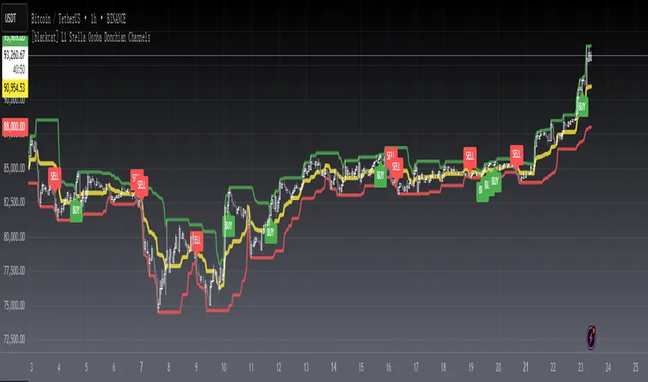
[blackcat] L1 Stella Osoba Donchian ChannelsLevel 1
Background
On Jul, 2023, Stella Osoba proposed a price channel idea in the article of “Using Price Channels”.
Function
In Stella Osoba's article "Using Price Channels" in the 2023 bonus issue, author Stella Osoba describes why many analysis techniques are based on the concept of price channels. In her explanation of the Donchian channels, she explains that they are used to identify the trend and that the prices for the last period are not included in the calculations. I rewrote this idea in the PINE version presented here, allowing the user to optionally include the most recent period. To not include the most recent period, set the IncludeRecentPeriod input to false.
Richard Donchian, a futures trader, created the Donchian Channel as a trend indicator. He was later dubbed the "father of trend following." Several trading methods based on Donchian channels have been established, but day traders can create their own as the indicator is versatile and can be interpreted in different ways. The renowned Turtle Traders also used a variation of the Donchian technique.
The Donchian Channel draws a line between the high and low price of an asset over a period of time, generally using candlesticks as a clock. Candlesticks are chart areas on charts that show the open, high, low, and close price and time frame of a particular stock. They owe their name to their shape. When the indicator is applied to a chart, the lines form a channel around the current price.
When day trading, Donchian channels are useful for highlighting trends and range periods. A third line can be added between the top and bottom lines if required. The upper and lower channel lines are averaged to form this center band. The indicator can be used on all timeframes, including one-minute and five-minute charts (where a bar forms every one or five minutes), and it can be used for forex, stock, futures, and options trading .
Remarks
Feedbacks are appreciated.
actic-fibbA fibbonacci based bollinger band. Up and down trading arrows are generated based on crossover and crossunder of 200 day vma

RSI by JBTRelative Strength Index With Alerts. With an upper band of crossing over 62 (RSI) and a lower band with a Triger price of 32 (RSI), This saves time and effort in waiting for the price to move above the desired level.
Hitokiri rsi and bbNG : This indicator is created by combining the standard period RSI indicator with an Oversold limit of 32, an Overbought limit of 70 and a period of 14 (these values can be changed optionally from the entries and still tabs of the indicator settings) and the Bollinger Band . indicator with a standard deviation of 2 and a period of 20. Also, the RSI Oversold is an upward green triangle where the price simultaneously falls below the BB and the lower limit (Low) (i.e. below 32), where the RSI Overbought (i.e. above 70) at the same time the price rises above the BB and the upper limit (Upper) is a downward red triangle. is indicated by a triangle. An alarm condition is established on these conditions. Source codes are posted visually and written in clear language and with explanations for beginners to learn to pine.
TR : Bu gösterge OverSold sınırı 32, OverBought sınırı 70 ve periodu 14 olan (bu değerler tercihe göre indikatör ayarlarının girdiler ve still sekmelerinden değiştirilebilir) standart periodluk RSI göstergesi ile standart sapma değeri 2, periodu 20 olan Bollinger Bandı göstergesinin birleştirilmesiyle oluşturulmuş olup ilaveten RSI'nin OverSold iken (yani 32 altına düştüğü) aynı anda fiyatın BBand alt sınırı (Lower) altına düştüğü yerleri yukarı yönlü yeşil üçgenle, RSI'nin OverBought iken (yani 70 üstüne çıktığı) aynı anda fiyatın BBand üst sınırı (Upper) üstüne çıktığı yerleri aşağı yönlü kırmızı üçgenle belirtmektedir. Bu şartlar üzerine de alarm kondüsyonu oluşturulmuştur. Kaynak kodları görünür olarak yayınlanmış olup, pine öğrenmeye yeni başlayanlar için anlaşılır dilde ve açıklamalar eklenerek yazılmıştır.

Happy KCRe-interpreted from @eSaniello for visual purposes and re-worked the math on the Keltner formula.
Keltner Channel Calculation
Keltner Channel Middle Line=EMA
Keltner Channel Upper Band=EMA+multiplier∗ATR
Keltner Channel Lower Band=EMA−multiplier∗ATR
where:
EMA=Exponential moving average (typically over 20 periods)
ATR=Average True Range (typically over 10 or 20 periods)
I wanted dual Keltner channels in a single indicator. If you add the default Tradingview Keltner channels twice with multipliers of 1 and 2, it should overlay exactly.

HURST Channel StrategyBased on the work TJS / Trading Zoom / Svoboda
Strategy based on Hurst channel with loss averaging when an open position is below 0.5 channel range.
How it works:
1. opens the long position when the close price crosses over the lower band (from bottom to top)
2. opens additional position (double in size) when average position price is lower than average channel value (0.5)
3. closes the position when the close price crosses over the higher band (from top to bottom)
Works the best on :
- volatile and continuous instruments (futures)
- on timeframes above 15 minutes
- uptrends or consolidations
- downtrends require more capital to open double positions
