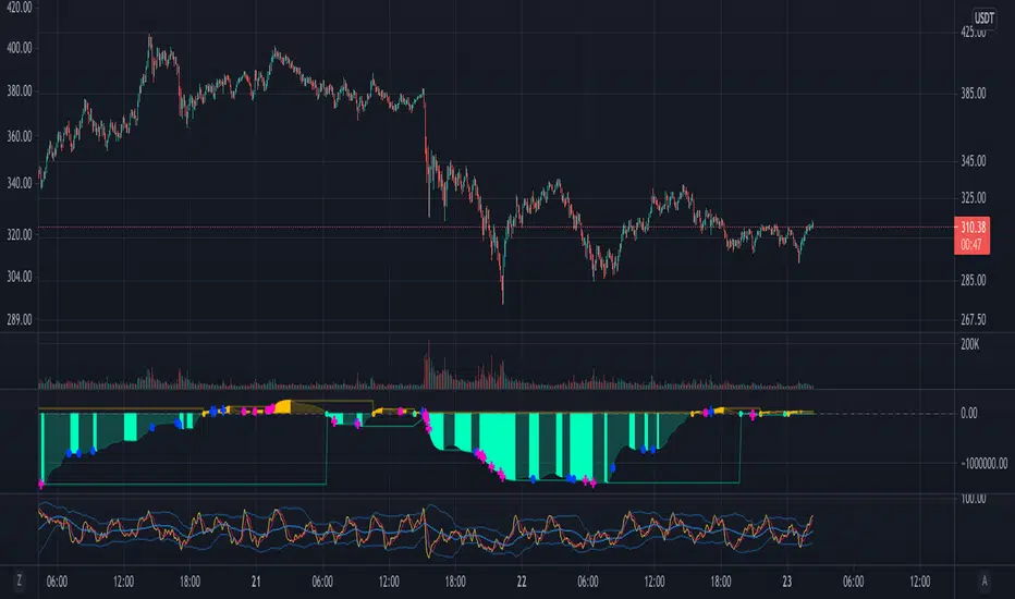
Market Maker BalanceWhere is the market maker in his cycle of building longs or shorts? When is that big drop or big pump coming?
This is a simple and unexpectedly powerful indicator that shows you an estimate of the market maker's position over the last 200 candles. It works on any timeframe.
How does it work?
It combines a simple 10-candle Price Volume Support Resistance Analysis metric of climactic and rising volume. That volume is combined to create a bullish and bearish balance over a period of 200 candles. The curves are smoothed out with a 10 period EMA.
The MMB (Marker Maker Balance) oscillator is the resulting bearish volume - bullish volume, which shows us THEIR position balance.
Indications:
when shorts are increasing (further below 0), we are in a bullish trend -- you should be taking profit on longs
when shorts are flat or decreasing, the trend is due for a reversal -- you should be closing longs and looking to short
when shorts cross 0 to long, the trend is reversing down -- you should be in a short position by now
when longs are increasing, we are in a bearish trend -- you should be taking profits on your shorts
when longs are flat or decreasing, the trend is due for a reversal -- you should be closing your shorts
For extra information, there are also the separate lines for rising and climactic volume to give you early indications of reversal or change in Market Maker behaviour. You can disable them in the Style settings, but they can be a useful early indicator that the current trend is losing strength when rising volume overtakes climax volume (MM's no longer moving out of zones higher/lower).
Ways to use this indicator are quite simple and eerily accurate:
for short term gains, do the opposite of MMs: long when MM are opening more shorts, short when they are opening more longs
for huge positions, mimic the MM position: build long positions / close shorts when MMB is rising, build shorts / close longs when MMB is falling or crosses above 0 (be careful with leverage, begin on 1x leverage)
Note: the results of this indicator will be different for each exchange, because of their different trading volumes per candle. It's advisable to use it for the exchange you're trading on or use a chart that averages all exchanges for that asset, like INDEX:BTCUSD.
For those of you who use the Backtesting & Trading Engine by PineCoders, the BTE Signal plot generates long and short entries as well as filter states. Use this plot as the source for BTE.
Shout out to @infernixx for PVSRA calculations in his awesome Traders Reality indicator, the code of which I shamelessly ripped off and edited for this indicator.
Leave comments below if you want something added.
Search in scripts for "curve"
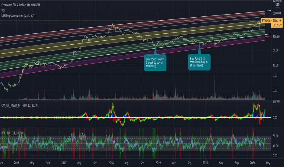
Ethereum Logarithmic Growth Curves & ZonesThis script was modified to fit ethereum logarithmic pricing action.
Moving Regression Prediction BandsIntroducing the Moving Regression Prediction Bands indicator.
Here I aimed to combine the principles of traditional band indicators (such as Bollinger Bands), regression channel and outlier detection methods. Its upper and lower bands define an interval in which the current price was expected to fall with a prescribed probability, as predicted by the previous-step result of the local polynomial regression (for the original Moving Regression script, see link below).
Algorithm
1. At every time step, the script performs local polynomial regression of the sample data within the lookback window specified by the Length input parameter.
2. The fitted polynomial is used to construct the Moving Regression time series as well as to extrapolate data, that is, to predict the next data point ( MRPrediction ).
3. The accuracy of local interpolation is estimated by means of the root-mean-square error ( RMSE ), that is, the deviation between the fitted polynomial and the observed values.
4. The MRPrediction and RMSE values calculated for the previous bar are then used to build the upper and lower bands , which I define as follows:
Upper Band = MRPrediction_prev + Multiplier *( RMSE_prev )
Lower Band = MRPrediction_prev - Multiplier *( RMSE_prev )
Here the Multiplier is a user-defined parameter that should be interpreted as a quantile in the standard normal distribution (the default value of 2.0 roughly corresponds to the 95% prediction interval).
To visualize the central line , the script offers the following options:
Previous-Period MR Prediction: MRPrediction_prev time series from the above equation.
MR: Conventional Moving Regression time series.
Ribbon: “Previous-Period MR Prediction” and “MR” curves plotted together and colored according to their relative value (green if MR > Previous MR Prediction; red otherwise).
Usage
My original idea was to use the band breakouts as potential trading signals. For example, the price crossing above the upper band is a bullish signal , being a potential sign that price is gaining momentum and is out of a previously predicted trend. The exit signal could be the crossing under the lower band or under the central line.
However, be aware that it is an experimental indicator, so you might fin some better strategies.
Feel free to play around!

Trend ChannelMarket engineers can use channels to find out when a market has entered an undervalued or overvalued zone. Purchases and sales take place in these zones. Professionals use trending channels to find out when the market has overtaken itself and where it is likely to reverse.
Upper channel line = EMA + EMA x channel coefficient
Lower channel line = EMA - EMA x channel coefficient
The topline reflects the bulls' strength in raising prices above the average value consensus. This line marks the normal limit of optimism in the market.
The bottom line of the channel reflects the strength of the bears pushing prices below the average consensus of values. This line marks the normal limit of pessimism in the market.
The coefficient is used to correct the distance to the moving average until the channel contains 95% of all prices. Only the tips and the lowest bottoms are allowed to protrude. For these peaks and curves and sideways trends, I have added two more switchable lines to the border lines, with a distance of 23.6% (light blue).
The larger the time frame, the wider the channel.
If you buy near a rising moving average, you take profits near the upper line of the channel.
If you are short near a falling moving average, you should close out near the bottom of the channel.
If the moving average is essentially flat, then you should be long on the bottom of the channel and short on the top of the channel. You realize profits when the prices have returned to their moving average to normal.
Interesting for day traders:
Adjust the moving average so that it has the same slope as the quotes on the hourly chart. With the coefficient you set the distance between the border lines. Perhaps adding the 23.6% lines will help, where the sideways trends are starting. Set the resolution to "1 hour". If you want to trade with these settings in short time units, e.g. in the 3 minute chart or in the 1 minute chart, then you now have target marks and indications in which direction the prices will possibly move when the prices have reached the moving average or one of the border lines.
The text contains excerpts from "Come into my Trading Room" by Dr. Alexander Elder.
The indicator has an additional exponential moving average with adjustable period, adjustable shift and adjustable source for the narrow range of quotations and final determination of direction.
The chart shows how the trend channel and the Fibonacc trading indicator can complement each other.
The text contains excerpts from "Come into my Trading Room" by Dr. Alexander Elder.
Markttechniker können Kanäle verwenden um heraus zu finden, wann ein Markt eine unterbewertete oder überbewertete Zone erreicht hat. An diesen Zonen finden Käufe und Verkäufe statt. Profis benutzen Trendkanäle um herauszufinden, wann der Markt sich selbst überholt hat und wo er wahrscheinlich eine Umkehrbewegung vollziehen wird.
Obere Kanallinie = EMA + EMA x Kanalkoeffizient
Untere Kanallinie = EMA - EMA x Kanalkoeffizient
Die Oberlinie reflektiert die Kraft der Bullen, mit der sie die Kurse über den durchschnittlichen Wertekonsens anheben. Diese Linie kennzeichnet die normale Grenze des Optimismus im Markt.
Die untere Linie des Kanals reflektiert die Kraft der Bären, mit der sie die Kurse unter den durchschnittlichen Wertekonsens drücken. Diese Linie kennzeichnet die normale Grenze des Pessimismus im Markt.
Mit dem Koeffizienten wird der Abstand zum gleitenden Durchschnitt so lange korrigiert, bis der Kanal 95% aller Kurse enthält. Lediglich die Spitzen und die niedrigsten Böden dürfen herausragen. Für diese Spitzen und Bögen und Seitwärtstrends habe ich zu den Grenzlinien zwei weitere zuschaltbare Linien, mit einem Abstand von 23,6%, hinzugefügt (hellblau).
Je größer der Zeitrahmen ist, um so breiter ist der Kanal.
Wenn Sie in der Nähe eines ansteigenden gleitenden Durchschnitts kaufen, nehmen Sie die Gewinne in der Nähe der oberen Grenzlinie des Kanals mit.
Wenn Sie in der Nähe eines fallenden gleitenden Durchschnitts leerverkaufen, sollten Sie in der Nähe der unteren Grenzlinie des Kanals glattstellen.
Wenn der gleitende Durchschnitt im Wesentlichen flach ist, dann sollten Sie an der unteren Kanalbegrenzung eine Long-Position und an der oberen Kanalbegrenzung eine Short-Position einnehmen. Gewinne realisieren Sie jeweils, wenn die Kurse zu ihrem gleitenden Durchschnitt, zur Normalität zurückgekehrt sind.
Für Daytrader interessant:
Stellen Sie den gleitenden Durchschnitt so ein, dass er die gleiche Steigung wie die Notierungen im Stunden-Chart hat. Mit dem Koeffizienten Stellen Sie den Abstand der Grenzlinien ein. Vielleicht hilft die Zuschaltung der 23,6%-Linien, wo die Seitwärtstrends anstoßen. Stellen Sie die Auflösung auf „1 Stunde“. Wenn Sie mit diesen Einstellungen in niedrigen Zeiteinheiten traden wollen, z.B. im 3 Minuten-Chart oder im 1 Minuten-Chart, dann haben Sie jetzt Zielmarken und Hinweise in welche Richtung die Notierungen möglicherweise laufen werden, wenn die Notierungen den gleitenden Durchschnitt oder eine der Grenzlinien erreicht haben.
Der Text enthält Auszüge aus „Come into my Trading Room“ von Dr. Alexander Elder.
Der Indikator besitzt zur engen Umfang der Notierungen und endgültigen Richtungsbestimmung einen zusätzlichen exponentiellen gleitenden Durchschnitt mit einstellbarer Periode, einstellbarer Verschiebung und einstellbarer Quelle.
Der Chart zeigt wie sich Trendkanal und Fibonacc-Trading-Indikator ergänzen könne.
Der Text enthält Auszüge aus „Come into my Trading Room“ von Dr . Alexander Elder.

Square Root Moving AverageAbstract
This script computes moving averages which the weighting of the recent quarter takes up about a half weight.
This script also provides their upper bands and lower bands.
You can apply moving average or band strategies with this script.
Introduction
Moving average is a popular indicator which can eliminate market noise and observe trend.
There are several moving average related strategies used by many traders.
The first one is trade when the price is far from moving average.
To measure if the price is far from moving average, traders may need a lower band and an upper band.
Bollinger bands use standard derivation and Keltner channels use average true range.
In up trend, moving average and lower band can be support.
In ranging market, lower band can be support and upper band can be resistance.
In down trend, moving average and upper band can be resistance.
An another group of moving average strategy is comparing short term moving average and long term moving average.
Moving average cross, Awesome oscillators and MACD belong to this group.
The period and weightings of moving averages are also topics.
Period, as known as length, means how many days are computed by moving averages.
Weighting means how much weight the price of a day takes up in moving averages.
For simple moving averages, the weightings of each day are equal.
For most of non-simple moving averages, the weightings of more recent days are higher than the weightings of less recent days.
Many trading courses say the concept of trading strategies is more important than the settings of moving averages.
However, we can observe some characteristics of price movement to design the weightings of moving averages and make them more meaningful.
In this research, we use the observation that when there are no significant events, when the time frame becomes 4 times, the average true range becomes about 2 times.
For example, the average true range in 4-hour chart is about 2 times of the average true range in 1-hour chart; the average true range in 1-hour chart is about 2 times of the average true range in 15-minute chart.
Therefore, the goal of design is making the weighting of the most recent quarter is close to the weighting of the rest recent three quarters.
For example, for the 24-day moving average, the weighting of the most recent 6 days is close to the weighting of the rest 18 days.
Computing the weighting
The formula of moving average is
sum ( price of day n * weighting of day n ) / sum ( weighting of day n )
Day 1 is the most recent day and day k+1 is the day before day k.
For more convenient explanation, we don't expect sum ( weighting of day n ) is equal to 1.
To make the weighting of the most recent quarter is close to the weighting of the rest recent three quarters, we have
sum ( weighting of day 4n ) = 2 * sum ( weighting of day n )
If when weighting of day 1 is 1, we have
sum ( weighting of day n ) = sqrt ( n )
weighting of day n = sqrt ( n ) - sqrt ( n-1 )
weighting of day 2 ≒ 1.414 - 1.000 = 0.414
weighting of day 3 ≒ 1.732 - 1.414 = 0.318
weighting of day 4 ≒ 2.000 - 1.732 = 0.268
If we follow this formula, the weighting of day 1 is too strong and the moving average may be not stable.
To reduce the weighting of day 1 and keep the spirit of the formula, we can add a parameter (we call it as x_1w2b).
The formula becomes
weighting of day n = sqrt ( n+x_1w2b ) - sqrt ( n-1+x_1w2b )
if x_1w2b is 0.25, then we have
weighting of day 1 = sqrt(1.25) - sqrt(0.25) ≒ 1.1 - 0.5 = 0.6
weighting of day 2 = sqrt(2.25) - sqrt(1.25) ≒ 1.5 - 1.1 = 0.4
weighting of day 3 = sqrt(3.25) - sqrt(2.25) ≒ 1.8 - 1.5 = 0.3
weighting of day 4 = sqrt(4.25) - sqrt(3.25) ≒ 2.06 - 1.8 = 0.26
weighting of day 5 = sqrt(5.25) - sqrt(4.25) ≒ 2.3 - 2.06 = 0.24
weighting of day 6 = sqrt(6.25) - sqrt(5.25) ≒ 2.5 - 2.3 = 0.2
weighting of day 7 = sqrt(7.25) - sqrt(6.25) ≒ 2.7 - 2.5 = 0.2
What you see and can adjust in this script
This script plots three moving averages described above.
The short term one is default magenta, 6 days and 1 atr.
The middle term one is default yellow, 24 days and 2 atr.
The long term one is default green, 96 days and 4 atr.
I arrange the short term 6 days to make it close to sma(5).
The other twos are arranged according to 4x length and 2x atr.
There are 9 curves plotted by this script. I made the lower bands and the upper bands less clear than moving averages so it is less possible misrecognizing lower or upper bands as moving averages.
x_src : how to compute the reference price of a day, using 1 to 4 of open, high, low and close.
len : how many days are computed by moving averages
atr : how many days are computed by average true range
multi : the distance from the moving average to the lower band and the distance from the moving average to the lower band are equal to multi * average true range.
x_1w2b : adjust this number to avoid the weighting of day 1 from being too strong.
Conclusion
There are moving averages which the weighting of the most recent quarter is close to the weighting of the rest recent three quarters.
We can apply strategies based on moving averages. Like most of indicators, oversold does not always means it is an opportunity to buy.
If the short term lower band is close to the middle term moving average or the middle term lower band is close to the long term moving average, it may be potential support value.
References
Computing FIR Filters Using Arrays
How to trade with moving averages : the eight trading signals concluded by Granville
How to trade with Bollinger bands
How to trade with double Bollinger bands
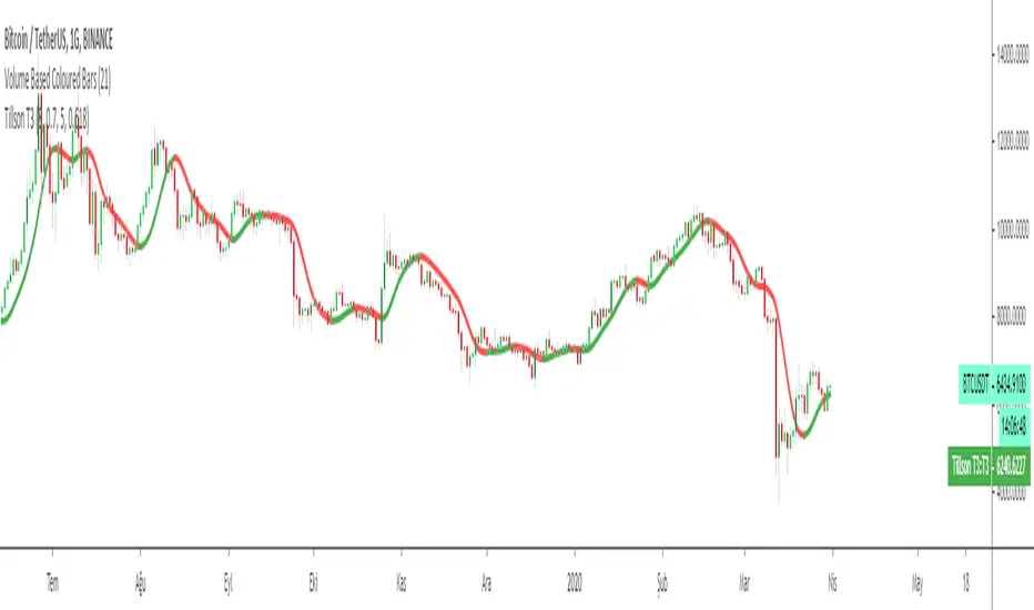
Tilson T3 and MavilimW Triple Combined StrategyInspired by truly greatful Kivanç Ozbilgic (www.tradingview.com).
The strategy tries to combined three different moving average strategies into one.
Strategies covered are:
1. Tillson T3 Moving Average Strategy
Developed by Tim Tillson, the T3 Moving Average is considered superior to traditional moving averages as it is smoother, more responsive and thus performs better in ranging market conditions as well. However, it bears the disadvantage of overshooting the price as it attempts to realign itself to current market conditions.
It incorporates a smoothing technique which allows it to plot curves more gradual than ordinary moving averages and with a smaller lag. Its smoothness is derived from the fact that it is a weighted sum of a single EMA, double EMA, triple EMA and so on. When a trend is formed, the price action will stay above or below the trend during most of its progression and will hardly be touched by any swings. Thus, a confirmed penetration of the T3 MA and the lack of a following reversal often indicates the end of a trend. Here is what the calculation looks like:
T3 = c1*e6 + c2*e5 + c3*e4 + c4*e3, where:
– e1 = EMA (Close, Period)
– e2 = EMA (e1, Period)
– e3 = EMA (e2, Period)
– e4 = EMA (e3, Period)
– e5 = EMA (e4, Period)
– e6 = EMA (e5, Period)
– a is the volume factor, default value is 0.7 but 0.618 can also be used
– c1 = – a^3
– c2 = 3*a^2 + 3*a^3
– c3 = – 6*a^2 – 3*a – 3*a^3
– c4 = 1 + 3*a + a^3 + 3*a^2
T3 MovingThe T3 Moving Average generally produces entry signals similar to other moving averages and thus is traded largely in the same manner.
Strategy for Tillson T3 is if the close crossovers T3 line and for at least five bars the close was under the T3
2. Tillson T3 Fibonacci Cross
Kivanc Ozbilgic added a second T3 line with a volume factor of 0.618 (Fibonacci Ratio) and length of 3 (fibonacci number) which can be added by selecting the T3 Fibonacci Strategy input box.
Strategy for Tillson T3 Fibo is when the Fibo Line crossover the T3 it gives long signal vice versa.
3. MavilimW
MavilimW is originally a support and resistance indicator based on fibonacci injected weighted moving averages.
Strategy for MavilimW is is if the close crossovers T3 line and for at least five bars the close was under the T3
Hope you enjoy

[2020 Updated]Bitcoin Logarithmic Growth CurvesCredit goes to the original writer of the script, Quantadelic, who generously allowed anyone to copy/edit. I adjusted the value of the bottom/top intercept and slope to better fit the March 2020 coronavirus dip.
Use Bitstamp BTCUSD for better reading.

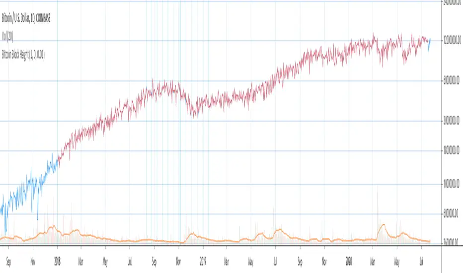
Bitcoin Block Height (Total Blocks)Bitcoin Block Height by RagingRocketBull 2020
Version 1.0
Differences between versions are listed below:
ver 1.0: compare QUANDL Difficulty vs Blockchain Difficulty sources, get total error estimate
ver 2.0: compare QUANDL Hash Rate vs Blockchain Hash Rate sources, get total error estimate
ver 3.0: Total Blocks estimate using different methods
--------------------------------
This indicator estimates Bitcoin Block Height (Total Blocks) using Difficulty and Hash Rate in the most accurate way possible, since
QUANDL doesn't provide a direct source for Bitcoin Block Height (neither QUANDL:BCHAIN, nor QUANDL:BITCOINWATCH/MINING).
Bitcoin Block Height can be used in other calculations, for instance, to estimate the next date of Bitcoin Halving.
Using this indicator I demonstrate:
- that QUANDL data is not accurate and differ from Blockchain source data (industry standard), but still can be used in calculations
- how to plot a series of data points from an external csv source and compare it with another source
- how to accurately estimate Bitcoin Block Height
Features:
- compare QUANDL Difficulty source (EOD, D1) with external Blockchain Difficulty csv source (EOD, D1, embedded)
- show/hide Quandl/Blockchain Difficulty curves
- show/hide Blockchain Difficulty candles
- show/hide differences (aqua vertical lines)
- show/hide time gaps (green vertical lines)
- count source differences within data range only or for the whole history
- multiply both sources by alpha to match before comparing
- floor/round both matched sources when comparing
- Blockchain Difficulty offset to align sequences, bars > 0
- count time gaps and missing bars (as result of time gaps)
WARNING:
- This indicator hits the max 1000 vars limit, adding more plots/vars/data points is not possible
- Both QUANDL/Blockchain provide daily EOD data and must be plotted on a daily D1 chart otherwise results will be incorrect
- current chart must not have any time gaps inside the range (time gaps outside the range don't affect the calculation). Time gaps check is provided.
Otherwise hardcoded Blockchain series will be shifted forward on gaps and the whole sequence become truncated at the end => data comparison/total blocks estimate will be incorrect
Examples of valid charts that can run this indicator: COINBASE:BTCUSD,D1 (has 8 time gaps, 34 missing bars outside the range), QUANDL:BCHAIN/DIFF,D1 (has no gaps)
Usage:
- Description of output plot values from left to right:
- c_shifted - 4x blockchain plotcandles ohlc, green/black (default na)
- diff - QUANDL Difficulty
- c_shifted - Blockchain Difficulty with offset
- QUANDL Difficulty multiplied by alpha and rounded
- Blockchain Difficulty multiplied by alpha and rounded
- is_different, bool - cur bar's source values are different (1) or not (0)
- count, number of differences
- bars, total number of bars/data points in the range
- QUANDL daily blocks
- Blockchain daily blocks
- QUANDL total blocks
- Blockchain total blocks
- total_error - difference between total_blocks estimated using both sources as of cur bar, blocks
- number_of_gaps - number of time gaps on a chart
- missing_bars - number of missing bars as result of time gaps on a chart
- Color coding:
- Blue - QUANDL data
- Red - Blockchain data
- Black - Is Different
- Aqua - number of differences
- Green - number of time gaps
- by default the indicator will show lots of vertical aqua lines, 138 differences, 928 bars, total error -370 blocks
- to compare the best match of the 2 sources shift Blockchain source 1 bar into the future by setting Blockchain Difficulty offset = 1, leave alpha = 0.01 =>
this results in no vertical aqua lines, 0 differences, total_error = 0 blocks
if you move the mouse inside the range some bars will show total_error = 1 blocks => total_error <= 1 blocks
- now uncheck Round Difficulty Values flag => some filled aqua areas, 218 differences.
- now set alpha = 1 (use raw source values) instead of 0.01 => lots of filled aqua areas, 871 differences.
although there are many differences this still doesn't affect the total_blocks estimate provided Difficulty offset = 1
Methodology:
To estimate Bitcoin Block Height we need 3 steps, each step has its own version:
- Step 1: Compare QUANDL Difficulty vs Blockchain Difficulty sources and estimate error based on differences
- Step 2: Compare QUANDL Hash Rate vs Blockchain Hash Rate sources and estimate error based on differences
- Step 3: Estimate Bitcoin Block Height (Total Blocks) using different methods in the most accurate way possible
QUANDL doesn't provide block time data, but we can calculate it using the Hash Rate approximation formula:
estimated Hash rate/sec H = 2^32 * D / T, where D - Difficulty, T - block time, sec
1. block time (T) can be derived from the formula, since we already know Difficulty (D) and Hash Rate (H) from QUANDL
2. using block time (T) we can estimate daily blocks as daily time / block time
3. block height (total blocks) = cumulative sum of daily blocks of all bars on the chart (that's why having no gaps is important)
Notes:
- This code uses Pinescript v3 compatibility framework
- hash rate is in THash/s, although QUANDL falsely states in description GHash/s! THash = 1000 GHash
- you can't read files, can only embed/hardcode raw data in script
- both QUANDL and Blockchain sources have no gaps
- QUANDL and Blockchain series are different in the following ways:
- all QUANDL data is already shifted 1 bar into the future, i.e. prev day's value is shown as cur day's value => Blockchain data must be shifted 1 bar forward to match
- all QUANDL diff data > 1 bn (10^12) are truncated and have last 1-2 digits as zeros, unlike Blockchain data => must multiply both values by 0.01 and floor/round the results
- QUANDL sometimes rounds, other times truncates those 1-2 last zero digits to get the 3rd last digit => must use both floor/round
- you can only shift sequences forward into the future (right), not back into the past (left) using positive offset => only Blockchain source can be shifted
- since total_blocks is already a cumulative sum of all prev values on each bar, total_error must be simple delta, can't be also int(cum()) or incremental
- all Blockchain values and total_error are na outside the range - move you mouse cursor on the last bar/inside the range to see them
TLDR, ver 1.0 Conclusion:
QUANDL/Blockchain Difficulty source differences don't affect total blocks estimate, total error <= 1 block with avg 150 blocks/day is negligible
Both QUANDL/Blockchain Difficulty sources are equally valid and can be used in calculations. QUANDL is a relatively good stand in for Blockchain industry standard data.
Links:
QUANDL difficulty source: www.quandl.com
QUANDL hash rate source: www.quandl.com
Blockchain difficulty source (export data as csv): www.blockchain.com
Dual_Spread_FTX[Schmittie]//This script displays 2 spreads between FTX perpetuals contracts and futures contracts.
//In the settings, you can choose which curves to display for direct comparison.
//It is based on Thojdid's Multi-Spread script, but loads faster as there are only 2 coins
//An high-low range can be added

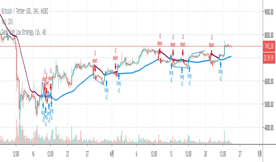
Gann High Low StrategyGann High Low is a moving average based trend indicator consisting of two different simple moving averages.
The Gann High Low Activator Indicator was described by Robert Krausz in a 1998 issue of Stocks & Commodities Magazine. It is a simple moving average SMA of the previous n period's highs or lows.
The indicator tracks both curves (of the highs and the lows). The close of the bar defines which of the two gets plotted.
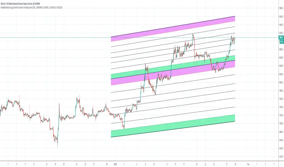
Bitcoin Logarithmic Growth Curves for intraday usersI wish to thank @Quantadelic who created this great indicator and leaving it open for others to improve.
I have made changes to make it user-friendly for the intraday traders.
The changes made have been;
1. Compartmentalized each area of the major Fibonacci level;
2. Added minor Fibonacci levels;
3. Color-coded the support and resistance levels, for better viewing;
4. Zoned each area of the major Fibonacci level; and
5. Created a time-frame display period for quicker loading of the indicator.
I have removed a few things to allow the indicator to run quicker;
1. Future projections; and
2. The major higher levels of the Fibonacci, which may be useful when Bitcoin reaches 100k.
Enjoy
Hull SuiteHull is its extremely responsive and smooth moving average created by Alan Hull in 2005.
Minimal lag and smooth curves made HMA extremely popular TA tool.
alanhull.com
Script was made to regroup multiple hull variants in one indicator,maintaining flexible customization and intuitive visualization
Option to chose between 3 Hull variations
Option to chose between 2 visualization modes ( Bands or single line)
Option to Paint hull and/or candlesticks according to hulls trend
Shortcut for personalizing Line/band thickness,instead of changing every object manually ,there is global option in inputs
HMA
THMA ( 3HMA)
EHMA
HMA:
Alan Hull
EHMA:
Slower than hull by default.
Raudys, Aistis & Lenčiauskas, Vaidotas & Malčius, Edmundas. (2013). Moving Averages for Financial Data Smoothing ( 403. 34-45. 10.1007/978-3-642-41947-8_4.) Vilnius University, Faculty of Mathematics and Informatics
3HMA (THMA) :
Documentation on link below
alexgrover

Gann High LowGann High Low is a moving average based trend indicator consisting of two different simple moving averages.
The Gann High Low Activator Indicator was described by Robert Krausz in a 1998 issue of Stocks & Commodities Magazine. It is a simple moving average SMA of the previous n period's highs or lows.
The indicator tracks both curves (of the highs and the lows). The close of the bar defines which of the two gets plotted.
This version is showing the channel that needs to be broken if the trend is going to be changed, and it allows you to chose from the 4 basic averages type for calculation (by definition, Gann High Low Activator uses only simple moving average, but some other averages can give you results that are probably more acceptable for trading in some conditions).
Increasing HPeriod and decreasing LPeriod better for short trades, vice versa for long positions.

Tillson T3 Moving Average MTFMULTIPLE TIME FRAME version of Tillson T3 Moving Average Indicator
Developed by Tim Tillson, the T3 Moving Average is considered superior -1.60% to traditional moving averages as it is smoother, more responsive and thus performs better in ranging market conditions as well. However, it bears the disadvantage of overshooting the price as it attempts to realign itself to current market conditions.
It incorporates a smoothing technique which allows it to plot curves more gradual than ordinary moving averages and with a smaller lag. Its smoothness is derived from the fact that it is a weighted sum of a single EMA , double EMA , triple EMA and so on. When a trend is formed, the price action will stay above or below the trend during most of its progression and will hardly be touched by any swings. Thus, a confirmed penetration of the T3 MA and the lack of a following reversal often indicates the end of a trend.
The T3 Moving Average generally produces entry signals similar to other moving averages and thus is traded largely in the same manner. Here are several assumptions:
If the price action is above the T3 Moving Average and the indicator is headed upward, then we have a bullish trend and should only enter long trades (advisable for novice/intermediate traders). If the price is below the T3 Moving Average and it is edging lower, then we have a bearish trend and should limit entries to short. Below you can see it visualized in a trading platform.
Although the T3 MA is considered as one of the best swing following indicators that can be used on all time frames and in any market, it is still not advisable for novice/intermediate traders to increase their risk level and enter the market during trading ranges (especially tight ones). Thus, for the purposes of this article we will limit our entry signals only to such in trending conditions.
Once the market is displaying trending behavior, we can place with-trend entry orders as soon as the price pulls back to the moving average (undershooting or overshooting it will also work). As we know, moving averages are strong resistance/support levels, thus the price is more likely to rebound from them and resume its with-trend direction instead of penetrating it and reversing the trend.
And so, in a bull trend, if the market pulls back to the moving average, we can fairly safely assume that it will bounce off the T3 MA and resume upward momentum, thus we can go long. The same logic is in force during a bearish trend .
And last but not least, the T3 Moving Average can be used to generate entry signals upon crossing with another T3 MA with a longer trackback period (just like any other moving average crossover). When the fast T3 crosses the slower one from below and edges higher, this is called a Golden Cross and produces a bullish entry signal. When the faster T3 crosses the slower one from above and declines further, the scenario is called a Death Cross and signifies bearish conditions.
I Personally added a second T3 line with a volume factor of 0.618 (Fibonacci Ratio) and length of 3 (fibonacci number) which can be added by selecting the box in the input section. traders can combine the two lines to have Buy/Sell signals from the crosses.
Developed by Tim Tillson

Tillson T3 Moving Average by KIVANÇ fr3762Developed by Tim Tillson, the T3 Moving Average is considered superior to traditional moving averages as it is smoother, more responsive and thus performs better in ranging market conditions as well. However, it bears the disadvantage of overshooting the price as it attempts to realign itself to current market conditions.
It incorporates a smoothing technique which allows it to plot curves more gradual than ordinary moving averages and with a smaller lag. Its smoothness is derived from the fact that it is a weighted sum of a single EMA , double EMA , triple EMA and so on. When a trend is formed, the price action will stay above or below the trend during most of its progression and will hardly be touched by any swings. Thus, a confirmed penetration of the T3 MA and the lack of a following reversal often indicates the end of a trend.
The T3 Moving Average generally produces entry signals similar to other moving averages and thus is traded largely in the same manner. Here are several assumptions:
If the price action is above the T3 Moving Average and the indicator is headed upward, then we have a bullish trend and should only enter long trades (advisable for novice/intermediate traders). If the price is below the T3 Moving Average and it is edging lower, then we have a bearish trend and should limit entries to short. Below you can see it visualized in a trading platform.
Although the T3 MA is considered as one of the best swing following indicators that can be used on all time frames and in any market, it is still not advisable for novice/intermediate traders to increase their risk level and enter the market during trading ranges (especially tight ones). Thus, for the purposes of this article we will limit our entry signals only to such in trending conditions.
Once the market is displaying trending behavior, we can place with-trend entry orders as soon as the price pulls back to the moving average (undershooting or overshooting it will also work). As we know, moving averages are strong resistance/support levels, thus the price is more likely to rebound from them and resume its with-trend direction instead of penetrating it and reversing the trend.
And so, in a bull trend, if the market pulls back to the moving average, we can fairly safely assume that it will bounce off the T3 MA and resume upward momentum, thus we can go long. The same logic is in force during a bearish trend .
And last but not least, the T3 Moving Average can be used to generate entry signals upon crossing with another T3 MA with a longer trackback period (just like any other moving average crossover). When the fast T3 crosses the slower one from below and edges higher, this is called a Golden Cross and produces a bullish entry signal. When the faster T3 crosses the slower one from above and declines further, the scenario is called a Death Cross and signifies bearish conditions.
I Personally added a second T3 line with a volume factor of 0.618 (Fibonacci Ratio) and length of 3 (fibonacci number) which can be added by selecting the box in the input section. traders can combine the two lines to have Buy/Sell signals from the crosses.
Developed by Tim Tillson
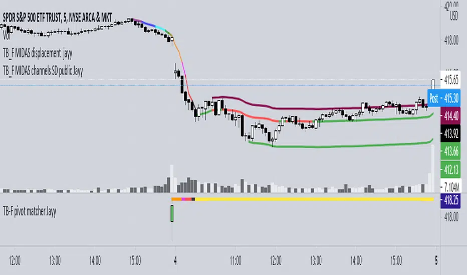
Topfinder Bottomfinder pivot matcher Midas- jayyMidas Technical Analysis: A VWAP Approach to Trading and Investing in Today’s Markets by
Andrew Coles, David G. Hawkins Copyright © 2011 by Andrew Coles and David G. Hawkins.
Appendix C: TradeStation Code for the MIDAS Topfinder/Bottomfinder Curves ported to tradingview
This code is used to assist in adjusting D volume to intersect pivot candle at a pivot candle when using this script: Top Bottom Finder Public version- Jayy found here:
The "n" number entered into the TB-F script is the topfinder/bottomfinder starting point or anchor
Be sure to enter the correct number in the "Topfinder bottomfinder initiation/anchor candle: 1 for CANDLE low - top finder, 2 for CANDLE high - bottom finder, 3 for CANDLE MIDPOINT (hl2) dialogue box
The location of the match point of the pivot candle is extremely important in the: "Match to PIVOT CANDLE: use 1 for CANDLE low, 2 for midtail of the candle below the BODY, 3 for candle BODY low, 4 for CANDLE HIGH, 5 for midpoint of candletail above body, 6 for candle BODY high". Do not
confuse body high with candle high. The body low will either be the candle open or close. The body high will be either the open or close.
If you expect a trend up the pivot candle is likely the low of the pivot candle ie 1 (2 and 3 are alternatives).
In a trend down the high of the pivot candle is often selected ie 4 (5 or 6 are alternatives)
If the candle body is aqua increase D volume if it is orange reduce D volume. Adjust iteratively until the candle body turns yellow. That will mean that the TB-F line passes through the pivot candle at the selected point.
Jayy
Vix FIX / StochRSI StrategyThis strategy is based off of Chris Moody's Vix Fix Indicator . I simply used his indicator and added some rules around it, specifically on entry and exits.
Rules :
Enter upon a filtered or aggressive entry
If there are multiple entry signals, allow pyramiding
Exit when there is Stochastic RSI crossover above 80
This works great on a number of stocks. I am keeping a list of stocks with decent Profit Factors and clean equity curves here .
Possible ways to use this:
Modify this script and setup alerts around the various entries
Use as is with different stocks or currency pairs
Modify entry / exit points to make it more profitable for even more symbols and currencies

UCS_Squeeze_Timing-V1There is an important information the Squeeze indicator is missing, which is the Pre Squeeze entry. While the Bollinger band begins to curves out of the KC, The breakout usually happens. There are many instances that the Squeeze indicator will fire, after the Major move, I cant blame the indicator, thats the nature (lagging) of all indicators, and we have to live with it.
Therefore pre-squeeze-fire Entry can be critical in timing your entry. Timing it too early could result in stoploss if it turns against you, ( or serious burn on options premium), because we never know when the squeeze will fire with the TTM squeeze, But now We know. Its a little timing tool. Managing position is critical when playing options.
I will code the timing signal when I get some time.
Updated Versions -
XAUUSD 1-Minute Scalping Strategy - Advanced Strategy for ExitsThis is a **mean-reversion scalping strategy** optimized for **XAUUSD on the 1-minute (or the 5-minute) timeframe**. It combines a classic **RSI(14)** oscillator with an optional **200-period EMA trend filter** to identify short-term overextended conditions in gold price action, while enforcing fixed, conservative exits to maintain strict risk control.
### Core Logic & Why This Combination:
The strategy enters counter-trend when RSI reaches extreme levels (below 30 for longs, above 70 for shorts), capturing quick snap-backs that frequently occur in gold's intraday volatility.
- **RSI(14)** acts as the primary momentum filter — detecting oversold/overbought exhaustion.
- The **200 EMA trend filter** (enabled by default) adds directional context: longs are allowed only when price is above the EMA (overall uptrend bias), shorts only below it (downtrend bias). This reduces whipsaws in strong trending sessions and improves trade quality without overly restricting opportunities.
- Disabling the trend filter allows pure mean-reversion trading (useful in ranging/Asian sessions), but enabling it is strongly recommended for better expectancy in most market conditions.
Entries occur only when flat (no pyramiding), keeping the system clean and directional.
### Exit Rules (Fixed at Entry):
- **Take Profit**: +10 pips (0.10 in XAUUSD price terms)
- **Stop Loss**: -5 pips (0.05 in price terms)
- **Risk:Reward** = 1:2
Exits are **set once on the entry bar** using limit/stop orders — this prevents dynamic recalculation and mimics real broker behavior more closely. The 2:1 RR gives the strategy mathematical edge even with moderate win rates.
### Performance & Realism Guidelines:
This strategy is tuned for **high-frequency scalping** on gold, which typically produces hundreds to thousands of trades per year on 1-minute data.
Recommended **backtest/publication settings** (update these in the strategy properties before publishing):
- **Initial Capital**: $10,000 – $50,000 (realistic for retail prop/swing traders; the script defaults to $1,000,000 only for visual scaling — change it!)
- **Order Size**: Fixed 0.10–0.50 lots (adjust according to account size)
- **Commission**: 3–7 USD per round-turn lot (typical ECN/raw-spread gold commission on brokers like IC Markets, Pepperstone, etc.)
- **Slippage**: 2–5 ticks (≈0.02–0.05 in price) — gold can be slippery during news/volatility spikes on 1-minute charts
- **Pyramiding**: 1 (default — no stacking)
- **Dataset**: At minimum 1–3 years of 1-minute data (aim for >500–1000 closed trades for statistical significance)
With realistic costs applied, expect win rate ≈55–70%, profit factor >1.4–1.8 in favorable periods, but results vary significantly across trending vs. ranging regimes and news events.
**Risk per trade** remains very controlled (typically <0.5–1.5% depending on SL distance and position sizing) — never exceeds sustainable levels.
### Important Usage Notes:
- Check thoroughly the curve-fitted back tests.
- Gold is extremely volatile on 1-minute charts; check major news (NFP, FOMC, FED) unless you widen SL/TP dynamically (you can manually implement it here).
- Always forward-test on demo first and use proper position sizing.
- The built-in dashboard shows live stats (net P&L, win rate, profit factor, current RSI, position status, etc.) for quick monitoring.
- Restricted Sample Size for Precision
Happy scalping — trade responsibly! 🚀

Auction Weighted Support and Resistance [Metrify]This script builds an “auction-weighted” S/R map that’s intentionally closer to a microstructure proxy than a classic “draw pivots → draw lines” approach.
The core idea: treat repeated interactions around the same price as evidence of auction behavior (acceptance vs rejection), then compress that behavior into a small set of ranked horizontal zones per horizon. Instead of outputting dozens of levels, it runs a selection pass to keep only the strongest, spatially distinct levels.
Candidate discovery is pivot-driven, but not used naively. The script collects pivot highs/lows into rolling buffers for three horizons (Micro/Short/Medium) with different pivot lengths and memory caps. Those candidates don’t become “levels” directly; they’re just seeds that get clustered and rescored. Clustering is ATR-normalized (distance measured in ATR multiples), so the same logic doesn’t fall apart when you change symbol volatility or timeframe. Each horizon has its own clustering radius (distATR_micro/short/medium), which makes Micro more granular and Medium more tolerant.
The “weight” you see is not a single metric. It’s a composite score that tries to approximate how meaningful a price is in an auction sense:
Touch count (distinct): interactions are counted only when the candle range gets within a near-band threshold (ATR-normalized), and then gated by minimum bar separation so you don’t get spam from chop printing 20 touches in a row. (this is done with a stride-based loop to avoid blowing runtime on deep lookbacks)
Acceptance: a rolling overlap rate of candle ranges inside the box. It’s exponentially weighted (half-life decay), so recent acceptance matters more, but older acceptance still contributes. If price has been “living” around that level, acceptance rises.
Rejection quality: wick-aware rejection, but range-gated (not close-gated). The scoring looks at whether the candle range overlaps/approaches the level, then measures wick dominance on the rejecting side plus where the close sits inside the bar range.
Age decay: older levels aren’t thrown away automatically, but they get downweighted via an exponential decay term so stale structure doesn’t dominate forever.
Those components get combined by f_weightCompose() into a bounded weight using saturating transforms (so touches don’t scale linearly forever) and a decay factor tied to age. When multiple candidates land in the same cluster, the merge is done with a saturating union on weights (1 - (1-oldW)*(1-wAdd)) rather than simple addition, so weights don’t explode and a level can converge toward 1.0 without becoming meaningless. The cluster center price is updated via a weight-based average to prevent random drift from weak additions.
After clustering, we does an explicit selection pass instead of drawing everything. First it filters by minScore, then sorts by weight, then applies a spatial suppression step (basically NMS for horizontal levels). The minimum spacing is ATR-based and incorporates both a horizon spacing floor and the zone thickness, so you don’t end up with two bands that overlap visually or convey the same information. On top of that, there’s a global cross-horizon collision gate (f_canDraw) so Medium zones can coexist with Short/Micro without the chart turning into a layered fog of rectangles.
Visualization is intentionally “zone-first.” Each selected level becomes a box band whose half-thickness is ATR-scaled per horizon (bandThicknessATR_*). Opacity isn’t linear: it normalizes weight above minScore, applies a power curve to compress mid-range values, and also scales relative to the strongest level in that horizon (so you still get contrast when everything is “kind of strong”).
The pressure overlay is not volume-based and not orderflow (pine can’t read L2), but it tries to expose short-term imbalance while price is inside a band. When the last price is inside a zone, it computes a pressure score from two parts: proximity to the center (closer = higher) and a directional imbalance proxy from recent returns sampled only on bars that intersect the band. It then draws two thin lines at the band edges with alpha proportional to that pressure score. This is meant as a “are we being pushed out or absorbed here” hint (not a prediction engine).
If you enable the audit panel, the script builds a table listing the levels that actually got drawn (post-selection + collision filtering). The columns map directly to the internal metrics (weight, touches, acceptance, rejection), so you can sanity-check why a level exists. Level IDs are horizon-prefixed (MC/ST/MD) and assigned based on ranking within each horizon.
note:
rebuild is throttled (rebuildEveryN) and only runs on the last bar. Loops that can go deep use a stride heuristic (1/2/4) to keep runtime predictable on large lookbacks. Arrays are used as bounded buffers for candidate storage, and drawing objects are aggressively deleted/rebuilt to avoid object leaks.

Market Cycle Strength# Market Cycle Strength (MCS)
## Overview
Market Cycle Strength is a comprehensive composite indicator that synthesizes six key market health metrics into a single score ranging from -100 to +100. The indicator is designed to help traders assess the current market regime and identify potential turning points by analyzing multiple dimensions of market structure simultaneously.
## How It Works
### Components
The indicator combines six distinct market signals, each weighted by default as follows:
| Component | Weight | What It Measures |
|-----------|--------|------------------|
| **Momentum (30%)** | Price trend strength via SPY's position relative to 50/200 SMAs, golden/death cross status, and rate of change |
| **Credit Spreads (20%)** | Risk appetite through HYG/LQD ratio (high yield vs investment grade bonds) |
| **VIX Structure (20%)** | Fear/greed levels and volatility regime |
| **Market Breadth (15%)** | Participation via RSP/SPY ratio (equal weight vs cap weight performance) |
| **Sector Rotation (10%)** | Leadership patterns by comparing cyclical sectors (XLK, XLY, XLF, XLI, XLB) against defensive sectors (XLU, XLP, XLV, XLRE) |
| **Yield Curve Proxy (5%)** | Flight-to-safety signals via TLT/SHY ratio |
### Score Interpretation
The composite score maps to six market regimes:
- **Strong Bull (+50 to +100)**: Broad strength across most components - healthy expansion
- **Bull (+25 to +50)**: Generally positive conditions with some caution areas
- **Weak Bull (0 to +25)**: Positive but deteriorating - correction risk rising
- **Neutral (-25 to 0)**: Mixed signals - unclear direction, increased caution warranted
- **Bear (-50 to -25)**: Multiple stress indicators present - defensive posture recommended
- **Strong Bear (-100 to -50)**: Significant market stress - crisis conditions
### Contrarian Application
Historical backtesting suggests this indicator has **contrarian value** at extremes:
- Extremely bearish readings (below -25) have historically preceded above-average forward returns
- Very bullish readings (above +70) may indicate complacency rather than a buy signal
The dashboard displays a "CONTRARIAN: BUY SIGNAL" when the score drops below -25, highlighting potential accumulation opportunities.
## How To Use
### Setup
1. Apply the indicator to any chart but SPY is recommended (it fetches all required data via `request.security`)
2. The indicator works best on daily timeframes for regime analysis
3. Adjust component weights in settings if you want to emphasize certain signals
### Dashboard
The table displays:
- **Composite Score**: Overall market health reading
- **Regime**: Current market classification
- **Component Breakdown**: Individual scores for each of the six inputs
- **Status Flags**: Golden/Death cross, credit health, sector leadership, etc.
### Alerts
Four alert conditions are available:
- **Strong Bull Entry**: Score crosses above +50
- **Bear Warning**: Score crosses below -25
- **Contrarian Buy Signal**: Extreme bearish reading (potential opportunity)
- **Regime Change**: Any transition between market regimes
## Best Practices
1. **Context Matters**: Use alongside price action and other analysis - no indicator works in isolation
2. **Timeframe**: Most reliable on daily charts; intraday may produce noise
3. **Extremes Are Signals**: Pay special attention when the score reaches extreme levels in either direction
4. **Component Analysis**: Check individual components to understand what's driving the composite score
5. **Confirmation**: Wait for regime changes to be confirmed by multiple components, not just one
## Inputs
- **Component Weights**: Customize the importance of each signal (default weights sum to 1.0)
- **Show Dashboard**: Toggle the information table on/off
- **Show Zone Background**: Toggle colored zone fills
- **Table Position**: Move dashboard to any corner
- **Alert Thresholds**: Customize notification trigger levels
## Data Sources
The indicator pulls data from:
- SPY, RSP (market proxies)
- HYG, LQD (credit markets)
- TLT, SHY (bond markets)
- VIX (volatility)
- XLK, XLY, XLF, XLI, XLB (cyclical sectors)
- XLU, XLP, XLV, XLRE (defensive sectors)
## Limitations
- Requires access to US market data (best results with TradingView's data feeds)
- Historical data needed for SMA calculations (200+ bars minimum)
- VIX term structure (VIX3M) not available on TradingView, so that component is omitted
- Works best as a daily regime indicator, not for intraday timing
## Acknowledgments
This indicator synthesizes concepts from multiple areas of market analysis including momentum trading, credit cycle research, volatility analysis, and sector rotation theory. The composite approach aims to provide a holistic view of market conditions rather than relying on any single metric.
---
**Disclaimer**: This indicator is for educational and informational purposes only. It does not constitute financial advice. Past performance of any methodology is not indicative of future results. Always conduct your own research and consider your risk tolerance before making trading decisions.

DafeSPALibDafeSPALib: The Shadow Portfolio Adaptation & Strategy Selection Engine
This is not a backtester. This is a live, adaptive portfolio manager. It is a reinforcement learning system that learns which of your strategies to trust in the ever-changing chaos of the market.
█ CHAPTER 1: THE PHILOSOPHY - BEYOND A SINGLE STRATEGY
The search for a single "holy grail" trading strategy is a fool's errand. No single set of rules can perform optimally in all market conditions. A trend-following system that thrives in a bull run will be decimated by a choppy, range-bound market. A mean-reversion strategy that profits from ranges will be run over by a powerful breakout.
The DafeSPALib (Shadow Portfolio Adaptation Library) was created to solve this fundamental problem. It is built on a powerful principle from modern quantitative finance: instead of searching for one perfect strategy, a truly robust system should intelligently allocate to a portfolio of different strategies, dynamically favoring the one that is currently most effective.
This is not just a concept; it is a complete, production-grade engine built in Pine Script. It allows a developer to run multiple "shadow portfolios"—hypothetical trading accounts for each of your strategies—in parallel, in real time. The library tracks the actual equity curve, win rate, Sharpe ratio, and drawdown of each strategy. It then uses a sophisticated selection algorithm to determine which strategy is the "alpha" in the current market regime and tells you which one to follow. It is an AI portfolio manager that lives on your chart.
█ CHAPTER 2: THE CORE INNOVATIONS - WHAT MAKES THIS A REVOLUTIONARY ENGINE?
This library is not a simple strategy switcher. It is a suite of genuine, academically recognized machine learning and statistical concepts, adapted for the Pine Script environment.
Shadow Portfolio Tracking: This is the heart of the system. For each of your strategy "arms," the library maintains a complete, independent set of performance analytics. It doesn't just keep a simple "score." It tracks every hypothetical trade, calculates real P&L;, and updates a full suite of institutional metrics, including the Sharpe Ratio (risk-adjusted return), Sortino Ratio (downside-risk-adjusted return), Profit Factor , and Maximum Drawdown . This provides a rich, data-driven foundation for all decision-making.
Advanced Selection Algorithms: The library doesn't just pick the strategy with the highest recent win rate. It uses sophisticated, battle-tested algorithms from the "multi-armed bandit" problem in machine learning to solve the critical "explore vs. exploit" dilemma:
Thompson Sampling: The default and most powerful. Instead of just picking the "best" arm, it samples from each arm's learned probability distribution of success (its Beta distribution). This naturally balances "exploitation" (using the strategy that works) with "exploration" (giving less-proven strategies a chance to shine), making it incredibly robust against changing conditions.
Upper Confidence Bound (UCB): A deterministic algorithm that is "optimistic in the face of uncertainty." It favors strategies that have both a high win rate and a high degree of uncertainty (fewer trades), encouraging intelligent exploration.
Epsilon-Greedy: A classic RL algorithm that mostly exploits the best-known strategy but, with a small probability (epsilon), explores a random one to prevent getting stuck on a sub-optimal choice.
Trauma-Based Memory Compression: This is a groundbreaking, proprietary concept. When the market experiences a "regime shock" (a sudden explosion in volatility, a violent trend reversal), a simple learning system can be paralyzed or make catastrophic errors. The SPA engine's "trauma" cycle is an intelligent response. It does not erase all learned knowledge. Instead, it compresses the memory : it preserves the direction of what it has learned (e.g., "Strategy A is generally better than B") but it destroys the confidence. The AI "remembers" its experiences but becomes highly uncertain, forcing it to re-learn and adapt to the new market personality with incredible speed. Think of it like PTSD for an AI: the memory of the event remains, but the trust is shattered.
Multi-Layer Concept Drift Detection: This is the system's "earthquake detector." It is constantly scanning for signs that the market's fundamental character is changing ("concept drift"). It uses three layers of detection— Structural (trend slope changes), Volatility (ATR explosions), and Participation (volume anomalies)—to identify a regime shock and trigger the trauma compression cycle.
█ CHAPTER 3: A DUAL-PURPOSE FRAMEWORK - MODES OF OPERATION
This library, along with its companion DAFE libraries, is designed for ultimate flexibility. As a developer, you have complete freedom to use these tools independently or as a fully integrated system.
MODE 1: STANDALONE ENGINE OPERATION (Independent Power)
The DafeSPALib can be used entirely on its own to build a powerful portfolio-of-strategies indicator without any external ML. This approach is perfect for comparing, validating, and dynamically selecting from your own existing, rule-based trading ideas.
The Workflow:
Your indicator initializes the SPA engine with a set number of "arms" (e.g., 4).
On each bar, you calculate the signals for each of your independent strategies (e.g., an EMA Crossover, an RSI Mean Reversion, a Bollinger Breakout).
You feed this array of signals ( ) into the SPA's feed_signals() function.
The SPA engine updates the shadow portfolio for each of the four strategies based on these signals. You then call the select() function, and the SPA's chosen algorithm (e.g., Thompson Sampling) will return the index of the single strategy arm that it trusts the most right now.
Your indicator's final output signal is the signal from that selected arm.
The Result: A complete, self-contained meta-strategy. Your indicator is no longer just one strategy; it is an intelligent manager that dynamically switches between multiple strategies, adapting to the market by selecting the one with the best real-time, risk-adjusted performance.
MODE 2: BRIDGED SUPER-SYSTEM OPERATION (The Ultimate AI)
This is the pinnacle of the DAFE ecosystem. In this advanced mode, the DafeSPALib acts as the "strategic brain" or "portfolio manager" that is fused with a tactical machine learning engine (like the DafeRLMLLib) via a master communication protocol (the DafeMLSPABridge).
The Workflow:
The ML engine generates proposals.
The Bridge Library translates these proposals into a portfolio of micro-strategies.
The SPA engine (this library) receives this portfolio of signals, tracks their shadow performance, and uses its advanced selection algorithms to choose the single best micro-strategy to follow. This becomes the final trade decision.
The final P&L; from the SPA's selection is then routed back through the Bridge to the ML engine as a highly qualified reward signal for learning.
The Result: A hybrid intelligence that is more robust and adaptive than either system alone. The ML provides tactical creativity, while the SPA provides ruthless, performance-based strategic oversight.
█ CHAPTER 4: THE DEVELOPER'S MASTERCLASS - IMPLEMENTATION GUIDE
This library is a professional framework. This guide provides the complete, unabridged instructions and templates required to integrate the DAFE SPA engine into your own custom Pine Script indicators.
PART I: THE INPUTS TEMPLATE (THE CONTROL PANEL)
To give your users full control over the AI, copy this entire block of inputs into your indicator script. It is professionally organized with groups and detailed tooltips.
// ╔════════════════════════════════════════════════════════╗
// ║ INPUTS TEMPLATE (COPY INTO YOUR SCRIPT) ║
// ╚════════════════════════════════════════════════════════╝
// INPUT GROUPS
string G_SPA_ENGINE = "════════════ 🧠 SPA ENGINE ════════════"
string G_SPA_DRIFT = "════════════ 🌊 CONCEPT DRIFT ══════════"
string G_SPA_DASH = "════════════ 📋 DIAGNOSTICS ═══════════"
// SPA ENGINE
int i_spa_num_arms = input.int(4, "Number of Strategy Arms", minval=2, maxval=10, group=G_SPA_ENGINE,
tooltip="The number of parallel strategies the SPA will track.")
string i_spa_selection = input.string("Thompson Sampling", "🤖 Selection Algorithm",
options= , group=G_SPA_ENGINE,
tooltip="The machine learning algorithm used to select the best arm.\n\n" +
"• Thompson Sampling: Bayesian approach, samples from each arm's success probability. Balances explore/exploit perfectly (Recommended).\n" +
"• UCB: Optimistic approach that favors arms with high uncertainty. Excellent for exploration.\n" +
"• Epsilon-Greedy: Mostly exploits the best arm, but explores randomly with a small probability (epsilon).\n" +
"• Softmax: Selects arms based on a probability distribution weighted by their performance.")
float i_spa_epsilon = input.float(0.15, "🧭 Epsilon (for Epsilon-Greedy)", minval=0.01, maxval=0.5, step=0.01, group=G_SPA_ENGINE,
tooltip="The probability of taking a random action to explore. This value automatically decays over time.")
float i_spa_decay = input.float(0.995, "🧠 Memory Decay Rate", minval=0.98, maxval=0.9999, step=0.0005, group=G_SPA_ENGINE,
tooltip="Controls recency bias. A value of 0.995 means the AI gives slightly more weight to recent performance. Lower values create a very short-term memory.")
// CONCEPT DRIFT & TRAUMA
bool i_spa_use_drift = input.bool(true, "🌊 Enable Concept Drift & Trauma", group=G_SPA_DRIFT,
tooltip="Allows the engine to detect market regime shocks and trigger a 'Trauma Compression' cycle to accelerate re-learning.")
float i_spa_trauma_sens = input.float(2.0, "Trauma Sensitivity", minval=1.2, maxval=4.0, step=0.1, group=G_SPA_DRIFT,
tooltip="How sensitive the shock detector is. A lower value will trigger trauma cycles more frequently on smaller volatility/volume spikes.")
// DIAGNOSTICS
bool i_spa_show_dash = input.bool(true, "📋 Show Diagnostics Dashboard", group=G_SPA_DASH)
PART II: THE IMPLEMENTATION LOGIC (THE HEART OF YOUR SCRIPT)
This is the boilerplate code you will adapt to your indicator. It shows the complete loop of feeding signals, detecting drift, and selecting the best strategy.
// ╔═══════════════════════════════════════════════════════╗
// ║ USAGE EXAMPLE (ADAPT TO YOUR SCRIPT) ║
// ╚═══════════════════════════════════════════════════════╝
// 1. INITIALIZE THE ENGINE (happens only on the first bar)
int sel_method_id = i_spa_selection == "Thompson Sampling" ? 0 : i_spa_selection == "Upper Confidence Bound (UCB)" ? 1 : i_spa_selection == "Epsilon-Greedy" ? 2 : 3
var spa.SPAEngine engine = spa.init(
num_arms = i_spa_num_arms,
arm_names = array.from("TrendArm", "ReversionArm", "BreakoutArm", "MomentumArm"), // Give your arms names!
selection_method = sel_method_id,
decay_rate = i_spa_decay,
trauma_sensitivity = i_spa_trauma_sens,
epsilon = i_spa_epsilon
)
// 2. DEFINE YOUR STRATEGY SIGNALS (runs on every bar)
// These are your own custom, rule-based strategies. The signal should be +1 for Buy, -1 for Sell, 0 for Neutral.
int trend_signal = close > ta.ema(close, 200) and ta.crossover(ta.ema(close, 20), ta.ema(close, 50)) ? 1 :
close < ta.ema(close, 200) and ta.crossunder(ta.ema(close, 20), ta.ema(close, 50)) ? -1 : 0
int reversion_signal = ta.crossunder(ta.rsi(close, 14), 30) ? 1 : ta.crossover(ta.rsi(close, 14), 70) ? -1 : 0
int breakout_signal = ta.crossover(close, ta.highest(high, 20) ) ? 1 : ta.crossunder(close, ta.lowest(low, 20) ) ? -1 : 0
int momentum_signal = ta.crossover(ta.mom(close, 10), 0) ? 1 : ta.crossunder(ta.mom(close, 10), 0) ? -1 : 0
// Create an array of your signals. The order MUST be consistent.
array all_signals = array.from(trend_signal, reversion_signal, breakout_signal, momentum_signal)
// 3. THE MAIN LOOP (Feed -> Detect -> Select) - runs on every bar
// --- FEED: Update the shadow portfolios with the latest signals and price ---
engine := spa.feed_signals(engine, all_signals, close)
// --- DETECT: Run the concept drift engine ---
if i_spa_use_drift
float trend_slope = ta.linreg(close, 20, 0) - ta.linreg(close, 20, 1)
engine := spa.detect_drift(engine, close, volume, ta.atr(14), trend_slope)
engine := spa.apply_trauma_cycle(engine) // This will compress memory if a shock was detected
// --- SELECT: Ask the engine for its best choice ---
= spa.select(engine)
engine := updated_engine // CRITICAL: Always update the engine state
// --- ACT: Use the final, selected signal for your indicator's logic ---
int final_signal = array.get(all_signals, selected_arm)
string selected_name = spa.get_name(engine, selected_arm)
// Example: Color bars based on the final, SPA-vetted signal
barcolor(final_signal == 1 ? color.new(color.green, 70) : final_signal == -1 ? color.new(color.red, 70) : na)
// 4. DISPLAY DIAGNOSTICS
if i_spa_show_dash and barstate.islast
string diag_text = spa.diagnostics(engine)
label.new(bar_index, high, diag_text,
style=label.style_label_down,
color=color.new(#0A0A14, 10),
textcolor=#00E5FF,
size=size.small,
textalign=text.align_left)
█ DEVELOPMENT PHILOSOPHY
The DafeSPALib was born from the realization that market adaptation is the true holy grail of trading. While any single strategy is brittle, a portfolio of strategies, managed by an intelligent selection algorithm, is antifragile—it can learn, adapt, and potentially thrive in the face of chaos. This library is an open-source tool for the systems thinker, the quantitative analyst, and the professional developer. It is designed to provide the foundational architecture for building the most robust, adaptive, and intelligent trading systems on the TradingView platform.
This library is a tool for that wisdom. It is not about having the single smartest algorithm, but about having a disciplined, data-driven process for selecting the one that is working right now.
█ DISCLAIMER & IMPORTANT NOTES
THIS IS A LIBRARY FOR ADVANCED DEVELOPERS: This script does nothing on its own. It is a powerful engine that must be integrated into other indicators and fed with valid strategy signals.
PERFORMANCE IS HYPOTHETICAL: The shadow portfolio tracking is a simulation. It does not account for slippage, fees (unless manually added to P&L;), or the psychological pressure of live trading.
LEARNING REQUIRES DATA: The selection algorithms require a sufficient number of trades (at least 20-30 per arm) to make statistically meaningful decisions. The engine will be less reliable during the initial "warm-up" period.
"You don't need to be a rocket scientist. Investing is not a game where the guy with the 160 IQ beats the guy with the 130 IQ."
— Warren Buffett
Taking you to school. - Dskyz, Create with RL.

Multi Trendlines from Pivots (>=3 Touches). DaliliIndicator Description
Multi Trendlines from Pivots (≥3 Touches)
This indicator automatically identifies and draws straight support and resistance trendlines based on confirmed price pivots. It is designed to approximate how a disciplined discretionary trader would draw trendlines, but does so algorithmically and consistently.
What it does
1. Pivot-based structure detection
The indicator first identifies swing highs and swing lows using a configurable pivot length. Only confirmed pivots are used, so lines do not repaint.
2. Line construction logic
For each side of the market:
• Pivot highs are used to construct resistance lines (drawn in red).
• Pivot lows are used to construct support lines (drawn in green).
All possible straight lines formed by pairs of pivots are evaluated.
3. Minimum touch requirement
A line is only considered valid if at least 3 pivot points fall on or very near that line. “Near” is defined by a volatility-adjusted tolerance using ATR (Average True Range), so the logic adapts across symbols and timeframes.
4. Multi-line output
The script does not stop at a single trendline. It draws as many valid lines as possible, up to a configurable maximum per side, prioritizing lines with the highest number of touches.
5. Dynamic updating
Lines are rebuilt only when new pivots form. Old lines are removed and replaced as structure evolves, keeping the chart clean and relevant.
Visual output
• Red straight lines: Resistance lines derived from pivot highs.
• Green straight lines: Support lines derived from pivot lows.
• Lines optionally extend to the right, projecting future support or resistance.
What it is not
• It does not curve or smooth lines.
• It does not use regression channels or moving averages.
• It does not rely on candle bodies unless explicitly modified.
• It does not repaint past structure.
Use case
This indicator is best suited for:
• Structural market analysis.
• Identifying confluence zones where multiple trendlines cluster.
• Swing trading and breakout/failure analysis.
• Overlaying objective structure on discretionary price action analysis.
If you want to further constrain it, the next logical refinements would be:
• Only downward-sloping resistance and upward-sloping support.
• Requiring touches to be higher highs or lower lows.
• Switching touches from pivots to raw candle highs/lows.
• Enforcing minimum bar separation between touches.
All of those can be layered on without changing the core architecture.
