Becak I-series: Indicator Floating Panels v.80Becak I-series: Floating Panels v.80th (Indonesia Independence Days)
What it does:
This indicator creates three floating overlay panels that display MACD, RSI, and Stochastic oscillators directly on your price chart. Unlike traditional separate panes, these panels hover over your chart with customizable positioning and transparency, providing a clean, space-efficient way to monitor multiple technical indicators simultaneously.
When to use:
When you need to monitor momentum, trend strength, and overbought/oversold conditions without cluttering your workspace
Perfect for traders who want quick visual access to multiple oscillators while maintaining focus on price action
Ideal for any timeframe and asset class (stocks, crypto, forex, commodities)
How it works:
The script calculates standard MACD (12,26,9), RSI (14), and Stochastic (14,3,3) values, then renders them as floating panels with:
MACD Panel: Shows MACD line (blue), Signal line (orange), and histogram (green/red bars)
RSI Panel: Displays RSI line (purple) with overbought (70) and oversold (30) reference levels
Stochastic Panel: Shows %K (blue) and %D (orange) lines with optional buy/sell signals and highlighted overbought/oversold zones
Customization options:
Position: Choose Top, Bottom, or Auto-Center placement
Size: Adjust panel height (15-35% of chart) and spacing between panels
Positioning: Fine-tune vertical center offset and horizontal positioning
Appearance: Toggle panel backgrounds and adjust transparency (50-95%)
Parameters: Modify all indicator lengths and overbought/oversold levels
Signals: Enable/disable Stochastic crossover signals
Display: Control lookback period (30-100 bars) and right margin spacing
Universal compatibility: Works seamlessly across all asset types with automatic range detection and scaling.
DIRGAHAYU HARI KEMERDEKAAN KE 80 - INDONESIA ... MERDEKA!!!!!
Search in scripts for "forex"

Currency Strength v3.0Currency Strength v3.0
Summary
The Currency Strength indicator is a powerful tool designed to gauge the relative strength of major and emerging market currencies. By plotting the True Strength Index (TSI) of various currency indices, it provides a clear visual representation of which currencies are gaining momentum and which are losing it. This indicator automatically detects the currency pair on your chart and highlights the corresponding strength lines, simplifying analysis and helping you quickly identify potential trading opportunities based on currency dynamics.
Key Features
Comprehensive Currency Analysis: Tracks the strength of 19 currencies, including major pairs and several emerging market currencies.
Automatic Pair Detection: Intelligently identifies the base and quote currency of the active chart, automatically highlighting the relevant strength lines.
Dynamic Coloring: The base currency is consistently colored blue, and the quote currency is colored gold, making it easy to distinguish between the two at a glance.
Non-Repainting TSI Calculation: Uses the True Strength Index (TSI) for smooth and reliable momentum readings that do not repaint.
Customizable Settings: Allows for adjustment of the fast and slow periods for the TSI calculation to fit your specific trading style.
Clean Interface: Features a minimalist legend table that only displays the currencies relevant to your current chart, keeping your workspace uncluttered.
How It Works
The indicator pulls data from major currency indices (like DXY for the US Dollar and EXY for the Euro). For currencies that don't have a dedicated index, it uses their USD pair (e.g., USDCNY) and inverts the calculation to derive the currency's strength relative to the dollar. It then applies the True Strength Index (TSI) to this data. The TSI is a momentum oscillator that is less volatile than other oscillators, providing a more reliable measure of strength. The resulting values are plotted on the chart, allowing you to see how different currencies are performing against each other in real-time.
How to Use
Trend Confirmation: When the base currency's line is rising and above the zero line, and the quote currency's line is falling, it can confirm a bullish trend for the pair. The opposite would suggest a bearish trend.
Identifying Divergences: Look for divergences between the currency strength lines and the price action of the pair. For example, if the price is making higher highs but the base currency's strength is making lower highs, it could signal a potential reversal.
Crossovers: A crossover of the base and quote currency lines can signal a shift in momentum. A bullish signal occurs when the base currency line crosses above the quote currency line. A bearish signal occurs when it crosses below.
Overbought/Oversold Levels: The horizontal dashed lines at 0.5 and -0.5 can be used as general guides for overbought and oversold conditions, respectively. Strength moving beyond these levels may indicate an unsustainable move that is due for a correction.
Settings
Fast Period: The short-term period for the TSI calculation. Default is 7.
Slow Period: The long-term period for the TSI calculation. Default is 15.
Index Source: The price source used for the calculations (e.g., Close, Open). Default is Close.
Base Currency Color: The color for the base currency line. Default is Royal Blue.
Quote Currency Color: The color for the quote currency line. Default is Goldenrod.
Disclaimer
This indicator is intended for educational and analytical purposes only. It is not financial advice. Trading involves substantial risk, and past performance is not indicative of future results. Always conduct your own research and risk management before making any trading decisions.

Candle H-L and C-O PipsPip Value Indicator
Displays whole-number pip distances for forex candles
What it shows:
H-L: The High-Low range in pips
C-O: The Close-Open difference in pips (direction shown via +/-)
Key features:
Auto-detects JPY pairs (uses 0.01 pip size)
All other forex pairs use 0.0001 pip size
Displays only whole numbers (no decimals)
Shows values when hovering over candles
Clean white markers above each bar

VWAP Bands Pro - Session Based by kobiko3030
📊 Advanced Professional Trading Indicator
VWAP Bands Pro is an advanced indicator that combines the power of VWAP with 4 dynamic bands for precise identification of support and resistance zones. This indicator is designed for professional traders who want deep and accurate market movement analysis.
✨ Key Features
🎯 Smart VWAP Bands
4 adjustable bands based on standard deviation
Optional band 4 hiding for beginner traders
Precise calculation based on volume-weighted price
🌏 Global Session Support
New York Session (9:30 EST)
Asia Session (18:00 EST)
Automatic reset at the beginning of each session
📱 Flexible User Interface
Dynamic labels (V, VR1-4, VS1-4)
Custom color selection
Adjustable line thickness for each band
Multiple display modes
🔔 Advanced Alert System
VWAP breakout alerts
Alerts for all bands (3 & 4)
Clear and precise messages
🛠️ Customization Options
Band Settings
Standard deviation multipliers: 1.0, 2.0, 3.0, 4.0 (default)
Each band independently adjustable
Range: 0.1 to 5.0
Display Settings
Continuous trading start - display from session beginning
Limited candle count - show last X candles
Current day only - no historical data
Visual Design
VWAP, support, and resistance colors
Individual line thickness
Hideable labels
📈 Trading Strategies
Support and Resistance Zones
VS1-VS4: Support bands (green)
VR1-VR4: Resistance bands (red)
V: Central VWAP line
Entry Points
Breakouts above/below VWAP
Bounces from outer bands
Band retests
Risk Management
Use bands as Stop Loss levels
Identify oversold/overbought zones
Adapt to different market conditions
🎖️ Indicator Advantages
✅ Precise calculation based on volume weighting
✅ Complete flexibility in customization
✅ Global session support
✅ User-friendly interface
✅ Built-in alert system
✅ Suitable for all trading styles
📋 Usage Instructions
Add the indicator to your chart
Select trading session (New York/Asia)
Adjust bands according to your trading style
Set up alerts for important breakouts
Start trading with precise key zone identification
💡 Trading Tips
Use outer bands to identify extremes
Combine with additional indicators for confirmation
Adjust bands to asset volatility
Follow alerts to spot opportunities
Consider session-specific behavior patterns
🔧 Technical Specifications
Pine Script Version: 5
Overlay: Yes
Timeframe: All timeframes supported
Markets: Suitable for all markets (Forex, Stocks, Crypto, Futures)
Session Support: New York & Asia with EST timezone
Volume Calculation: HLC3 * Volume weighted
📊 What Makes This Different
Unlike standard VWAP indicators, this pro version offers:
Session-based reset for intraday precision
4 customizable bands instead of basic 2
Professional labeling system for quick identification
Advanced alert conditions for all key levels
Flexible display options for different trading approaches
⚡ Performance Features
Efficient calculation - minimal lag
Clean visual design - no chart clutter
Responsive labels - update in real-time
Session breaks - clear visual separation
Volume validation - ensures accurate VWAP calculation
Correlation Heatmap Matrix [TradingFinder] 20 Assets Variable🔵 Introduction
Correlation is one of the most important statistical and analytical metrics in financial markets, data mining, and data science. It measures the strength and direction of the relationship between two variables.
The correlation coefficient always ranges between +1 and -1 : a perfect positive correlation (+1) means that two assets or currency pairs move together in the same direction and at a constant ratio, a correlation of zero (0) indicates no clear linear relationship, and a perfect negative correlation (-1) means they move in exactly opposite directions.
While the Pearson Correlation Coefficient is the most common method for calculation, other statistical methods like Spearman and Kendall are also used depending on the context.
In financial market analysis, correlation is a key tool for Forex, the Stock Market, and the Cryptocurrency Market because it allows traders to assess the price relationship between currency pairs, stocks, or coins. For example, in Forex, EUR/USD and GBP/USD often have a high positive correlation; in stocks, companies from the same sector such as Apple and Microsoft tend to move similarly; and in crypto, most altcoins show a strong positive correlation with Bitcoin.
Using a Correlation Heatmap in these markets visually displays the strength and direction of these relationships, helping traders make more accurate decisions for risk management and strategy optimization.
🟣 Correlation in Financial Markets
In finance, correlation refers to measuring how closely two assets move together over time. These assets can be stocks, currency pairs, commodities, indices, or cryptocurrencies. The main goal of correlation analysis in trading is to understand these movement patterns and use them for risk management, trend forecasting, and developing trading strategies.
🟣 Correlation Heatmap
A correlation heatmap is a visual tool that presents the correlation between multiple assets in a color-coded table. Each cell shows the correlation coefficient between two assets, with colors indicating its strength and direction. Warm colors (such as red or orange) represent strong negative correlation, cool colors (such as blue or cyan) represent strong positive correlation, and mid-range tones (such as yellow or green) indicate correlations that are close to neutral.
🟣 Practical Applications in Markets
Forex : Identify currency pairs that move together or in opposite directions, avoid overexposure to similar trades, and spot unusual divergences.
Crypto : Examine the dependency of altcoins on Bitcoin and find independent movers for portfolio diversification.
Stocks : Detect relationships between stocks in the same industry or find outliers that move differently from their sector.
🟣 Key Uses of Correlation in Trading
Risk management and diversification: Select assets with low or negative correlation to reduce portfolio volatility.
Avoiding overexposure: Prevent opening multiple positions on highly correlated assets.
Pairs trading: Exploit temporary deviations between historically correlated assets for arbitrage opportunities.
Intermarket analysis: Study the relationships between different markets like stocks, currencies, commodities, and bonds.
Divergence detection: Spot when two typically correlated assets move apart as a possible trend change signal.
Market forecasting: Use correlated asset movements to anticipate others’ behavior.
Event reaction analysis: Evaluate how groups of assets respond to economic or political events.
❗ Important Note
It’s important to note that correlation does not imply causation — it only reflects co-movement between assets. Correlation is also dynamic and can change over time, which is why analyzing it across multiple timeframes provides a more accurate picture. Combining correlation heatmaps with other analytical tools can significantly improve the precision of trading decisions.
🔵 How to Use
The Correlation Heatmap Matrix indicator is designed to analyze and manage the relationships between multiple assets at once. After adding the tool to your chart, start by selecting the assets you want to compare (up to 20).
Then, choose the Correlation Period that fits your trading strategy. Shorter periods (e.g., 20 bars) are more sensitive to recent price movements, making them suitable for short-term trading, while longer periods (e.g., 100 or 200 bars) provide a broader view of correlation trends over time.
The indicator outputs a color-coded matrix where each cell represents the correlation between two assets. Warm colors like red and orange signal strong negative correlation, while cool colors like blue and cyan indicate strong positive correlation. Mid-range tones such as yellow or green suggest correlations that are close to neutral. This visual representation makes it easy to spot market patterns at a glance.
One of the most valuable uses of this tool is in portfolio risk management. Portfolios with highly correlated assets are more vulnerable to market swings. By using the heatmap, traders can find assets with low or negative correlation to reduce overall risk.
Another key benefit is preventing overexposure. For example, if EUR/USD and GBP/USD have a high positive correlation, opening trades on both is almost like doubling the position size on one asset, increasing risk unnecessarily. The heatmap makes such relationships clear, helping you avoid them.
The indicator is also useful for pairs trading, where a trader identifies assets that are usually correlated but have temporarily diverged — a potential arbitrage or mean-reversion opportunity.
Additionally, the tool supports intermarket analysis, allowing traders to see how movements in one market (e.g., crude oil) may impact others (e.g., the Canadian dollar). Divergence detection is another advantage: if two typically aligned assets suddenly move in opposite directions, it could signal a major trend shift or a news-driven move.
Overall, the Correlation Heatmap Matrix is not just an analytical indicator but also a fast, visual alert system for monitoring multiple markets at once. This is particularly valuable for traders in fast-moving environments like Forex and crypto.
🔵 Settings
🟣 Logic
Correlation Period : Number of bars used to calculate correlation between assets.
🟣 Display
Table on Chart : Enable/disable displaying the heatmap directly on the chart.
Table Size : Choose the table size (from very small to very large).
Table Position : Set the table location on the chart (top, middle, or bottom in various alignments).
🟣 Symbol Custom
Select Market : Choose the market type (Forex, Stocks, Crypto, or Custom).
Symbol 1 to Symbol 20: In custom mode, you can define up to 20 assets for correlation calculation.
🔵 Conclusion
The Correlation Heatmap Matrix is a powerful tool for analyzing correlations across multiple assets in Forex, crypto, and stock markets. By displaying a color-coded table, it visually conveys both the strength and direction of correlations — warm colors for strong negative correlation, cool colors for strong positive correlation, and mid-range tones such as yellow or green for near-zero or neutral correlation.
This helps traders select assets with low or negative correlation for diversification, avoid overexposure to similar trades, identify arbitrage and pairs trading opportunities, and detect unusual divergences between typically aligned assets. With support for custom mode and up to 20 symbols, it offers high flexibility for different trading strategies, making it a valuable complement to technical analysis and risk management.

Camarilla Levels Pro Camarilla Levels Pro – Precision Intraday & Swing Trading Tool
Unlock the full potential of Camarilla Pivot Levels for identifying high-probability reversal zones, breakout triggers, and intraday bias shifts.
This indicator automatically calculates L1–L5 levels based on the Camarilla formula, updating daily for precise market adaptation. Whether you’re trading futures, forex, stocks, or crypto, you’ll instantly see:
Reversal Zones – Where price historically reacts and traps traders.
Breakout Zones – L4/L5 for bullish breakouts, L3/L2 for bearish reversals.
Bias Shifts – Quickly gauge if the market is leaning long or short.
Custom Alerts – Get notified when price touches or breaks your chosen level.
Features:
Auto-adjusting Camarilla levels for any symbol & timeframe
Color-coded zones for instant visual recognition
Optional mid-levels for scalpers
Fully customizable styling to match your chart setup
Ideal for:
Day traders wanting precision entry/exit zones
Swing traders watching key daily pivot breaks
Scalpers looking for high-probability reaction points
Triple EMA with Alert | 21, 50, 200 EMA Strategy + Crossover🚀 Boost your trading edge with the Triple EMA with Alert — a professional-grade indicator designed for traders who want precise, real-time trend confirmation across short, medium, and long-term market movements.
🔹 What Makes This Indicator Powerful?
Three Adjustable EMAs — Default: 21, 50, 200 periods (fully customizable 1–200).
Toggle Visibility — Show only the EMAs you need for your strategy.
Real-Time Alerts — Get notified instantly when:
EMA 1 crosses EMA 2 → short-term trend change.
EMA 2 crosses EMA 3 → medium-term trend alignment.
Works on All Markets & Timeframes — Forex, crypto, stocks, indices, and commodities.
🔹 Why Traders Love It
📊 Multi-Timeframe Trend Confirmation — Filter out noise and trade with market momentum.
🎯 Accurate Crossover Signals — Identify bullish and bearish momentum shifts.
🔔 Hands-Free Monitoring — Alerts keep you informed even when you’re away from the chart.
💡 Versatile for Any Strategy — Perfect for scalping, swing trading, or long-term investing.
🔹 How to Use It
Bullish Signal — EMA 1 crossing above EMA 2 or EMA 2 crossing above EMA 3.
Bearish Signal — EMA 1 crossing below EMA 2 or EMA 2 crossing below EMA 3.
Combine with support/resistance zones, RSI, or volume for higher probability trades.
📌 Pro Tip:
Use EMA 21 & EMA 50 for momentum confirmation.
Use EMA 200 to spot the overall market direction.
If you’re serious about trend trading with precision, the Triple EMA with Alert will keep you one step ahead of market moves — no more missed entries or exits.
Correlation HeatMap Matrix Data [TradingFinder]🔵 Introduction
Correlation is a statistical measure that shows the degree and direction of a linear relationship between two assets.
Its value ranges from -1 to +1 : +1 means perfect positive correlation, 0 means no linear relationship, and -1 means perfect negative correlation.
In financial markets, correlation is used for portfolio diversification, risk management, pairs trading, intermarket analysis, and identifying divergences.
Correlation HeatMap Matrix Data TradingFinder is a Pine Script v6 library that calculates and returns raw correlation matrix data between up to 20 symbols. It only provides the data – it does not draw or render the heatmap – making it ideal for use in other scripts that handle visualization or further analysis. The library uses ta.correlation for fast and accurate calculations.
It also includes two helper functions for visual styling :
CorrelationColor(corr) : takes the correlation value as input and generates a smooth gradient color, ranging from strong negative to strong positive correlation.
CorrelationTextColor(corr) : takes the correlation value as input and returns a text color that ensures optimal contrast over the background color.
Library
"Correlation_HeatMap_Matrix_Data_TradingFinder"
CorrelationColor(corr)
Parameters:
corr (float)
CorrelationTextColor(corr)
Parameters:
corr (float)
Data_Matrix(Corr_Period, Sym_1, Sym_2, Sym_3, Sym_4, Sym_5, Sym_6, Sym_7, Sym_8, Sym_9, Sym_10, Sym_11, Sym_12, Sym_13, Sym_14, Sym_15, Sym_16, Sym_17, Sym_18, Sym_19, Sym_20)
Parameters:
Corr_Period (int)
Sym_1 (string)
Sym_2 (string)
Sym_3 (string)
Sym_4 (string)
Sym_5 (string)
Sym_6 (string)
Sym_7 (string)
Sym_8 (string)
Sym_9 (string)
Sym_10 (string)
Sym_11 (string)
Sym_12 (string)
Sym_13 (string)
Sym_14 (string)
Sym_15 (string)
Sym_16 (string)
Sym_17 (string)
Sym_18 (string)
Sym_19 (string)
Sym_20 (string)
🔵 How to use
Import the library into your Pine Script using the import keyword and its full namespace.
Decide how many symbols you want to include in your correlation matrix (up to 20). Each symbol must be provided as a string, for example FX:EURUSD .
Choose the correlation period (Corr\_Period) in bars. This is the lookback window used for the calculation, such as 20, 50, or 100 bars.
Call Data_Matrix(Corr_Period, Sym_1, ..., Sym_20) with your selected parameters. The function will return an array containing the correlation values for every symbol pair (upper triangle of the matrix plus diagonal).
For example :
var string Sym_1 = '' , var string Sym_2 = '' , var string Sym_3 = '' , var string Sym_4 = '' , var string Sym_5 = '' , var string Sym_6 = '' , var string Sym_7 = '' , var string Sym_8 = '' , var string Sym_9 = '' , var string Sym_10 = ''
var string Sym_11 = '', var string Sym_12 = '', var string Sym_13 = '', var string Sym_14 = '', var string Sym_15 = '', var string Sym_16 = '', var string Sym_17 = '', var string Sym_18 = '', var string Sym_19 = '', var string Sym_20 = ''
switch Market
'Forex' => Sym_1 := 'EURUSD' , Sym_2 := 'GBPUSD' , Sym_3 := 'USDJPY' , Sym_4 := 'USDCHF' , Sym_5 := 'USDCAD' , Sym_6 := 'AUDUSD' , Sym_7 := 'NZDUSD' , Sym_8 := 'EURJPY' , Sym_9 := 'EURGBP' , Sym_10 := 'GBPJPY'
,Sym_11 := 'AUDJPY', Sym_12 := 'EURCHF', Sym_13 := 'EURCAD', Sym_14 := 'GBPCAD', Sym_15 := 'CADJPY', Sym_16 := 'CHFJPY', Sym_17 := 'NZDJPY', Sym_18 := 'AUDNZD', Sym_19 := 'USDSEK' , Sym_20 := 'USDNOK'
'Stock' => Sym_1 := 'NVDA' , Sym_2 := 'AAPL' , Sym_3 := 'GOOGL' , Sym_4 := 'GOOG' , Sym_5 := 'META' , Sym_6 := 'MSFT' , Sym_7 := 'AMZN' , Sym_8 := 'AVGO' , Sym_9 := 'TSLA' , Sym_10 := 'BRK.B'
,Sym_11 := 'UNH' , Sym_12 := 'V' , Sym_13 := 'JPM' , Sym_14 := 'WMT' , Sym_15 := 'LLY' , Sym_16 := 'ORCL', Sym_17 := 'HD' , Sym_18 := 'JNJ' , Sym_19 := 'MA' , Sym_20 := 'COST'
'Crypto' => Sym_1 := 'BTCUSD' , Sym_2 := 'ETHUSD' , Sym_3 := 'BNBUSD' , Sym_4 := 'XRPUSD' , Sym_5 := 'SOLUSD' , Sym_6 := 'ADAUSD' , Sym_7 := 'DOGEUSD' , Sym_8 := 'AVAXUSD' , Sym_9 := 'DOTUSD' , Sym_10 := 'TRXUSD'
,Sym_11 := 'LTCUSD' , Sym_12 := 'LINKUSD', Sym_13 := 'UNIUSD', Sym_14 := 'ATOMUSD', Sym_15 := 'ICPUSD', Sym_16 := 'ARBUSD', Sym_17 := 'APTUSD', Sym_18 := 'FILUSD', Sym_19 := 'OPUSD' , Sym_20 := 'USDT.D'
'Custom' => Sym_1 := Sym_1_C , Sym_2 := Sym_2_C , Sym_3 := Sym_3_C , Sym_4 := Sym_4_C , Sym_5 := Sym_5_C , Sym_6 := Sym_6_C , Sym_7 := Sym_7_C , Sym_8 := Sym_8_C , Sym_9 := Sym_9_C , Sym_10 := Sym_10_C
,Sym_11 := Sym_11_C, Sym_12 := Sym_12_C, Sym_13 := Sym_13_C, Sym_14 := Sym_14_C, Sym_15 := Sym_15_C, Sym_16 := Sym_16_C, Sym_17 := Sym_17_C, Sym_18 := Sym_18_C, Sym_19 := Sym_19_C , Sym_20 := Sym_20_C
= Corr.Data_Matrix(Corr_period, Sym_1 ,Sym_2 ,Sym_3 ,Sym_4 ,Sym_5 ,Sym_6 ,Sym_7 ,Sym_8 ,Sym_9 ,Sym_10,Sym_11,Sym_12,Sym_13,Sym_14,Sym_15,Sym_16,Sym_17,Sym_18,Sym_19,Sym_20)
Loop through or index into this array to retrieve each correlation value for your custom layout or logic.
Pass each correlation value to CorrelationColor() to get the corresponding gradient background color, which reflects the correlation’s strength and direction (negative to positive).
For example :
Corr.CorrelationColor(SYM_3_10)
Pass the same correlation value to CorrelationTextColor() to get the correct text color for readability against that background.
For example :
Corr.CorrelationTextColor(SYM_1_1)
Use these colors in a table or label to render your own heatmap or any other visualization you need.

Enhanced RSI KDE | Advanced FiltersThis is an enhanced version of the excellent RSI (Kernel Optimized) indicator originally created by @fluxchart. Full credit goes to fluxchart for the innovative KDE (Kernel Density Estimation) concept and the solid foundation that made this enhancement possible.
🙏 CREDITS & ACKNOWLEDGMENTS
Original Creator: @fluxchart - RSI (Kernel Optimized)
Original Concept: Kernel Density Estimation applied to RSI pivot analysis
Enhancement: Advanced filtering system and signal optimization- profitgang
License: Mozilla Public License 2.0
🚀 WHAT'S NEW IN THIS ENHANCED VERSION
Building upon fluxchart's brilliant KDE RSI foundation, this version adds:
🔥 Advanced Filtering System:
Multi-Timeframe Confluence - Confirms signals across higher timeframes
Volume Confirmation - Only signals on above-average volume
Volatility Range Filter - Avoids signals in choppy or extreme conditions
Trend Context Analysis - Considers overall market direction
Adaptive Pivot Detection - Adjusts sensitivity based on market volatility
🎯 Signal Quality Improvements:
Confluence Scoring - Each signal gets a quality score (1-6)
Label Cooldown System - Prevents chart clutter with smart spacing
Higher Activation Thresholds - More selective signal generation
Risk Management Integration - Auto stop-loss and take-profit levels
📊 Enhanced Dashboard:
Real-time filter status monitoring
KDE probability percentages
Confluence scores for both directions
Volume and volatility readings
⚙️ HOW IT WORKS
The indicator maintains fluxchart's core KDE methodology:
Collects RSI values at historical pivot points
Creates probability density functions using Gaussian/Uniform/Sigmoid kernels
Identifies high-probability zones for potential reversals
NEW: Multiple filters must align before generating signals, dramatically reducing false positives while maintaining the accuracy of high-probability setups.
🎛️ RECOMMENDED SETTINGS
Confluence Score: 5/6 (very selective)
Activation Threshold: Medium or High
Multi-Timeframe: Enabled with 2/2 alignment
Volume Filter: Enabled (1.5x threshold)
All other filters: Enabled for maximum quality
📈 BEST USE CASES
Swing Trading - Higher timeframe confirmation reduces whipsaws
Quality over Quantity - Fewer but much higher probability signals
Risk Management - Built-in stop/target levels for each signal
Multi-Asset Analysis - Works on stocks, crypto, forex, commodities
⚠️ IMPORTANT NOTES
This is a quality-focused indicator - expect fewer but better signals
Backtest thoroughly on your specific assets and timeframes
The original fluxchart indicator remains excellent for different trading styles
Consider this an alternative approach, not a replacement
🤝 COLLABORATION & FEEDBACK
Special thanks to @fluxchart for creating the original innovative KDE RSI concept. This enhancement wouldn't exist without that solid foundation.
Feel free to suggest improvements or share your results! The goal is to build upon great work in the community.

WaveTrend Dynamic (Lazy Bear Style)█ OVERVIEW
The WaveTrend Dynamic indicator (in the style of Lazy Bear) is an advanced tool based on the Exponential Smoothing Average (ESA), which adapts to the volatility and price of a financial instrument. It is more flexible than the classic WaveTrend but shares a similar concept of bands around a main oscillator line.
The indicator uses dynamic bands calculated as distances from the ESA, with their width adjustable via the "level" parameter. This allows it to be tailored to various markets, timeframes, and volatility conditions, making it easier to identify trends, reversal points, and buy/sell signals.
█ CONCEPTS
The WaveTrend Dynamic combines oscillator functions with trend analysis. Below, we explain the key components in a simple way, understandable even for beginner users.
Core Calculations
The indicator relies on the adaptive ESA and a few straightforward steps:
1 — ESA (Adaptive Average): Calculated as a smoothed average of the price (from high, low, and close, or HLC3) using the ESA Length parameter (default: 10). This number determines how many past candles are considered in the calculation. The ESA quickly responds to price changes, helping to track trends.
2 — Deviation (D): Measures how much the price deviates from the ESA, factoring in market volatility. This allows the indicator to adapt to different instruments.
3 — Price Distance Indicator (CI): Shows how far the price is from the ESA relative to market volatility. This forms the basis for the main indicator line, reacting to price movements.
4 — WT1 (WaveTrend 1): The main line, smoothing the Price Distance Indicator (CI) with the Average Length parameter (default: 21). It reflects the direction of price movement and momentum.
5 — WT2 (WaveTrend 2): A signal line that further smooths WT1 (with a period of 4). It helps confirm signals through crossovers with WT1.
6 — Bands (UpperBand and LowerBand): These form a dynamic channel around the ESA. Their width depends on the level parameter (default: 100). Wider bands result in fewer but more reliable signals. In the original WaveTrend, the oscillator bands use lower values, such as 50 or 60. To achieve classic oscillator signals (more frequent WT1/WT2 crossovers outside the bands), set the level to 50–60.
Trend Identification
The indicator identifies two types of trends:
• Major Trend: Determined by the position of WT1 relative to the ESA. When WT1 is above the ESA, it indicates a bullish trend. When below, it signals a bearish trend. Line and fill colors reflect this trend.
• Mini-Trend: Based on WT1 and WT2 crossovers. When the lines cross, they change to the same color, signaling short-term changes or reversal points. This is ideal for quick trading decisions.
Visuals and Effects
• WT1 and WT2 Lines: Scaled to price and displayed on the price chart for easier analysis.
• Fills: Between the bands (UpperBand/LowerBand) and between WT1/WT2, with a "wave" effect that adjusts transparency based on the trend (green for bullish, red for bearish).
• Signals: Three types—return-to-band, WT1/WT2 crossovers outside the bands, and crossovers inside the bands. Signals are displayed as triangles with different colors for buy and sell.
█ FEATURES
Detailed features of the indicator, aligned with the order of settings in the script:
• Basic Parameters: ESA Length — controls ESA smoothing; Average Length — affects WT1 responsiveness; level (WT Level) — adjusts band width for signal filtering.
• Display Elements: Options to show/hide ESA, bands, WT1/WT2; customizable colors for lines, fills, and the wave effect.
• Signals: Three signal groups (return-to-band, crossovers outside bands, crossovers inside bands) with display and color customization options.
█ HOW TO USE
1 — Add the indicator to your TradingView chart and adjust parameters: — Increase ESA Length and Average Length for low-volatility markets (e.g., stocks), or decrease for cryptocurrencies or forex. — Set level to 50–60 for classic WaveTrend signals with WT1/WT2 crossovers outside bands. The default value of 100 creates wider bands and fewer signals.
2 — Analyze trends: — Major trend (WT1 vs. ESA) shows the overall market direction. — Mini-trends (WT1/WT2 crossovers) help time short-term entries.
3 — Use signals: — Return-to-band: Buy at the lower band, sell at the upper band (mean-reversion). — Crossovers outside bands: Indicate strong momentum (with a lower level, e.g., 50). — Crossovers inside bands: Signal weaker trend changes.
4 — Combine with other tools: Use with volume, RSI, or support/resistance for better decisions. Test on historical data to optimize settings.

EFXU Banker Level Price GridThe EFXU Banker Level Price Grid indicator draws fixed horizontal price levels at key whole-number intervals for Forex pairs, regardless of zoom level or timeframe. It’s designed for traders who want consistent visual reference points for major and minor price zones across all charts.
Features:
Major 1000-pip zones (bold lines) above and below a fixed origin price (auto-detects 1.00000 for non-JPY pairs and 100.000 for JPY pairs, or set manually).
500-pip median levels (dashed lines) between each major zone.
100-pip subdivisions (dotted lines) within each 1000-pip zone.
Adjustable number of zones above and below the origin.
Customizable colors, line widths, and label sizes.
Optional labels on the right edge for quick zone identification.
Works on all timeframes and stays visible regardless of zoom or price position.
Use case:
This tool is ideal for traders using institutional-level zones, psychological price levels, or “big money” areas for planning entries, exits, and risk management. Perfect for swing traders, position traders, and scalpers who rely on major pip milestones for market structure context.

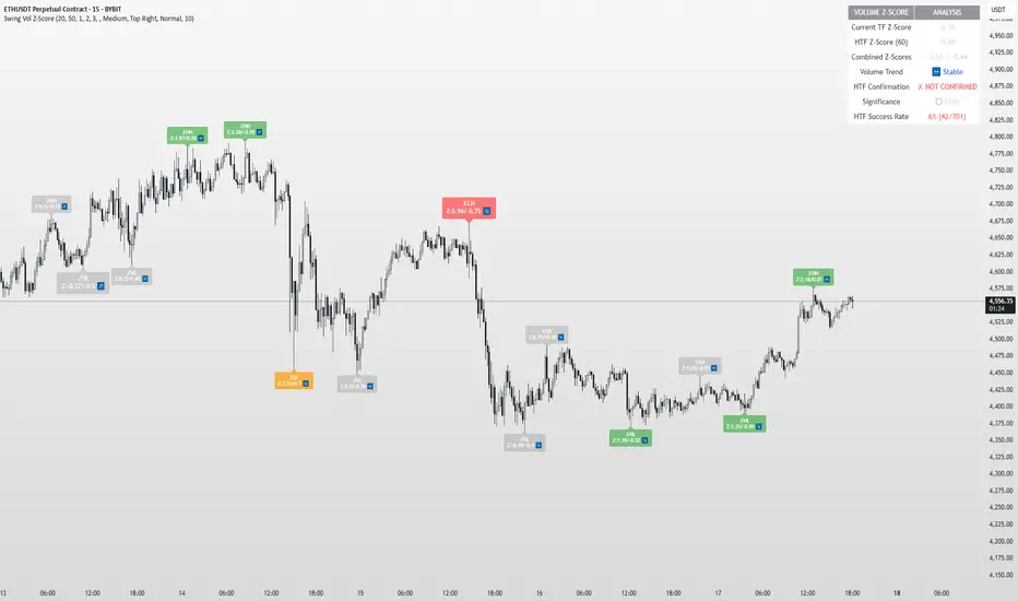
Swing Point Volume Z-ScoreSWING POINT VOLUME Z-SCORE INDICATOR
A volume analysis tool that identifies statistical volume spikes at swing points with optional higher timeframe confirmation.
This indicator uses Leviathan's method of swing detection. All credit to him for his amazing work (and any mistakes mine). I was also inspired by Trading Riot, who's Capitulation indicator gave me the idea to create this one.
WHAT IT DOES
This indicator combines three analytical approaches:
- Volume Z-score calculation to measure volume significance statistically
- Automatic swing point detection (higher highs, lower lows, etc.)
- Optional higher timeframe volume confirmation
The Z-score measures how many standard deviations current volume is from the average, helping identify when volume activity is genuinely elevated rather than relying on visual assessment.
VISUAL SYSTEM
The indicator uses a color-coded approach for quick assessment:
GREEN - Normal Activity (Z-Score 1.0-2.0)
Above-average volume levels
ORANGE - Elevated Activity (Z-Score 2.0-3.0)
High volume activity that may indicate increased interest
RED - Potential Institutional Activity (Z-Score 3.0+)
Very high volume levels that could suggest significant market participation
HIGHER TIMEFRAME CONFIRMATION
When enabled, the indicator checks volume on a higher timeframe:
- Checkmark symbol indicates HTF volume also shows elevation
- X symbol indicates HTF volume doesn't confirm
- Auto-selects appropriate higher timeframe or allows manual selection
KEY FEATURES
Statistical Approach: Uses Z-score methodology rather than arbitrary volume thresholds
Adaptive Thresholds: Can adjust based on market volatility conditions
Swing Focus: Concentrates analysis on structurally important price levels
Volume Trends: Shows whether volume is accelerating or decelerating
Success Tracking: Monitors how often HTF confirmation proves effective
DISPLAY OPTIONS
Basic Mode: Essential features with clean interface
Advanced Mode: Additional customization and analytics
Label Sizing: Four size options to fit different screen setups
Table Position: Moveable info table with transparency control
Custom Colors: Adjustable for different chart themes
PRACTICAL APPLICATIONS
May help identify:
- Volume spikes at support/resistance levels
- Potential accumulation or distribution zones
- Breakout confirmation with volume backing
- Areas where larger market participants might be active
Works on all liquid markets and timeframes, though generally more effective on 15-minute charts and higher.
USAGE NOTES
This is an analytical tool that highlights statistically significant volume events. It should be used as part of a broader analysis approach rather than as a standalone trading system.
The indicator works best when combined with:
- Price action analysis
- Support and resistance identification
- Trend analysis
- Proper risk management
Default settings are designed to work well across most instruments, but users can adjust parameters based on their specific needs and trading style.
TECHNICAL DETAILS
Built with Pine Script v5
Compatible with all TradingView subscription levels
Open source code available for review and learning
Works on stocks, forex, crypto, futures, and other liquid instruments
The statistical approach helps remove some subjectivity from volume analysis, though like all technical indicators, it should be used thoughtfully as part of a complete trading plan.
Zero Lag LSMA 3-Color# Zero Lag LSMA 3-Color Indicator
## Overview
The Zero Lag LSMA (ZLSMA) 3-Color is an advanced trend-following indicator that reduces the lag inherent in traditional Linear Regression Moving Averages (LSMA). This indicator provides clear visual signals through a color-coded system and dot markers to identify trend changes with minimal delay.
## What is Zero Lag LSMA?
Zero Lag LSMA is calculated by applying the Linear Regression Moving Average twice and then compensating for the lag:
1. **First LSMA**: Calculate LSMA of the price data
2. **Second LSMA**: Calculate LSMA of the first LSMA
3. **Zero Lag Calculation**: ZLSMA = LSMA + (LSMA - LSMA2)
This method significantly reduces the delay while maintaining the smoothness of the trend line.
## Features
### Color-Coded Trend System
- **Fluorescent Green** (`RGB(0, 255, 0)`): Uptrend - ZLSMA is rising
- **Fluorescent Red** (`RGB(255, 20, 60)`): Downtrend - ZLSMA is falling
- **Gray**: Sideways/Neutral - No clear directional bias
### Trend Change Markers
- **Tiny dots** appear at the exact moment when the trend direction changes
- **Green dots**: Mark the beginning of an uptrend
- **Red dots**: Mark the beginning of a downtrend
### Customizable Parameters
- **Length**: Period for ZLSMA calculation (default: 20)
- **Line Width**: Thickness of the ZLSMA line (default: 2)
- **Show/Hide Toggle**: Option to display or hide the indicator
## Trading Applications
### Trend Identification
- **Green line**: Look for long opportunities
- **Red line**: Look for short opportunities
- **Gray line**: Consider range-bound strategies
### Entry Signals
- **Dot markers** provide precise entry points when trend changes occur
- Green dots can signal potential buy entries
- Red dots can signal potential sell entries
### Trend Confirmation
- Use ZLSMA color changes to confirm other technical analysis signals
- The reduced lag helps traders enter trends earlier than traditional moving averages
## Advantages Over Traditional Moving Averages
1. **Reduced Lag**: Responds faster to price changes than standard moving averages
2. **Clear Visualization**: Color-coding makes trend direction immediately apparent
3. **Precise Timing**: Dot markers highlight exact trend change moments
4. **Smooth Operation**: Maintains smoothness while reducing whipsaws
## Best Practices
### Timeframe Usage
- Works effectively on all timeframes
- Higher timeframes provide more reliable signals
- Lower timeframes offer more trading opportunities but may have more noise
### Risk Management
- Always use proper stop-loss levels
- Consider the overall market context
- Combine with other technical analysis tools for confirmation
### Settings Optimization
- **Shorter periods** (10-15): More sensitive, faster signals
- **Longer periods** (25-50): More stable, fewer false signals
- **Standard period** (20): Good balance between sensitivity and stability
## Alert Conditions
The indicator includes built-in alert conditions for:
- ZLSMA turning upward (trend change to bullish)
- ZLSMA turning downward (trend change to bearish)
## Compatibility
- **Platform**: TradingView
- **Script Version**: Pine Script v6
- **Chart Type**: Works on all chart types
- **Markets**: Suitable for Forex, Stocks, Crypto, Commodities, and Indices
## Disclaimer
This indicator is for educational and informational purposes only. It should not be considered as financial advice. Always conduct your own research and consider your risk tolerance before making trading decisions. Past performance does not guarantee future results.
LANZ Strategy 6.0🔷 LANZ Strategy 6.0 — NY Session Entry Tool & Multi-Account Risk Manager
LANZ Strategy 6.0 - Is a trading tool designed to help traders plan, execute, and manage operations with a focus on risk management, multi-account handling, and visual clarity.
It works exclusively on the 1-hour timeframe ⏳ and is optimized for the New York market opening dynamics.
🧠 Core Concept
The strategy identifies bullish trading opportunities based on the 09:00 NY candle. Once detected, it automatically calculates and draws:
EP (Entry Price) — The exact level where the trade setup triggers.
SL (Stop Loss) — Based on a customizable percentage of the candle's high–low range or wick extremes.
TP (Take Profit) — Calculated using your chosen Risk–Reward Ratio (e.g., 1:5, 1:3, etc.).
⚙️ Main Features
⏳ Time-Specific Execution
Operates only when the 09:00 NY candle closes bullish.
Ideal for traders who align with the New York Session market structure.
💰 Multi-Account Lot Size Management
Up to 5 independent accounts can be configured with their own capital and risk %, showing the exact lot size to use for each.
📏 Adaptive Risk Control
Supports both Forex and non-Forex assets (indices, gold, oil).
For non-Forex, you can manually define the pip value according to your broker’s specs.
🎨 Visual Trade Map
Automatically plots clean and easy-to-read EP, SL, and TP lines with customizable colors, styles, and thickness.
A floating information panel displays levels, pip distances, and lot sizes.
🔔 Real-Time Alerts
Alerts for:
Entry signal detection.
Stop Loss hit.
Take Profit hit.
Manual close at the defined session end.
📊 Example
If you trade GBPUSD with Account #1 set to $10,000 and 2% risk,
and the 09:00 NY candle closes bullish with SL = 30 pips and RR = 5:1:
EP, SL, and TP levels are drawn instantly.
Risk = $200 (2% of $10,000).
Lot size is calculated automatically.
All details are shown in the on-chart panel.
🛠️ How to Use
Load the indicator on a 1-hour chart.
Configure risk settings and account data.
Wait for the 09:00 NY candle to close bullish.
Use the displayed lot size and levels to execute your trade.
Let the tool alert you for SL, TP, or manual close.
⚠️ Disclaimer:
This script is for educational purposes only. It does not guarantee profits and past performance does not represent future results. Always manage your risk responsibly.
👨💻 Credits:
💡 Developed by: LANZ
🧠 Execution Model & Logic Design: LANZ
📅 Designed for: 1H timeframe and NY-based entries

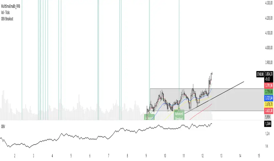
OBV Breakout Screener (By Tarso)1. Purpose of the Indicator
The "Advanced OBV Breakout Screener" is a specialized tool designed to find a powerful bullish signal. It scans for assets where buying pressure is increasing significantly, even though the price has not yet broken out.
The core strategy is to identify assets where:
Volume is leading Price: The On-Balance Volume (OBV) has already broken its recent high.
Price is still contained: The asset's price has not yet broken its recent high.
This setup helps you find potential trading opportunities right before a possible upward move.
2. How to Set Up the Indicator
First, you need to add the script to your TradingView account.
Open any chart on TradingView.
Click on the "Pine Editor" tab at the bottom of the screen.
Delete any existing code and paste the entire "Advanced OBV Breakout Screener" script into the editor.
Click "Add to chart". The indicator will now appear in a separate panel below your main price chart.
3. How to Use it with the Pine Screener (Step-by-Step)
This is the main purpose of the indicator. The script does all the complex analysis and provides a simple "1" (Signal is ON) or "0" (Signal is OFF). You only need to set up one filter.
Open the Stock Screener (or Crypto/Forex Screener).
Click the Filters button to open the settings panel.
Ensure you are on the Pine Screener tab (this allows you to filter using custom indicators).
In the indicator selection menu (it might say "Select Indicator..."), find and choose Advanced OBV Breakout Screener from your list.
Now, configure the single filter condition as follows:
In the first box, select Advanced Breakout Signal.
In the second box, select Equal to.
In the third box, select Number and type 1.
Your filter setup should look clean and simple, like this:
That's it! The screener will now display a list of all assets that currently meet the "Advanced Breakout" criteria for the timeframe you have selected (e.g., Daily, 4h, 1h).
4. Configuring the Lookback Period
By default, the indicator analyzes the last 20 periods. If you want to change this (for example, to scan for breakouts over 50 days), you must adjust it in the indicator's settings on your chart.
Go back to your chart view.
Find the "Advanced OBV Breakout Screener" panel.
Click the Settings icon (⚙️) next to the indicator's name.
In the "Inputs" tab, change the "Lookback Period (days)" to your desired value.
Click "OK".
The Pine Screener will automatically use this new setting for its market scan.
5. Understanding the On-Chart Visuals
When you add the indicator to your chart, you will see:
Blue Line: This is the On-Balance Volume (OBV).
Red Stepped Line: This represents the highest value the OBV has reached during the lookback period. A breakout happens when the blue line moves above this red line.
Green Triangle (▲): This symbol appears below a price candle whenever the full "Advanced Breakout" condition (OBV breakout + Price containment) is met, giving you a clear visual confirmation.
thors_forex_factory_decodingLibrary "forex_factory_decoding"
Supporting Utility Library for the Live Economic Calendar by toodegrees Indicator; responsible for formatting and saving Forex Factory News events.
isLeapYear()
Finds if it's currently a leap year or not.
Returns: Returns True if the current year is a leap year.
daysMonth(M)
Provides the days in a given month of the year, adjusted during leap years.
Parameters:
M (int) : Month in numerical integer format (i.e. Jan=1).
Returns: Days in the provided month.
MMM(M)
Converts a month from a numerical integer format to a MMM format (i.e. 'Jan').
Parameters:
M (int) : Month in numerical integer format (i.e. Jan=1).
Returns: Month in MMM format (i.e. 'Jan').
array2string(S, FWD)
Converts a string array to a simple string, concatenating its elements.
Parameters:
S (array) : String array, or string array slice, to turn into a simple string.
FWD (bool) : Boolean defaulted to True. If True the array will be concatenated from head to tail, reversed order if False.
Returns: Returns the simple string equivalent of the provided string array.
month2number(M)
Converts a month string in 'MMM' format to its integer equivalent.
Parameters:
M (string) : Month string, in 'MMM' format.
Returns: Returns the integer equivalent of the provided Month string in 'MMM' format.
shiftFWD_Days(D)
Shifts forward the current Date by N days.
Parameters:
D (int) : Number of days to forward-shift, default is 7.
Returns: Returns the forward-shifted date in 'MMM %D' format (i.e. Jan 8, Sep 12).
ff_dow(D)
Converts a numbered day of the week string in format to 'DDD' format (i.e. "1" = Sun).
Parameters:
D (string) : Numbered day of the week from 1 to 7, starting on Sunday.
Returns: Returns the day of the week in 'DDD' format (i.e. "Fri").
ff_currency(C)
Converts a numbered currency string in format to 'CCC' format (i.e. "1" = AUD).
Parameters:
C (string) : Numbered currency, where "1" = "AUD", "2" = "CAD", "3" = "CHF", "4" = "CNY", "5" = "EUR", "6" = "GBP", "7" = "JPY", "8" = "NZD", "9" = "USD".
Returns: Returns the currency in 'CCC' format (i.e. "USD").
ff_t(T)
Converts a time of the day in 'hhmm' format into an intger.
Parameters:
T (string) : Time of the day string in 'hhmm' format.
Returns: Returns the time of the day integer in 'hhmm' format, or -1 if all day.
ff_tod(T)
Converts a time of the day from an integer 'hhmm' format into 'hh:mm' format.
Parameters:
T (int)
Returns: Returns the N Forex Factory News array with time of the day string in 'hh:mm' format, or 'All Day'.
ff_impact(I)
Converts a number from 1 to 4 to a relative color based on Forex Factory Impact types.
Parameters:
I (string) : Impact number string from 1 to 4, where "1" = Holiday, "2" = Low Impact, "3" = Medium Impact, "4" = High Impact.
Returns: Returns the color associated to the impact number based on Forex Factory Impact types.
ff_tmst(D, T)
Parameters:
D (string)
T (string)
decode(ID)
Decodes TOODEGREES_FOREX_FACTORY_SLOT_n Symbols' Pine Seeds data into Forex Factory News Events.
Parameters:
ID (int) : Identifier of the Forex Factory News Event, in "DCHHMMI%T" format (D = day of the week from 1 to 7, C = currency from 1 to 9, HHMM = hour:minute in 24h, I = impact from 1 to 4, %T = event title ID) .
Returns: Returns the Forex Factory News Event.
method pullNews(N, n)
Decodes the Forex Factory News Event and adds it to the Forex Factory News array.
Namespace types: array
Parameters:
N (array type from cegb001/forex_factory_utility/1) : Forex Factory News array.
n (float) : imported data from custom feed.
Returns: void
method readNews(N, S)
Pulls the individual Forex Factory News Event from the custom data feed format (joint News string), decodes them and adds them to the Forex Factory News array.
Namespace types: array
Parameters:
N (array type from cegb001/forex_factory_utility/1) : Forex Factory News array.
S (string) : joint string of the imported data from custom feed.
Returns: void

Apex Edge – Liquidity RaiderApex Edge – Liquidity Raider
The Predator That Hunts Where Retail Never Looks
The Liquidity Raider is not your average liquidity line plotter.
This is an institutional-grade hunting system that tracks the pools of liquidity Smart Money algos stalk — and tells you exactly when price is circling in for the strike.
Where most retail tools simply mark lines, this one acts like a predator:
Scans the chart dynamically to detect clustered highs & lows (pivot-based liquidity zones).
Filters noise with sensitivity & price rounding so you only get real liquidity levels — not every random swing.
Plots live BSL (Buy-Side Liquidity) & SSL (Sell-Side Liquidity) lines in clean dotted format.
Auto-deletes levels when swept, so your chart stays clean and focused.
Triggers directional arrows when price comes within your specified % distance to the target liquidity pool — before the market moves.
EMA confluence layer lets you align with institutional flow (customizable Fast & Slow EMAs).
Core Power
Cluster Logic – Finds high-probability liquidity zones using repeated pivot levels.
Sweep Awareness – Lines vanish the moment liquidity is taken, keeping focus on the next pool.
Proximity Strike Detection – Arrow signals only when price is within striking range.
Directional Clarity – Red arrows = targeting BSL, Green arrows = targeting SSL.
Scalable Across Timeframes – Adapts to your chart’s timeframe with dynamic lookback scaling.
Institutional Flow Filter – Optional EMA confirmation keeps you aligned with the real trend.
How to Use
Identify liquidity pools – Dotted green = buy-side, dotted red = sell-side.
Watch proximity arrows – These mean price is in range and hunting that pool.
Align with EMA bias – Enter only in the direction of institutional momentum.
Target the sweep – Your take profit is where the liquidity is resting.
Why Liquidity Raider Wins
This is not a lagging signal system.
It’s a real-time, clean, predictive tool designed to mimic the targeting logic of high-frequency algos.
By removing swept levels and focusing only on the next available pools, Liquidity Raider keeps you one step ahead of the crowd — and perfectly positioned for the kill shot.
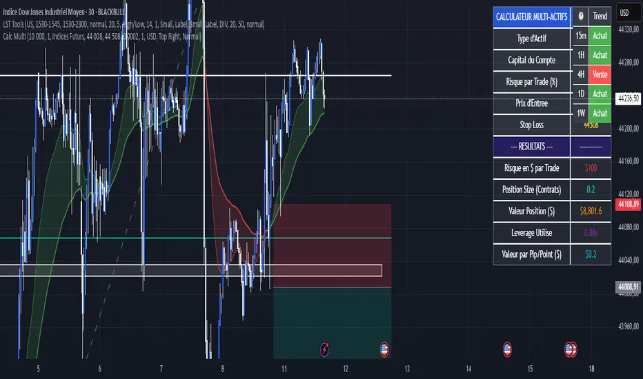
Calculateur Position Size Multi-ActifsThe Multi-Asset Position Size Calculator v6 is a fully customizable Pine Script indicator designed to help you determine the optimal position size based on your risk tolerance across any market: Forex, stocks, crypto, futures indices, or commodities. Features include:
Asset Type Selector: Choose between Forex, Stocks, Crypto, Futures Indices, or Commodities
Account Capital & Risk: Set your total account size and risk percentage per trade
Entry Price & Stop-Loss: Configure your entry and stop-loss levels directly
Automatic or Custom Pip/Point Value: Automatically calculates pip/point value by asset class or enter your own
Contract Size Adjustment: Define contract sizes (e.g., 100,000 units for Forex, 1 for stocks/crypto)
Margin & Leverage Display: View your used leverage and position value in real time
Risk Alerts: Warnings for invalid inputs, high leverage (>10×), and asset-specific risk settings (e.g., crypto leverage)
Integrated Table Interface: On-chart table with adjustable position and text size
Optional Price Level Drawing: Display entry and stop-loss lines on the chart
Trade any market confidently with precise, asset-tailored position sizing and risk management.
Multi-Pip Grid This indicator draws multiple sets of horizontal grid lines on your chart at user-defined pip intervals. It’s designed for traders who want to quickly visualize key price levels spaced evenly apart in pips, with full control over pip size, grid spacing, and appearance.
Features:
Adjustable pip size — works for Forex, gold, crypto, and indices (e.g., 0.0001 for EURUSD, 0.10 for XAUUSD, 1 for NAS100).
Six grid spacings — 1000 pips, 500 pips, 250 pips, 125 pips, 62.5 pips, and 31.25 pips. Each grid can be toggled on or off.
Customizable base price — center the grid at the current market price or any manually entered price.
Optional snap-to-grid — automatically aligns the base price to the nearest multiple of the smallest step for perfect alignment.
Flexible range — choose how many grid lines are drawn above and below the base price.
Distinct colors per grid level for easy identification.
Automatic cleanup — removes old lines before redrawing to avoid clutter.
Use cases:
Identify large and small pip-based support/resistance zones.
Plan entries/exits using fixed pip distances.
Visualize scaled take-profit and stop-loss zones.
Overlay multiple timeframes with consistent pip spacing.
Multi-Pip Grid (Adjustable) — FixedThis indicator draws multiple sets of horizontal grid lines on your chart at user-defined pip intervals. It’s designed for traders who want to quickly visualize key price levels spaced evenly apart in pips, with full control over pip size, grid spacing, and appearance.
Features:
Adjustable pip size — works for Forex, gold, crypto, and indices (e.g., 0.0001 for EURUSD, 0.10 for XAUUSD, 1 for NAS100).
Six grid spacings — 1000 pips, 500 pips, 250 pips, 125 pips, 62.5 pips, and 31.25 pips. Each grid can be toggled on or off.
Customizable base price — center the grid at the current market price or any manually entered price.
Optional snap-to-grid — automatically aligns the base price to the nearest multiple of the smallest step for perfect alignment.
Flexible range — choose how many grid lines are drawn above and below the base price.
Distinct colors per grid level for easy identification.
Automatic cleanup — removes old lines before redrawing to avoid clutter.
Use cases:
Identify large and small pip-based support/resistance zones.
Plan entries/exits using fixed pip distances.
Visualize scaled take-profit and stop-loss zones.
Overlay multiple timeframes with consistent pip spacing.
Kelly Position Size CalculatorThis position sizing calculator implements the Kelly Criterion, developed by John L. Kelly Jr. at Bell Laboratories in 1956, to determine mathematically optimal position sizes for maximizing long-term wealth growth. Unlike arbitrary position sizing methods, this tool provides a scientifically solution based on your strategy's actual performance statistics and incorporates modern refinements from over six decades of academic research.
The Kelly Criterion addresses a fundamental question in capital allocation: "What fraction of capital should be allocated to each opportunity to maximize growth while avoiding ruin?" This question has profound implications for financial markets, where traders and investors constantly face decisions about optimal capital allocation (Van Tharp, 2007).
Theoretical Foundation
The Kelly Criterion for binary outcomes is expressed as f* = (bp - q) / b, where f* represents the optimal fraction of capital to allocate, b denotes the risk-reward ratio, p indicates the probability of success, and q represents the probability of loss (Kelly, 1956). This formula maximizes the expected logarithm of wealth, ensuring maximum long-term growth rate while avoiding the risk of ruin.
The mathematical elegance of Kelly's approach lies in its derivation from information theory. Kelly's original work was motivated by Claude Shannon's information theory (Shannon, 1948), recognizing that maximizing the logarithm of wealth is equivalent to maximizing the rate of information transmission. This connection between information theory and wealth accumulation provides a deep theoretical foundation for optimal position sizing.
The logarithmic utility function underlying the Kelly Criterion naturally embodies several desirable properties for capital management. It exhibits decreasing marginal utility, penalizes large losses more severely than it rewards equivalent gains, and focuses on geometric rather than arithmetic mean returns, which is appropriate for compounding scenarios (Thorp, 2006).
Scientific Implementation
This calculator extends beyond basic Kelly implementation by incorporating state of the art refinements from academic research:
Parameter Uncertainty Adjustment: Following Michaud (1989), the implementation applies Bayesian shrinkage to account for parameter estimation error inherent in small sample sizes. The adjustment formula f_adjusted = f_kelly × confidence_factor + f_conservative × (1 - confidence_factor) addresses the overconfidence bias documented by Baker and McHale (2012), where the confidence factor increases with sample size and the conservative estimate equals 0.25 (quarter Kelly).
Sample Size Confidence: The reliability of Kelly calculations depends critically on sample size. Research by Browne and Whitt (1996) provides theoretical guidance on minimum sample requirements, suggesting that at least 30 independent observations are necessary for meaningful parameter estimates, with 100 or more trades providing reliable estimates for most trading strategies.
Universal Asset Compatibility: The calculator employs intelligent asset detection using TradingView's built-in symbol information, automatically adapting calculations for different asset classes without manual configuration.
ASSET SPECIFIC IMPLEMENTATION
Equity Markets: For stocks and ETFs, position sizing follows the calculation Shares = floor(Kelly Fraction × Account Size / Share Price). This straightforward approach reflects whole share constraints while accommodating fractional share trading capabilities.
Foreign Exchange Markets: Forex markets require lot-based calculations following Lot Size = Kelly Fraction × Account Size / (100,000 × Base Currency Value). The calculator automatically handles major currency pairs with appropriate pip value calculations, following industry standards described by Archer (2010).
Futures Markets: Futures position sizing accounts for leverage and margin requirements through Contracts = floor(Kelly Fraction × Account Size / Margin Requirement). The calculator estimates margin requirements as a percentage of contract notional value, with specific adjustments for micro-futures contracts that have smaller sizes and reduced margin requirements (Kaufman, 2013).
Index and Commodity Markets: These markets combine characteristics of both equity and futures markets. The calculator automatically detects whether instruments are cash-settled or futures-based, applying appropriate sizing methodologies with correct point value calculations.
Risk Management Integration
The calculator integrates sophisticated risk assessment through two primary modes:
Stop Loss Integration: When fixed stop-loss levels are defined, risk calculation follows Risk per Trade = Position Size × Stop Loss Distance. This ensures that the Kelly fraction accounts for actual risk exposure rather than theoretical maximum loss, with stop-loss distance measured in appropriate units for each asset class.
Strategy Drawdown Assessment: For discretionary exit strategies, risk estimation uses maximum historical drawdown through Risk per Trade = Position Value × (Maximum Drawdown / 100). This approach assumes that individual trade losses will not exceed the strategy's historical maximum drawdown, providing a reasonable estimate for strategies with well-defined risk characteristics.
Fractional Kelly Approaches
Pure Kelly sizing can produce substantial volatility, leading many practitioners to adopt fractional Kelly approaches. MacLean, Sanegre, Zhao, and Ziemba (2004) analyze the trade-offs between growth rate and volatility, demonstrating that half-Kelly typically reduces volatility by approximately 75% while sacrificing only 25% of the growth rate.
The calculator provides three primary Kelly modes to accommodate different risk preferences and experience levels. Full Kelly maximizes growth rate while accepting higher volatility, making it suitable for experienced practitioners with strong risk tolerance and robust capital bases. Half Kelly offers a balanced approach popular among professional traders, providing optimal risk-return balance by reducing volatility significantly while maintaining substantial growth potential. Quarter Kelly implements a conservative approach with low volatility, recommended for risk-averse traders or those new to Kelly methodology who prefer gradual introduction to optimal position sizing principles.
Empirical Validation and Performance
Extensive academic research supports the theoretical advantages of Kelly sizing. Hakansson and Ziemba (1995) provide a comprehensive review of Kelly applications in finance, documenting superior long-term performance across various market conditions and asset classes. Estrada (2008) analyzes Kelly performance in international equity markets, finding that Kelly-based strategies consistently outperform fixed position sizing approaches over extended periods across 19 developed markets over a 30-year period.
Several prominent investment firms have successfully implemented Kelly-based position sizing. Pabrai (2007) documents the application of Kelly principles at Berkshire Hathaway, noting Warren Buffett's concentrated portfolio approach aligns closely with Kelly optimal sizing for high-conviction investments. Quantitative hedge funds, including Renaissance Technologies and AQR, have incorporated Kelly-based risk management into their systematic trading strategies.
Practical Implementation Guidelines
Successful Kelly implementation requires systematic application with attention to several critical factors:
Parameter Estimation: Accurate parameter estimation represents the greatest challenge in practical Kelly implementation. Brown (1976) notes that small errors in probability estimates can lead to significant deviations from optimal performance. The calculator addresses this through Bayesian adjustments and confidence measures.
Sample Size Requirements: Users should begin with conservative fractional Kelly approaches until achieving sufficient historical data. Strategies with fewer than 30 trades may produce unreliable Kelly estimates, regardless of adjustments. Full confidence typically requires 100 or more independent trade observations.
Market Regime Considerations: Parameters that accurately describe historical performance may not reflect future market conditions. Ziemba (2003) recommends regular parameter updates and conservative adjustments when market conditions change significantly.
Professional Features and Customization
The calculator provides comprehensive customization options for professional applications:
Multiple Color Schemes: Eight professional color themes (Gold, EdgeTools, Behavioral, Quant, Ocean, Fire, Matrix, Arctic) with dark and light theme compatibility ensure optimal visibility across different trading environments.
Flexible Display Options: Adjustable table size and position accommodate various chart layouts and user preferences, while maintaining analytical depth and clarity.
Comprehensive Results: The results table presents essential information including asset specifications, strategy statistics, Kelly calculations, sample confidence measures, position values, risk assessments, and final position sizes in appropriate units for each asset class.
Limitations and Considerations
Like any analytical tool, the Kelly Criterion has important limitations that users must understand:
Stationarity Assumption: The Kelly Criterion assumes that historical strategy statistics represent future performance characteristics. Non-stationary market conditions may invalidate this assumption, as noted by Lo and MacKinlay (1999).
Independence Requirement: Each trade should be independent to avoid correlation effects. Many trading strategies exhibit serial correlation in returns, which can affect optimal position sizing and may require adjustments for portfolio applications.
Parameter Sensitivity: Kelly calculations are sensitive to parameter accuracy. Regular calibration and conservative approaches are essential when parameter uncertainty is high.
Transaction Costs: The implementation incorporates user-defined transaction costs but assumes these remain constant across different position sizes and market conditions, following Ziemba (2003).
Advanced Applications and Extensions
Multi-Asset Portfolio Considerations: While this calculator optimizes individual position sizes, portfolio-level applications require additional considerations for correlation effects and aggregate risk management. Simplified portfolio approaches include treating positions independently with correlation adjustments.
Behavioral Factors: Behavioral finance research reveals systematic biases that can interfere with Kelly implementation. Kahneman and Tversky (1979) document loss aversion, overconfidence, and other cognitive biases that lead traders to deviate from optimal strategies. Successful implementation requires disciplined adherence to calculated recommendations.
Time-Varying Parameters: Advanced implementations may incorporate time-varying parameter models that adjust Kelly recommendations based on changing market conditions, though these require sophisticated econometric techniques and substantial computational resources.
Comprehensive Usage Instructions and Practical Examples
Implementation begins with loading the calculator on your desired trading instrument's chart. The system automatically detects asset type across stocks, forex, futures, and cryptocurrency markets while extracting current price information. Navigation to the indicator settings allows input of your specific strategy parameters.
Strategy statistics configuration requires careful attention to several key metrics. The win rate should be calculated from your backtest results using the formula of winning trades divided by total trades multiplied by 100. Average win represents the sum of all profitable trades divided by the number of winning trades, while average loss calculates the sum of all losing trades divided by the number of losing trades, entered as a positive number. The total historical trades parameter requires the complete number of trades in your backtest, with a minimum of 30 trades recommended for basic functionality and 100 or more trades optimal for statistical reliability. Account size should reflect your available trading capital, specifically the risk capital allocated for trading rather than total net worth.
Risk management configuration adapts to your specific trading approach. The stop loss setting should be enabled if you employ fixed stop-loss exits, with the stop loss distance specified in appropriate units depending on the asset class. For stocks, this distance is measured in dollars, for forex in pips, and for futures in ticks. When stop losses are not used, the maximum strategy drawdown percentage from your backtest provides the risk assessment baseline. Kelly mode selection offers three primary approaches: Full Kelly for aggressive growth with higher volatility suitable for experienced practitioners, Half Kelly for balanced risk-return optimization popular among professional traders, and Quarter Kelly for conservative approaches with reduced volatility.
Display customization ensures optimal integration with your trading environment. Eight professional color themes provide optimization for different chart backgrounds and personal preferences. Table position selection allows optimal placement within your chart layout, while table size adjustment ensures readability across different screen resolutions and viewing preferences.
Detailed Practical Examples
Example 1: SPY Swing Trading Strategy
Consider a professionally developed swing trading strategy for SPY (S&P 500 ETF) with backtesting results spanning 166 total trades. The strategy achieved 110 winning trades, representing a 66.3% win rate, with an average winning trade of $2,200 and average losing trade of $862. The maximum drawdown reached 31.4% during the testing period, and the available trading capital amounts to $25,000. This strategy employs discretionary exits without fixed stop losses.
Implementation requires loading the calculator on the SPY daily chart and configuring the parameters accordingly. The win rate input receives 66.3, while average win and loss inputs receive 2200 and 862 respectively. Total historical trades input requires 166, with account size set to 25000. The stop loss function remains disabled due to the discretionary exit approach, with maximum strategy drawdown set to 31.4%. Half Kelly mode provides the optimal balance between growth and risk management for this application.
The calculator generates several key outputs for this scenario. The risk-reward ratio calculates automatically to 2.55, while the Kelly fraction reaches approximately 53% before scientific adjustments. Sample confidence achieves 100% given the 166 trades providing high statistical confidence. The recommended position settles at approximately 27% after Half Kelly and Bayesian adjustment factors. Position value reaches approximately $6,750, translating to 16 shares at a $420 SPY price. Risk per trade amounts to approximately $2,110, representing 31.4% of position value, with expected value per trade reaching approximately $1,466. This recommendation represents the mathematically optimal balance between growth potential and risk management for this specific strategy profile.
Example 2: EURUSD Day Trading with Stop Losses
A high-frequency EURUSD day trading strategy demonstrates different parameter requirements compared to swing trading approaches. This strategy encompasses 89 total trades with a 58% win rate, generating an average winning trade of $180 and average losing trade of $95. The maximum drawdown reached 12% during testing, with available capital of $10,000. The strategy employs fixed stop losses at 25 pips and take profit targets at 45 pips, providing clear risk-reward parameters.
Implementation begins with loading the calculator on the EURUSD 1-hour chart for appropriate timeframe alignment. Parameter configuration includes win rate at 58, average win at 180, and average loss at 95. Total historical trades input receives 89, with account size set to 10000. The stop loss function is enabled with distance set to 25 pips, reflecting the fixed exit strategy. Quarter Kelly mode provides conservative positioning due to the smaller sample size compared to the previous example.
Results demonstrate the impact of smaller sample sizes on Kelly calculations. The risk-reward ratio calculates to 1.89, while the Kelly fraction reaches approximately 32% before adjustments. Sample confidence achieves 89%, providing moderate statistical confidence given the 89 trades. The recommended position settles at approximately 7% after Quarter Kelly application and Bayesian shrinkage adjustment for the smaller sample. Position value amounts to approximately $700, translating to 0.07 standard lots. Risk per trade reaches approximately $175, calculated as 25 pips multiplied by lot size and pip value, with expected value per trade at approximately $49. This conservative position sizing reflects the smaller sample size, with position sizes expected to increase as trade count surpasses 100 and statistical confidence improves.
Example 3: ES1! Futures Systematic Strategy
Systematic futures trading presents unique considerations for Kelly criterion application, as demonstrated by an E-mini S&P 500 futures strategy encompassing 234 total trades. This systematic approach achieved a 45% win rate with an average winning trade of $1,850 and average losing trade of $720. The maximum drawdown reached 18% during the testing period, with available capital of $50,000. The strategy employs 15-tick stop losses with contract specifications of $50 per tick, providing precise risk control mechanisms.
Implementation involves loading the calculator on the ES1! 15-minute chart to align with the systematic trading timeframe. Parameter configuration includes win rate at 45, average win at 1850, and average loss at 720. Total historical trades receives 234, providing robust statistical foundation, with account size set to 50000. The stop loss function is enabled with distance set to 15 ticks, reflecting the systematic exit methodology. Half Kelly mode balances growth potential with appropriate risk management for futures trading.
Results illustrate how favorable risk-reward ratios can support meaningful position sizing despite lower win rates. The risk-reward ratio calculates to 2.57, while the Kelly fraction reaches approximately 16%, lower than previous examples due to the sub-50% win rate. Sample confidence achieves 100% given the 234 trades providing high statistical confidence. The recommended position settles at approximately 8% after Half Kelly adjustment. Estimated margin per contract amounts to approximately $2,500, resulting in a single contract allocation. Position value reaches approximately $2,500, with risk per trade at $750, calculated as 15 ticks multiplied by $50 per tick. Expected value per trade amounts to approximately $508. Despite the lower win rate, the favorable risk-reward ratio supports meaningful position sizing, with single contract allocation reflecting appropriate leverage management for futures trading.
Example 4: MES1! Micro-Futures for Smaller Accounts
Micro-futures contracts provide enhanced accessibility for smaller trading accounts while maintaining identical strategy characteristics. Using the same systematic strategy statistics from the previous example but with available capital of $15,000 and micro-futures specifications of $5 per tick with reduced margin requirements, the implementation demonstrates improved position sizing granularity.
Kelly calculations remain identical to the full-sized contract example, maintaining the same risk-reward dynamics and statistical foundations. However, estimated margin per contract reduces to approximately $250 for micro-contracts, enabling allocation of 4-5 micro-contracts. Position value reaches approximately $1,200, while risk per trade calculates to $75, derived from 15 ticks multiplied by $5 per tick. This granularity advantage provides better position size precision for smaller accounts, enabling more accurate Kelly implementation without requiring large capital commitments.
Example 5: Bitcoin Swing Trading
Cryptocurrency markets present unique challenges requiring modified Kelly application approaches. A Bitcoin swing trading strategy on BTCUSD encompasses 67 total trades with a 71% win rate, generating average winning trades of $3,200 and average losing trades of $1,400. Maximum drawdown reached 28% during testing, with available capital of $30,000. The strategy employs technical analysis for exits without fixed stop losses, relying on price action and momentum indicators.
Implementation requires conservative approaches due to cryptocurrency volatility characteristics. Quarter Kelly mode is recommended despite the high win rate to account for crypto market unpredictability. Expected position sizing remains reduced due to the limited sample size of 67 trades, requiring additional caution until statistical confidence improves. Regular parameter updates are strongly recommended due to cryptocurrency market evolution and changing volatility patterns that can significantly impact strategy performance characteristics.
Advanced Usage Scenarios
Portfolio position sizing requires sophisticated consideration when running multiple strategies simultaneously. Each strategy should have its Kelly fraction calculated independently to maintain mathematical integrity. However, correlation adjustments become necessary when strategies exhibit related performance patterns. Moderately correlated strategies should receive individual position size reductions of 10-20% to account for overlapping risk exposure. Aggregate portfolio risk monitoring ensures total exposure remains within acceptable limits across all active strategies. Professional practitioners often consider using lower fractional Kelly approaches, such as Quarter Kelly, when running multiple strategies simultaneously to provide additional safety margins.
Parameter sensitivity analysis forms a critical component of professional Kelly implementation. Regular validation procedures should include monthly parameter updates using rolling 100-trade windows to capture evolving market conditions while maintaining statistical relevance. Sensitivity testing involves varying win rates by ±5% and average win/loss ratios by ±10% to assess recommendation stability under different parameter assumptions. Out-of-sample validation reserves 20% of historical data for parameter verification, ensuring that optimization doesn't create curve-fitted results. Regime change detection monitors actual performance against expected metrics, triggering parameter reassessment when significant deviations occur.
Risk management integration requires professional overlay considerations beyond pure Kelly calculations. Daily loss limits should cease trading when daily losses exceed twice the calculated risk per trade, preventing emotional decision-making during adverse periods. Maximum position limits should never exceed 25% of account value in any single position regardless of Kelly recommendations, maintaining diversification principles. Correlation monitoring reduces position sizes when holding multiple correlated positions that move together during market stress. Volatility adjustments consider reducing position sizes during periods of elevated VIX above 25 for equity strategies, adapting to changing market conditions.
Troubleshooting and Optimization
Professional implementation often encounters specific challenges requiring systematic troubleshooting approaches. Zero position size displays typically result from insufficient capital for minimum position sizes, negative expected values, or extremely conservative Kelly calculations. Solutions include increasing account size, verifying strategy statistics for accuracy, considering Quarter Kelly mode for conservative approaches, or reassessing overall strategy viability when fundamental issues exist.
Extremely high Kelly fractions exceeding 50% usually indicate underlying problems with parameter estimation. Common causes include unrealistic win rates, inflated risk-reward ratios, or curve-fitted backtest results that don't reflect genuine trading conditions. Solutions require verifying backtest methodology, including all transaction costs in calculations, testing strategies on out-of-sample data, and using conservative fractional Kelly approaches until parameter reliability improves.
Low sample confidence below 50% reflects insufficient historical trades for reliable parameter estimation. This situation demands gathering additional trading data, using Quarter Kelly approaches until reaching 100 or more trades, applying extra conservatism in position sizing, and considering paper trading to build statistical foundations without capital risk.
Inconsistent results across similar strategies often stem from parameter estimation differences, market regime changes, or strategy degradation over time. Professional solutions include standardizing backtest methodology across all strategies, updating parameters regularly to reflect current conditions, and monitoring live performance against expectations to identify deteriorating strategies.
Position sizes that appear inappropriately large or small require careful validation against traditional risk management principles. Professional standards recommend never risking more than 2-3% per trade regardless of Kelly calculations. Calibration should begin with Quarter Kelly approaches, gradually increasing as comfort and confidence develop. Most institutional traders utilize 25-50% of full Kelly recommendations to balance growth with prudent risk management.
Market condition adjustments require dynamic approaches to Kelly implementation. Trending markets may support full Kelly recommendations when directional momentum provides favorable conditions. Ranging or volatile markets typically warrant reducing to Half or Quarter Kelly to account for increased uncertainty. High correlation periods demand reducing individual position sizes when multiple positions move together, concentrating risk exposure. News and event periods often justify temporary position size reductions during high-impact releases that can create unpredictable market movements.
Performance monitoring requires systematic protocols to ensure Kelly implementation remains effective over time. Weekly reviews should compare actual versus expected win rates and average win/loss ratios to identify parameter drift or strategy degradation. Position size efficiency and execution quality monitoring ensures that calculated recommendations translate effectively into actual trading results. Tracking correlation between calculated and realized risk helps identify discrepancies between theoretical and practical risk exposure.
Monthly calibration provides more comprehensive parameter assessment using the most recent 100 trades to maintain statistical relevance while capturing current market conditions. Kelly mode appropriateness requires reassessment based on recent market volatility and performance characteristics, potentially shifting between Full, Half, and Quarter Kelly approaches as conditions change. Transaction cost evaluation ensures that commission structures, spreads, and slippage estimates remain accurate and current.
Quarterly strategic reviews encompass comprehensive strategy performance analysis comparing long-term results against expectations and identifying trends in effectiveness. Market regime assessment evaluates parameter stability across different market conditions, determining whether strategy characteristics remain consistent or require fundamental adjustments. Strategic modifications to position sizing methodology may become necessary as markets evolve or trading approaches mature, ensuring that Kelly implementation continues supporting optimal capital allocation objectives.
Professional Applications
This calculator serves diverse professional applications across the financial industry. Quantitative hedge funds utilize the implementation for systematic position sizing within algorithmic trading frameworks, where mathematical precision and consistent application prove essential for institutional capital management. Professional discretionary traders benefit from optimized position management that removes emotional bias while maintaining flexibility for market-specific adjustments. Portfolio managers employ the calculator for developing risk-adjusted allocation strategies that enhance returns while maintaining prudent risk controls across diverse asset classes and investment strategies.
Individual traders seeking mathematical optimization of capital allocation find the calculator provides institutional-grade methodology previously available only to professional money managers. The Kelly Criterion establishes theoretical foundation for optimal capital allocation across both single strategies and multiple trading systems, offering significant advantages over arbitrary position sizing methods that rely on intuition or fixed percentage approaches. Professional implementation ensures consistent application of mathematically sound principles while adapting to changing market conditions and strategy performance characteristics.
Conclusion
The Kelly Criterion represents one of the few mathematically optimal solutions to fundamental investment problems. When properly understood and carefully implemented, it provides significant competitive advantage in financial markets. This calculator implements modern refinements to Kelly's original formula while maintaining accessibility for practical trading applications.
Success with Kelly requires ongoing learning, systematic application, and continuous refinement based on market feedback and evolving research. Users who master Kelly principles and implement them systematically can expect superior risk-adjusted returns and more consistent capital growth over extended periods.
The extensive academic literature provides rich resources for deeper study, while practical experience builds the intuition necessary for effective implementation. Regular parameter updates, conservative approaches with limited data, and disciplined adherence to calculated recommendations are essential for optimal results.
References
Archer, M. D. (2010). Getting Started in Currency Trading: Winning in Today's Forex Market (3rd ed.). John Wiley & Sons.
Baker, R. D., & McHale, I. G. (2012). An empirical Bayes approach to optimising betting strategies. Journal of the Royal Statistical Society: Series D (The Statistician), 61(1), 75-92.
Breiman, L. (1961). Optimal gambling systems for favorable games. In J. Neyman (Ed.), Proceedings of the Fourth Berkeley Symposium on Mathematical Statistics and Probability (pp. 65-78). University of California Press.
Brown, D. B. (1976). Optimal portfolio growth: Logarithmic utility and the Kelly criterion. In W. T. Ziemba & R. G. Vickson (Eds.), Stochastic Optimization Models in Finance (pp. 1-23). Academic Press.
Browne, S., & Whitt, W. (1996). Portfolio choice and the Bayesian Kelly criterion. Advances in Applied Probability, 28(4), 1145-1176.
Estrada, J. (2008). Geometric mean maximization: An overlooked portfolio approach? The Journal of Investing, 17(4), 134-147.
Hakansson, N. H., & Ziemba, W. T. (1995). Capital growth theory. In R. A. Jarrow, V. Maksimovic, & W. T. Ziemba (Eds.), Handbooks in Operations Research and Management Science (Vol. 9, pp. 65-86). Elsevier.
Kahneman, D., & Tversky, A. (1979). Prospect theory: An analysis of decision under risk. Econometrica, 47(2), 263-291.
Kaufman, P. J. (2013). Trading Systems and Methods (5th ed.). John Wiley & Sons.
Kelly Jr, J. L. (1956). A new interpretation of information rate. Bell System Technical Journal, 35(4), 917-926.
Lo, A. W., & MacKinlay, A. C. (1999). A Non-Random Walk Down Wall Street. Princeton University Press.
MacLean, L. C., Sanegre, E. O., Zhao, Y., & Ziemba, W. T. (2004). Capital growth with security. Journal of Economic Dynamics and Control, 28(4), 937-954.
MacLean, L. C., Thorp, E. O., & Ziemba, W. T. (2011). The Kelly Capital Growth Investment Criterion: Theory and Practice. World Scientific.
Michaud, R. O. (1989). The Markowitz optimization enigma: Is 'optimized' optimal? Financial Analysts Journal, 45(1), 31-42.
Pabrai, M. (2007). The Dhandho Investor: The Low-Risk Value Method to High Returns. John Wiley & Sons.
Shannon, C. E. (1948). A mathematical theory of communication. Bell System Technical Journal, 27(3), 379-423.
Tharp, V. K. (2007). Trade Your Way to Financial Freedom (2nd ed.). McGraw-Hill.
Thorp, E. O. (2006). The Kelly criterion in blackjack sports betting, and the stock market. In L. C. MacLean, E. O. Thorp, & W. T. Ziemba (Eds.), The Kelly Capital Growth Investment Criterion: Theory and Practice (pp. 789-832). World Scientific.
Van Tharp, K. (2007). Trade Your Way to Financial Freedom (2nd ed.). McGraw-Hill Education.
Vince, R. (1992). The Mathematics of Money Management: Risk Analysis Techniques for Traders. John Wiley & Sons.
Vince, R., & Zhu, H. (2015). Optimal betting under parameter uncertainty. Journal of Statistical Planning and Inference, 161, 19-31.
Ziemba, W. T. (2003). The Stochastic Programming Approach to Asset, Liability, and Wealth Management. The Research Foundation of AIMR.
Further Reading
For comprehensive understanding of Kelly Criterion applications and advanced implementations:
MacLean, L. C., Thorp, E. O., & Ziemba, W. T. (2011). The Kelly Capital Growth Investment Criterion: Theory and Practice. World Scientific.
Vince, R. (1992). The Mathematics of Money Management: Risk Analysis Techniques for Traders. John Wiley & Sons.
Thorp, E. O. (2017). A Man for All Markets: From Las Vegas to Wall Street. Random House.
Cover, T. M., & Thomas, J. A. (2006). Elements of Information Theory (2nd ed.). John Wiley & Sons.
Ziemba, W. T., & Vickson, R. G. (Eds.). (2006). Stochastic Optimization Models in Finance. World Scientific.

Price MapperPrice Mapper is a dynamic trading tool designed to map strike prices between two related financial instruments using real-time ratio calculations. The indicator displays a customizable table showing strike levels for your primary ticker alongside their equivalent mapped prices for a secondary instrument, making it invaluable for cross-market analysis, pairs trading, and hedging strategies. Whether you're comparing an ETF to its underlying futures, analyzing currency pairs, or exploring relationships between correlated assets, Price Mapper provides instant visual mapping of how price movements in one instrument translate to equivalent levels in another. The ratio calculation updates daily using 12:00 PM New York time closing prices, ensuring consistent reference points while maintaining relevance to current market conditions.
The tool automatically centers around the current market price and allows complete customization of display parameters including strike increments, number of price levels, decimal precision, and table positioning. Advanced color customization options let you highlight the current price level and adjust the appearance to match your trading setup. Price Mapper eliminates the mental math typically required when trading related instruments, instantly showing you equivalent entry and exit levels across different markets. This makes it particularly powerful for options traders working with ETFs and futures, forex traders analyzing currency correlations, or any trader looking to understand precise price relationships between connected financial instruments.
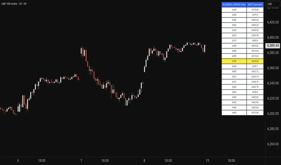
Pivot Points HL DetailedThis indicator marks important turning points in the market, showing you the most recent swing high and swing low as horizontal lines across the chart. Each pivot line has a price label where it formed and a small counter that updates whenever the market touches that level again. The line’s color reflects the prevailing trend, determined by an EMA filter, so you can quickly see if the level is likely acting as support or resistance in the current market environment.
It works by scanning recent bars for points where price made a local high higher than several bars to its left and right, or a local low lower than several bars to its left and right. These pivots are calculated directly from price action using the ta.pivothigh and ta.pivotlow functions. Once identified, the level is tracked in real time, counting every time price crosses it. The EMA provides context: if price is above the EMA, the market is considered in an uptrend and the pivots are colored to match; if price is below, they’re marked as part of a downtrend.
For traders, this offers a clean way to see where the market has turned before and whether those levels are still relevant. Strong levels often show multiple touches, which can be used for entries, exits, or risk management. The built-in alert system can notify you when price approaches either the most recent swing high or swing low, so you can react quickly.
This tool can be applied in almost any market — forex, stocks, indices, commodities, or crypto — because price tends to respect recent swing points regardless of the asset class. It tends to be most effective in liquid markets, where many traders see and react to the same key levels, and it’s valuable in both trending and ranging conditions, though the EMA trend filter adds extra clarity when the market is moving directionally.