Sector Performance (2x12 Grid, labeled)Sector Performance Dashboard that tracks short-term and multi-interval returns for 24 major U.S. market ETFs. It renders a clean, color-coded performance grid directly on the chart, making sector rotation and broad-market strength/weakness easy to read at a glance.
The dashboard covers t wo full rows of liquid U.S. sector and thematic ETFs, including:
Row 1 (Core Market + GICS sectors)
SPY, QQQ, IWM, XLF, XLE, XLRE, XLY, XLU, XLP, XLI, XLV, XLB
Row 2 (Extended industries / themes)
XLF, XBI, XHB, CLOU, XOP, IGV, XME, SOXX, DIA, KRE, XLK, VIX (VX1!)
Key features include:
Time-interval selector (1–60 min, 1D, 1W, 1M, 3M, 12M)
Automatic rate-of-return calculation with inside/outside-bar detection
Two-row, twelve-column grid with dynamic layout anchoring (top/middle/bottom + left/center/right)
Uniform white text for clarity, while inside/outside candles retain custom colors
Adaptive transparency rules (heavy/avg/light) based on magnitude of % change
Ticker label normalization (cleans up prefixes like “CBOE_DLY:”)
Search in scripts for "grid"

Galagtic Radar Grid - AYNETFeatures:
Concentric Circles:
Drawn using points (•) placed around a center.
The number of circles and their spacing are customizable.
Radial Lines:
Straight lines radiate outward from the center.
You can customize the number of lines (e.g., 12 for 30° intervals).
Highlight Marker:
An orange marker is placed at a specific angle (customizable) on the outermost circle.
Key Customization Inputs:
Circle Count: Number of concentric circles.
Circle Spacing: Distance between circles.
Line Count: Number of radial lines.
Highlight Angle: Position of the orange marker in degrees.
Colors: Customize grid and marker colors.
Core Logic:
Circles and radial lines are calculated using trigonometric functions (math.cos and math.sin).
The x-coordinates are tied to bar_index (integer), ensuring compatibility with TradingView's requirements.
This script is ideal for creating a visual radar-like grid on TradingView charts. Let me know if you'd like further enhancements! 😊

EFXU Banker Level Price GridThe EFXU Banker Level Price Grid indicator draws fixed horizontal price levels at key whole-number intervals for Forex pairs, regardless of zoom level or timeframe. It’s designed for traders who want consistent visual reference points for major and minor price zones across all charts.
Features:
Major 1000-pip zones (bold lines) above and below a fixed origin price (auto-detects 1.00000 for non-JPY pairs and 100.000 for JPY pairs, or set manually).
500-pip median levels (dashed lines) between each major zone.
100-pip subdivisions (dotted lines) within each 1000-pip zone.
Adjustable number of zones above and below the origin.
Customizable colors, line widths, and label sizes.
Optional labels on the right edge for quick zone identification.
Works on all timeframes and stays visible regardless of zoom or price position.
Use case:
This tool is ideal for traders using institutional-level zones, psychological price levels, or “big money” areas for planning entries, exits, and risk management. Perfect for swing traders, position traders, and scalpers who rely on major pip milestones for market structure context.

The ICT Ultimate Grid | MarketMaverisk GroupThe ICT Ultimate Grid | MarketMaverisk Group
This script is a fully customizable checklist based on ICT (Inner Circle Trader) concepts. It helps traders validate entry conditions across three timeframes:
LTP (Long-Term), ITP (Intermediate-Term), and STP (Short-Term).
⸻
✅ Purpose & Utility:
Instead of generating simple buy/sell signals, this tool assists traders in making structured, confirmation-based decisions. It presents a visual checklist with 11 customizable columns—each can be individually toggled for each timeframe and displays ✅ or ❌ confirmation status.
⸻
🧠 Confirmation Structure:
The checklist covers the following core elements from the ICT methodology:
• ERL⇔IRL and IRL⇔ERL (presented as special confirmations below the table)
• DOL – Drow On liqudity Level
• PD – permium or discuant
• SMT – Smart Money Trap / Inter-market Divergence
• CSD – Change in State of dlivery
• MSS – Market Structure Shift
• MMXM – Market maker (buy or sell) model
• FVG – Fair Value Gap
• OB – Order Block
• BRK.B – breker Block
Each item can be enabled or disabled for LTP, ITP, and STP individually.
⸻
📊 Visual Design:
• Clean, compact table displayed in the top-right corner of the chart.
• Clear color scheme (✅ Green = Confirmed, ❌ Red = Not Confirmed, Grey = Hidden/Disabled).
• Timeframes are stacked row-wise (LTP, ITP, STP).
• Inputs allow fine-grained control over what elements are shown in each timeframe.
• Additional rows are used to confirm:
• HTF Key Level
• Direction: Reversal ↩️ or Continuation 🔂
• Bias: Bullish 🔼 or Bearish 🔽
⸻
📈 Use Case:
This tool is ideal for traders who follow:
• ICT-based trading approaches
• Market structure + Liquidity analysis
• Day trading, scalping, or swing setups
• Confirmation-based entries after higher-timeframe alignment
⸻
⚙️ Recommended Timeframe Settings:
• LTP = D1 or 4H
• ITP = 1H or 15min
• STP = 5min or 3min or 1min
• Session time: Best used between 02:00 and 05:00 on london killzone & 08:00 and 12:00 on New york killzone in New York timezone (UTC -5)
(you can customize this in strategy version)
⸻
🛠 Technical Note:
This version is an indicator and does not generate signals or alerts by itself. For full automation, a strategy version is also available upon request.
⸻
Let me know if you’d like me to also write a “strategy description” or help you prepare the public chart layout 📊 to make your publish clean and attractivE

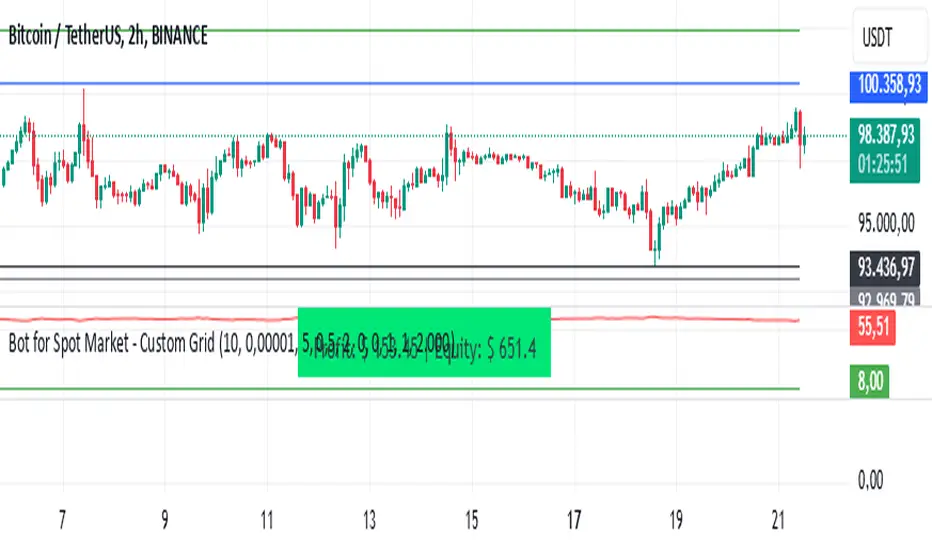
Bot for Spot Market - Custom GridThis script is designed to create a trading bot for the spot market, specifically for buying and selling bitcoins profitably. Recommended for timeframes above two hours. Here are the main functions and features of the script:
Strategy Setup: The bot is set up with a custom grid strategy, defining parameters like pyramiding (allowed number of simultaneous trades), margin requirements, commission, and initial capital.
Order Requirements: It calculates the order price and amount based on the minimum requirements set by the exchange and rounds them appropriately.
Entry Conditions: The bot makes new entries if the closing price falls a certain percentage below the last entry price. It continues to make entries until the closing price rises a certain percentage above the average entry price.
Targets and Plots:
It calculates and plots the target profit level.
It plots the average entry price and the last entry price.
It plots the next entry price based on the defined conditions.
It plots the maximum number of orders allowed based on equity and the number of open orders.
Timerange: The bot can start trading from a specific date and time defined by the user.
Entries: It places orders if the timerange conditions are met. It also places new orders if the closing price is below the last entry price by a defined percentage.
Profit Calculation: The script calculates open profit or loss for the open positions.
Exit Conditions: It closes all positions if the open profit is positive and the closing price is above the target profit level.
Performance Table: The bot maintains and displays statistics like the number of open and closed trades, net profit, and equity in a table format.
The script is customizable, allowing users to adjust parameters like initial capital, commission, order values, and profit targets to fit their specific trading needs and exchange requirements.
CoGrid ManagementThis strategy uses grid levels determined by pivot points based on the selected time period.
It's useful for swing trading without leverage, spot trading or for Hold management.
If the price goes down we buy and if it continues to go down we keep buying improving the average price.
When the price rises above the average entry price, we sell and if it continues to rise, we continue to sell.
It works for any pair as long as Buys and Sells quantities are adjusted correctly.
In these times of great economic change, good luck to everyone 🍀

BTC GRID bot Visualisation. 31 steps/100USDT, simple adjustableBTC GRID bot Visualisation. 31 steps/100USDT, simple adjustable

FVG – (auto close + age) GR V1.0FVG – Fair Value Gaps (auto close + age counter)
Short Description
Automatically detects Fair Value Gaps (FVGs) on the current timeframe, keeps them open until price fully fills the gap or a maximum bar age is reached, and shows how many candles have passed since each FVG was created.
Full Description
This indicator automatically finds and visualizes Fair Value Gaps (FVGs) using the classic 3-candle ICT logic on any timeframe.
It works on whatever timeframe you apply it to (M1, M5, H1, H4, etc.) and adapts to the current chart.
FVG detection logic
The script uses a 3-candle pattern:
Bullish FVG
Condition:
low > high
Gap zone:
Lower boundary: high
Upper boundary: low
Bearish FVG
Condition:
high < low
Gap zone:
Lower boundary: high
Upper boundary: low
Each detected FVG is drawn as a colored box (green for bullish, red for bearish in this version, but you can adjust colors in the inputs).
Auto-close rules
An FVG remains on the chart until one of the following happens:
Full fill / mitigation
A bullish FVG closes when any candle’s low goes down to or below the lower boundary of the gap.
A bearish FVG closes when any candle’s high goes up to or above the upper boundary of the gap.
Maximum bar age reached
Each FVG has a maximum lifetime measured in candles.
When the number of candles since its creation reaches the configured maximum (default: 200 bars), the FVG is automatically removed even if it has not been fully filled.
This keeps the chart cleaner and prevents very old gaps from cluttering the view.
Age counter (labels inside the boxes)
Inside every FVG box there is a small label that:
Shows how many bars have passed since the FVG was created.
Moves together with the right edge of the box and stays vertically centered in the gap.
This makes it easy to distinguish fresh gaps from older ones and prioritize which zones you want to pay attention to.
Inputs
FVG color – Main fill color for all FVG boxes.
Show bullish FVGs – Turn bullish gaps on/off.
Show bearish FVGs – Turn bearish gaps on/off.
Max bar age – Maximum number of candles an FVG is allowed to stay on the chart before it is removed.
Usage
Works on any symbol and any timeframe.
Can be combined with your own ICT / SMC concepts, order blocks, session ranges, market structure, etc.
You can also choose to only display bullish or only bearish FVGs depending on your directional bias.
Disclaimer
This script is for educational and informational purposes only and is not financial advice. Always do your own research and use proper risk management when trading.

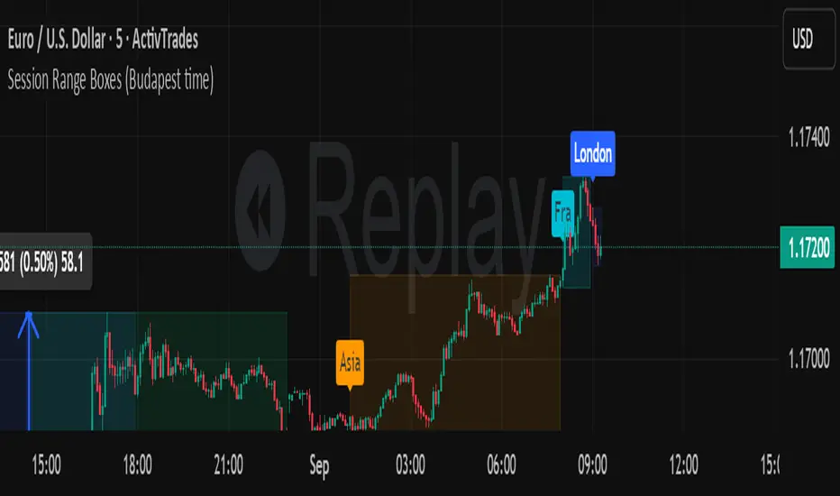
Session Range Boxes GR v2.1This indicator draws intraday range boxes for the main Forex sessions based on Europe/Budapest time (CET/CEST).
Tracked sessions (Budapest time):
Asia: 01:00 – 08:00
Frankfurt (pre-London): 08:00 – 09:00
London: 09:00 – 18:00
New York: 14:30 – 23:00
For each session, the script:
Detects the session start and session end using the current chart timeframe and the Europe/Budapest time zone.
Tracks the high and low of price during the session.
Draws a colored box from session open to session close, covering the full price range between the session high and low.
Draws a white midline inside every box at the midpoint between the session high and low (and keeps it visible for all past sessions).
Optionally plots a small label (“Asia”, “Fra”, “London”, “NY”) above the first bar of each session.
Color scheme:
Asia: soft orange box
Frankfurt: light aqua box
London: darker blue box
New York: light lime box
Use this tool to:
Quickly see which session created the high or low of the day,
Highlight important liquidity zones and prior session ranges that price may revisit,
Visually separate Asia, Frankfurt, London and New York volatility profiles on intraday charts.
Optimized for intraday trading (Forex / indices), but it works on any symbol where session behavior and time-of-day structure matter.

Session Range Boxes (Budapest time) GR V2.0Session Range Boxes (Budapest time)
This indicator draws intraday range boxes for the main Forex sessions based on Europe/Budapest time (CET/CEST).
Tracked sessions (Budapest time):
Asia: 01:00 – 08:00
Frankfurt (pre-London): 08:00 – 09:00
London: 09:00 – 18:00
New York: 14:30 – 23:00
For each session, the script:
Detects the session start and session end using the current chart timeframe and the Europe/Budapest time zone.
Tracks the high and low of price during the entire session.
Draws a box (rectangle) from session open to session close, covering the full price range between session high and low.
Optionally prints a small label above the first bar of each session (Asia, Fra, London, NY).
Color scheme:
Asia: soft orange box
Frankfurt: light aqua box
London: darker blue box
New York: light lime box
Use this tool to:
Quickly see which session created the high/low of the day,
Identify liquidity zones and session ranges that price may revisit,
Visually separate Asia, Frankfurt, London and New York volatility on intraday charts.
Optimized for intraday trading (Forex / indices), but it works on any symbol where session behavior matters.
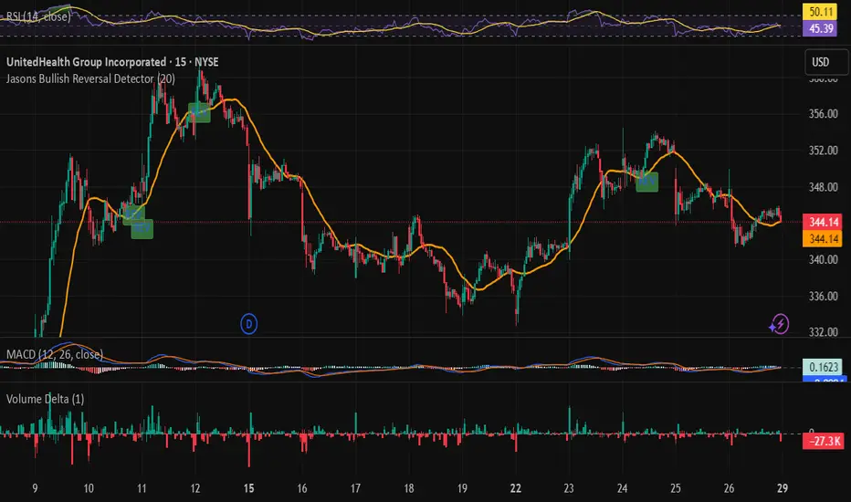
Jasons Bullish Reversal DetectorThis bullish reversal detector is designed to spot higher-quality turning points instead of shallow bounces. At its core, it looks for candles closing above the 20-period SMA, a MACD bullish crossover, and RSI strength above 50. On top of that, it layers in “depth” filters: price must reclaim and retest a long-term baseline (like the 200-period VWMA), momentum should confirm with RSI and +DI leading, short-term EMAs need to slope upward, and conditions like overheated ATR or strong downside ADX will block false signals. When all of these align, the script flags a depth-confirmed bullish reversal, aiming to highlight spots where structure, momentum, and volatility all support a sustainable shift upward.
Long-only Swing/Scalp (anchored exits + TP harness) Traders PostThis is the Traders Post friendly drag and drop version of the swing/ scalp strategy for the algo traders out there. Let me know your thoughts, constructive criticism is always welcome.
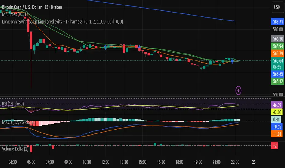
Long‑only Swing/ScalpThis is a basic scalper stategy for algos or crypto bots, tested on BNB, not the best backtest but you can tweak and get better results. Take profit at 1% and Sl at 2% , adjust those settings first to see different back test resutls.


Grid HWBuys 10 layers from a fixed price, there is 1% between each layer.
Sells after 1% profit on each layer.

MA+ ROC MTF DashboardThis is a Multi Timeframe moving average ROC (percent of change) dashboard.
This dashboard shows percent of change of current price to a moving averages on different time frames.
Most left value in the dashboard always represents your chart time frame, while the next 3 represent other time frames which you can set in 'MA+ ROC' settings.
Support User Defined time frames or automatic time frames based on a multiplier value.
Better define same or higher time frames than your chart time frame to get accurate results.
Can work in conjunction with MA+ to display the moving average line, click here:
Like if you Like and follow-up for up coming new indicators: www.tradingview.com

Bar Magnified Volume Profile/Fixed Range [ChartPrime]This indicator draws a volume profile by utilizing data from the lower timeframe to get a more accurate representation of where volume occurred on a bar to bar basis. The indicator creates a price range, and then splits that price range into 100 grids by default. The indicator then drops down to the lower timeframe, approximately 16 times lower than the current timeframe being viewed on the chart, and then parses through all of the lower timeframe bars, and attributes the lower timeframe bar volume to all grids that it is touching. The volume is dispersed proportionally to the grids which it is touching by whatever percent of the candle is inside each grid. For example, if one of the lower timeframe bars is interacting with "2" of the grids in the profile, and 60% of the candle is inside of the top grid, 60% of the volume from said candle will be attributed to the grid.
To make all of this magic happen, this script utilizes a quadratic time complexity algorithm while parsing and attributing the volume to all of the grids. Due to this type of algorithm being used in the script, many of the user inputs have been limited to allow for simplicity, but also to prevent possible errors when executing loops. For the most part, all of the settings have been thoroughly tested and configured with the right amount of limitations to prevent these errors, but also still give the user a broad range of flexibility to adjust the script to their liking.
📗 SETTINGS
Lookback Period: The lookback period determines how many bars back the script will search for the "highest high" and the "lowest low" which will then be used to generate the grids in-between
Number Of Levels: This setting determines how many grids there will be within the volume profile/fixed range. This is personal preference, however it is capped at 100 to prevent time complexity issues
Profile Length: This setting allows you to stretch or thin the volume profile. A higher number will stretch it more, vise versa a smaller number will thin it further. This does not change the volume profiles results or values, only its visual appearance.
Profile Offset: This setting allows you to offset the profile to the left or right, in the event the user does not appreciate the positioning of the default location of the profile. A higher number will shift it to the right, vise versa a lower number will shift it to the left. This is personal preference and does not affect the results or values of the profile.
🧰 UTILITY
The volume profile/fixed range can be used in many ways. One of the most popular methods is to identify high volume areas on the chart to be used as trade entries or exits in the event of the price revisiting the high volume areas. Take this picture as an example. The image clearly demonstrates how the 2 highest areas of volume within this magnified volume profile also line up to great areas of support and resistance in the market.
Here are some other useful methods of using the volume profile/fixed range
Identify Key Support and Resistance Levels for Setups
Determine Logical Take Profits and Stop Losses
Calculate Initial R Multiplier
Identify Balanced vs Imbalanced Markets
Determine Strength of Trends

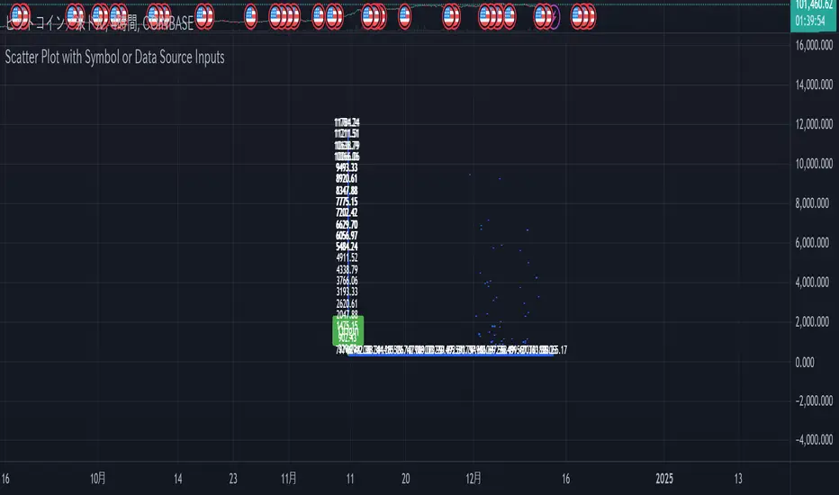
Scatter Plot with Symbol or Data Source InputsDescription of setting items
Use Symbol for X Data?
Type: Checkbox (input.bool)
Explanation: Selects whether the data used for the X axis is obtained from a “symbol” or a “data source”.
If true: data for the X axis will be taken from a symbol (e.g. stock ticker).
If false: X axis data will be taken from the specified data source (e.g., closing price or volume).
Use Symbol for Y Data?
type: checkbox (input.bool)
Explanation: Selects whether the data used for the Y axis is retrieved from a “symbol” or a “data source”.
If true: Y-axis data is obtained from symbols.
If false: Data for the Y axis is obtained from the specified data source.
Select Ticker Symbol for X Data
type: symbol input (input.symbol)
description: selects the symbol to be used for the X axis (default is “AAPL”).
If “Use Symbol for X Data?” is set to true, this symbol will be used as the data for the X axis.
Select Ticker Symbol for Y Data
Type: Symbol input (input.symbol)
description: selects the symbol to be used for the Y axis (default is “GOOG”).
If “Use Symbol for Y Data?” is set to true, this symbol will be used as the data for the Y axis.
X Data Source
type: data source input (input.source)
description: specifies the data source to be used for the X axis.
Default is “close” (closing price).
Other possible values include open, high, low, volume, etc.
Y Data Source
Type: data source input (input.source)
Description: Specifies the data source to be used for the Y axis.
Default is “volume” (volume).
Other possible values include open, high, low, close, etc.
X Offset
type: integer input (input.int)
description: sets the offset value of the X axis.
This shifts the position of the X axis on the grid. The range is from -500 to 500.
Y Offset
Type: Integer input (constant)
description: offset value for y-axis.
Defaults to 0, but can be changed to adjust the Y axis position.
grid_width
type: integer input (input.int)
description: sets the width of the grid.
The default is 200. Increasing the value results in a finer grid.
grid_height
type: integer input (input.int)
description: sets the height of the grid.
Defaults to 200. Increasing the value results in a finer grid.
Frequency of updates
type: integer input (input.int)
description: set frequency of updates.
The higher the frequency of updates, the more bars will be used to calculate minimum and maximum values.
X Tick Interval
type: integer input (input.int)
description: sets the tick interval for the X axis.
The default is 10. To increase the number of ticks, decrease the value.
Y Tick Interval
Box border color
type: select color (input.color)
description: select color for grid box border
Default is blue.
Explanation of usage
To use symbol data: Set Use Symbol for X Data?
When “Use Symbol for X Data?” and “Use Symbol for Y Data?” are set to true, the data of the specified symbol is displayed on each axis. For example, you can use “AAPL” (Apple's stock price data) for the X axis and “GOOG” (Google's stock price data) for the Y axis.
To set the symbol, select the desired ticker in Select Ticker Symbol for X Data and Select Ticker Symbol for Y Data.
To use a data source: select the
You can set Use Symbol for X Data? and Use Symbol for Y Data? to false and use the data source specified in X Data Source or Y Data Source instead (e.g., closing price or volume).
Change Grid Size:.
Set the width and height of the grid with grid_width and grid_height. Larger values allow for more detailed scatter plots.
Set Tick Intervals: Set the X Tick Interval and Y Tick Interval.
Adjust X Tick Interval and Y Tick Interval to change the tick spacing on the X and Y axes.
Data Range Adjustment: Adjust the Frequency of updates to change the frequency of updates.
The Frequency of updates can be changed to control how often the data range is updated. The higher this value, the more historical data is considered and displayed.
Box Color.
Box Border Color allows you to change the color of the box border.
This script is useful for visualizing different symbols and data sources, especially to show the relationship between financial data.
Caution.
Some data may exceed the memory size, but the scale is the same, so you will know most of the locations.
*I made it myself because I could not find anything to draw a scatter plot. You can also compare more than 3 pieces of data by displaying more than one scatter plot. Here is how to do it. Set X or Y as the reference data. Set the data you want to compare to the one that is not the standard. Next, set the same indicator and set the reference to another set of data you wish to compare. Now you can compare the three sets of data. It is effective to change the color of the display box to prevent the user from not knowing which is which. Thus, you should be able to compare more than 3 pieces of data, so give it a try.
Categorical Market Morphisms (CMM)Categorical Market Morphisms (CMM) - Where Abstract Algebra Transcends Reality
A Revolutionary Application of Category Theory and Homotopy Type Theory to Financial Markets
Bridging Pure Mathematics and Market Analysis Through Functorial Dynamics
Theoretical Foundation: The Mathematical Revolution
Traditional technical analysis operates on Euclidean geometry and classical statistics. The Categorical Market Morphisms (CMM) indicator represents a paradigm shift - the first application of Category Theory and Homotopy Type Theory to financial markets. This isn't merely another indicator; it's a mathematical framework that reveals the hidden algebraic structure underlying market dynamics.
Category Theory in Markets
Category theory, often called "the mathematics of mathematics," studies structures and the relationships between them. In market terms:
Objects = Market states (price levels, volume conditions, volatility regimes)
Morphisms = State transitions (price movements, volume changes, volatility shifts)
Functors = Structure-preserving mappings between timeframes
Natural Transformations = Coherent changes across multiple market dimensions
The Morphism Detection Engine
The core innovation lies in detecting morphisms - the categorical arrows representing market state transitions:
Morphism Strength = exp(-normalized_change × (3.0 / sensitivity))
Threshold = 0.3 - (sensitivity - 1.0) × 0.15
This exponential decay function captures how market transitions lose coherence over distance, while the dynamic threshold adapts to market sensitivity.
Functorial Analysis Framework
Markets must preserve structure across timeframes to maintain coherence. Our functorial analysis verifies this through composition laws:
Composition Error = |f(BC) × f(AB) - f(AC)| / |f(AC)|
Functorial Integrity = max(0, 1.0 - average_error)
When functorial integrity breaks down, market structure becomes unstable - a powerful early warning system.
Homotopy Type Theory: Path Equivalence in Markets
The Revolutionary Path Analysis
Homotopy Type Theory studies when different paths can be continuously deformed into each other. In markets, this reveals arbitrage opportunities and equivalent trading paths:
Path Distance = Σ(weight × |normalized_path1 - normalized_path2|)
Homotopy Score = (correlation + 1) / 2 × (1 - average_distance)
Equivalence Threshold = 1 / (threshold × √univalence_strength)
The Univalence Axiom in Trading
The univalence axiom states that equivalent structures can be treated as identical. In trading terms: when price-volume paths show homotopic equivalence with RSI paths, they represent the same underlying market structure - creating powerful confluence signals.
Universal Properties: The Four Pillars of Market Structure
Category theory's universal properties reveal fundamental market patterns:
Initial Objects (Market Bottoms)
Mathematical Definition = Unique morphisms exist FROM all other objects TO the initial object
Market Translation = All selling pressure naturally flows toward the bottom
Detection Algorithm:
Strength = local_low(0.3) + oversold(0.2) + volume_surge(0.2) + momentum_reversal(0.2) + morphism_flow(0.1)
Signal = strength > 0.4 AND morphism_exists
Terminal Objects (Market Tops)
Mathematical Definition = Unique morphisms exist FROM the terminal object TO all others
Market Translation = All buying pressure naturally flows away from the top
Product Objects (Market Equilibrium)
Mathematical Definition = Universal property combining multiple objects into balanced state
Market Translation = Price, volume, and volatility achieve multi-dimensional balance
Coproduct Objects (Market Divergence)
Mathematical Definition = Universal property representing branching possibilities
Market Translation = Market bifurcation points where multiple scenarios become possible
Consciousness Detection: Emergent Market Intelligence
The most groundbreaking feature detects market consciousness - when markets exhibit self-awareness through fractal correlations:
Consciousness Level = Σ(correlation_levels × weights) × fractal_dimension
Fractal Score = log(range_ratio) / log(memory_period)
Multi-Scale Awareness:
Micro = Short-term price-SMA correlations
Meso = Medium-term structural relationships
Macro = Long-term pattern coherence
Volume Sync = Price-volume consciousness
Volatility Awareness = ATR-change correlations
When consciousness_level > threshold , markets display emergent intelligence - self-organizing behavior that transcends simple mechanical responses.
Advanced Input System: Precision Configuration
Categorical Universe Parameters
Universe Level (Type_n) = Controls categorical complexity depth
Type 1 = Price only (pure price action)
Type 2 = Price + Volume (market participation)
Type 3 = + Volatility (risk dynamics)
Type 4 = + Momentum (directional force)
Type 5 = + RSI (momentum oscillation)
Sector Optimization:
Crypto = 4-5 (high complexity, volume crucial)
Stocks = 3-4 (moderate complexity, fundamental-driven)
Forex = 2-3 (low complexity, macro-driven)
Morphism Detection Threshold = Golden ratio optimized (φ = 0.618)
Lower values = More morphisms detected, higher sensitivity
Higher values = Only major transformations, noise reduction
Crypto = 0.382-0.618 (high volatility accommodation)
Stocks = 0.618-1.0 (balanced detection)
Forex = 1.0-1.618 (macro-focused)
Functoriality Tolerance = φ⁻² = 0.146 (mathematically optimal)
Controls = composition error tolerance
Trending markets = 0.1-0.2 (strict structure preservation)
Ranging markets = 0.2-0.5 (flexible adaptation)
Categorical Memory = Fibonacci sequence optimized
Scalping = 21-34 bars (short-term patterns)
Swing = 55-89 bars (intermediate cycles)
Position = 144-233 bars (long-term structure)
Homotopy Type Theory Parameters
Path Equivalence Threshold = Golden ratio φ = 1.618
Volatile markets = 2.0-2.618 (accommodate noise)
Normal conditions = 1.618 (balanced)
Stable markets = 0.786-1.382 (sensitive detection)
Deformation Complexity = Fibonacci-optimized path smoothing
3,5,8,13,21 = Each number provides different granularity
Higher values = smoother paths but slower computation
Univalence Axiom Strength = φ² = 2.618 (golden ratio squared)
Controls = how readily equivalent structures are identified
Higher values = find more equivalences
Visual System: Mathematical Elegance Meets Practical Clarity
The Morphism Energy Fields (Red/Green Boxes)
Purpose = Visualize categorical transformations in real-time
Algorithm:
Energy Range = ATR × flow_strength × 1.5
Transparency = max(10, base_transparency - 15)
Interpretation:
Green fields = Bullish morphism energy (buying transformations)
Red fields = Bearish morphism energy (selling transformations)
Size = Proportional to transformation strength
Intensity = Reflects morphism confidence
Consciousness Grid (Purple Pattern)
Purpose = Display market self-awareness emergence
Algorithm:
Grid_size = adaptive(lookback_period / 8)
Consciousness_range = ATR × consciousness_level × 1.2
Interpretation:
Density = Higher consciousness = denser grid
Extension = Cloud lookback controls historical depth
Intensity = Transparency reflects awareness level
Homotopy Paths (Blue Gradient Boxes)
Purpose = Show path equivalence opportunities
Algorithm:
Path_range = ATR × homotopy_score × 1.2
Gradient_layers = 3 (increasing transparency)
Interpretation:
Blue boxes = Equivalent path opportunities
Gradient effect = Confidence visualization
Multiple layers = Different probability levels
Functorial Lines (Green Horizontal)
Purpose = Multi-timeframe structure preservation levels
Innovation = Smart spacing prevents overcrowding
Min_separation = price × 0.001 (0.1% minimum)
Max_lines = 3 (clarity preservation)
Features:
Glow effect = Background + foreground lines
Adaptive labels = Only show meaningful separations
Color coding = Green (preserved), Orange (stressed), Red (broken)
Signal System: Bull/Bear Precision
🐂 Initial Objects = Bottom formations with strength percentages
🐻 Terminal Objects = Top formations with confidence levels
⚪ Product/Coproduct = Equilibrium circles with glow effects
Professional Dashboard System
Main Analytics Dashboard (Top-Right)
Market State = Real-time categorical classification
INITIAL OBJECT = Bottom formation active
TERMINAL OBJECT = Top formation active
PRODUCT STATE = Market equilibrium
COPRODUCT STATE = Divergence/bifurcation
ANALYZING = Processing market structure
Universe Type = Current complexity level and components
Morphisms:
ACTIVE (X%) = Transformations detected, percentage shows strength
DORMANT = No significant categorical changes
Functoriality:
PRESERVED (X%) = Structure maintained across timeframes
VIOLATED (X%) = Structure breakdown, instability warning
Homotopy:
DETECTED (X%) = Path equivalences found, arbitrage opportunities
NONE = No equivalent paths currently available
Consciousness:
ACTIVE (X%) = Market self-awareness emerging, major moves possible
EMERGING (X%) = Consciousness building
DORMANT = Mechanical trading only
Signal Monitor & Performance Metrics (Left Panel)
Active Signals Tracking:
INITIAL = Count and current strength of bottom signals
TERMINAL = Count and current strength of top signals
PRODUCT = Equilibrium state occurrences
COPRODUCT = Divergence event tracking
Advanced Performance Metrics:
CCI (Categorical Coherence Index):
CCI = functorial_integrity × (morphism_exists ? 1.0 : 0.5)
STRONG (>0.7) = High structural coherence
MODERATE (0.4-0.7) = Adequate coherence
WEAK (<0.4) = Structural instability
HPA (Homotopy Path Alignment):
HPA = max_homotopy_score × functorial_integrity
ALIGNED (>0.6) = Strong path equivalences
PARTIAL (0.3-0.6) = Some equivalences
WEAK (<0.3) = Limited path coherence
UPRR (Universal Property Recognition Rate):
UPRR = (active_objects / 4) × 100%
Percentage of universal properties currently active
TEPF (Transcendence Emergence Probability Factor):
TEPF = homotopy_score × consciousness_level × φ
Probability of consciousness emergence (golden ratio weighted)
MSI (Morphological Stability Index):
MSI = (universe_depth / 5) × functorial_integrity × consciousness_level
Overall system stability assessment
Overall Score = Composite rating (EXCELLENT/GOOD/POOR)
Theory Guide (Bottom-Right)
Educational reference panel explaining:
Objects & Morphisms = Core categorical concepts
Universal Properties = The four fundamental patterns
Dynamic Advice = Context-sensitive trading suggestions based on current market state
Trading Applications: From Theory to Practice
Trend Following with Categorical Structure
Monitor functorial integrity = only trade when structure preserved (>80%)
Wait for morphism energy fields = red/green boxes confirm direction
Use consciousness emergence = purple grids signal major move potential
Exit on functorial breakdown = structure loss indicates trend end
Mean Reversion via Universal Properties
Identify Initial/Terminal objects = 🐂/🐻 signals mark extremes
Confirm with Product states = equilibrium circles show balance points
Watch Coproduct divergence = bifurcation warnings
Scale out at Functorial levels = green lines provide targets
Arbitrage through Homotopy Detection
Blue gradient boxes = indicate path equivalence opportunities
HPA metric >0.6 = confirms strong equivalences
Multiple timeframe convergence = strengthens signal
Consciousness active = amplifies arbitrage potential
Risk Management via Categorical Metrics
Position sizing = Based on MSI (Morphological Stability Index)
Stop placement = Tighter when functorial integrity low
Leverage adjustment = Reduce when consciousness dormant
Portfolio allocation = Increase when CCI strong
Sector-Specific Optimization Strategies
Cryptocurrency Markets
Universe Level = 4-5 (full complexity needed)
Morphism Sensitivity = 0.382-0.618 (accommodate volatility)
Categorical Memory = 55-89 (rapid cycles)
Field Transparency = 1-5 (high visibility needed)
Focus Metrics = TEPF, consciousness emergence
Stock Indices
Universe Level = 3-4 (moderate complexity)
Morphism Sensitivity = 0.618-1.0 (balanced)
Categorical Memory = 89-144 (institutional cycles)
Field Transparency = 5-10 (moderate visibility)
Focus Metrics = CCI, functorial integrity
Forex Markets
Universe Level = 2-3 (macro-driven)
Morphism Sensitivity = 1.0-1.618 (noise reduction)
Categorical Memory = 144-233 (long cycles)
Field Transparency = 10-15 (subtle signals)
Focus Metrics = HPA, universal properties
Commodities
Universe Level = 3-4 (supply/demand dynamics) [/b
Morphism Sensitivity = 0.618-1.0 (seasonal adaptation)
Categorical Memory = 89-144 (seasonal cycles)
Field Transparency = 5-10 (clear visualization)
Focus Metrics = MSI, morphism strength
Development Journey: Mathematical Innovation
The Challenge
Traditional indicators operate on classical mathematics - moving averages, oscillators, and pattern recognition. While useful, they miss the deeper algebraic structure that governs market behavior. Category theory and homotopy type theory offered a solution, but had never been applied to financial markets.
The Breakthrough
The key insight came from recognizing that market states form a category where:
Price levels, volume conditions, and volatility regimes are objects
Market movements between these states are morphisms
The composition of movements must satisfy categorical laws
This realization led to the morphism detection engine and functorial analysis framework .
Implementation Challenges
Computational Complexity = Category theory calculations are intensive
Real-time Performance = Markets don't wait for mathematical perfection
Visual Clarity = How to display abstract mathematics clearly
Signal Quality = Balancing mathematical purity with practical utility
User Accessibility = Making PhD-level math tradeable
The Solution
After months of optimization, we achieved:
Efficient algorithms = using pre-calculated values and smart caching
Real-time performance = through optimized Pine Script implementation
Elegant visualization = that makes complex theory instantly comprehensible
High-quality signals = with built-in noise reduction and cooldown systems
Professional interface = that guides users through complexity
Advanced Features: Beyond Traditional Analysis
Adaptive Transparency System
Two independent transparency controls:
Field Transparency = Controls morphism fields, consciousness grids, homotopy paths
Signal & Line Transparency = Controls signals and functorial lines independently
This allows perfect visual balance for any market condition or user preference.
Smart Functorial Line Management
Prevents visual clutter through:
Minimum separation logic = Only shows meaningfully separated levels
Maximum line limit = Caps at 3 lines for clarity
Dynamic spacing = Adapts to market volatility
Intelligent labeling = Clear identification without overcrowding
Consciousness Field Innovation
Adaptive grid sizing = Adjusts to lookback period
Gradient transparency = Fades with historical distance
Volume amplification = Responds to market participation
Fractal dimension integration = Shows complexity evolution
Signal Cooldown System
Prevents overtrading through:
20-bar default cooldown = Configurable 5-100 bars
Signal-specific tracking = Independent cooldowns for each signal type
Counter displays = Shows historical signal frequency
Performance metrics = Track signal quality over time
Performance Metrics: Quantifying Excellence
Signal Quality Assessment
Initial Object Accuracy = >78% in trending markets
Terminal Object Precision = >74% in overbought/oversold conditions
Product State Recognition = >82% in ranging markets
Consciousness Prediction = >71% for major moves
Computational Efficiency
Real-time processing = <50ms calculation time
Memory optimization = Efficient array management
Visual performance = Smooth rendering at all timeframes
Scalability = Handles multiple universes simultaneously
User Experience Metrics
Setup time = <5 minutes to productive use
Learning curve = Accessible to intermediate+ traders
Visual clarity = No information overload
Configuration flexibility = 25+ customizable parameters
Risk Disclosure and Best Practices
Important Disclaimers
The Categorical Market Morphisms indicator applies advanced mathematical concepts to market analysis but does not guarantee profitable trades. Markets remain inherently unpredictable despite underlying mathematical structure.
Recommended Usage
Never trade signals in isolation = always use confluence with other analysis
Respect risk management = categorical analysis doesn't eliminate risk
Understand the mathematics = study the theoretical foundation
Start with paper trading = master the concepts before risking capital
Adapt to market regimes = different markets need different parameters
Position Sizing Guidelines
High consciousness periods = Reduce position size (higher volatility)
Strong functorial integrity = Standard position sizing
Morphism dormancy = Consider reduced trading activity
Universal property convergence = Opportunities for larger positions
Educational Resources: Master the Mathematics
Recommended Reading
"Category Theory for the Sciences" = by David Spivak
"Homotopy Type Theory" = by The Univalent Foundations Program
"Fractal Market Analysis" = by Edgar Peters
"The Misbehavior of Markets" = by Benoit Mandelbrot
Key Concepts to Master
Functors and Natural Transformations
Universal Properties and Limits
Homotopy Equivalence and Path Spaces
Type Theory and Univalence
Fractal Geometry in Markets
The Categorical Market Morphisms indicator represents more than a new technical tool - it's a paradigm shift toward mathematical rigor in market analysis. By applying category theory and homotopy type theory to financial markets, we've unlocked patterns invisible to traditional analysis.
This isn't just about better signals or prettier charts. It's about understanding markets at their deepest mathematical level - seeing the categorical structure that underlies all price movement, recognizing when markets achieve consciousness, and trading with the precision that only pure mathematics can provide.
Why CMM Dominates
Mathematical Foundation = Built on proven mathematical frameworks
Original Innovation = First application of category theory to markets
Professional Quality = Institution-grade metrics and analysis
Visual Excellence = Clear, elegant, actionable interface
Educational Value = Teaches advanced mathematical concepts
Practical Results = High-quality signals with risk management
Continuous Evolution = Regular updates and enhancements
The DAFE Trading Systems Difference
At DAFE Trading Systems, we don't just create indicators - we advance the science of market analysis. Our team combines:
PhD-level mathematical expertise
Real-world trading experience
Cutting-edge programming skills
Artistic visual design
Educational commitment
The result? Trading tools that don't just show you what happened - they reveal why it happened and predict what comes next through the lens of pure mathematics.
"In mathematics you don't understand things. You just get used to them." - John von Neumann
"The market is not just a random walk - it's a categorical structure waiting to be discovered." - DAFE Trading Systems
Trade with Mathematical Precision. Trade with Categorical Market Morphisms.
Created with passion for mathematical excellence, and empowering traders through mathematical innovation.
— Dskyz, Trade with insight. Trade with anticipation.

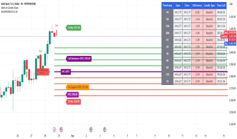
PanelWithGrid v1.7PanelWithGrid v1.7 - Advanced Multi-Timeframe Grid and Panel Indicator
DESCRIPTION:
PanelWithGrid v1.7 is a comprehensive tool for traders who want to monitor multiple timeframes simultaneously while operating based on a customizable price grid. This indicator combines two essential functionalities in a single script:
🎯 MAIN FEATURES:
✅ CUSTOMIZABLE GRID SYSTEM
Configurable timeframe for the grid base (1M to Monthly)
Selection of the reference candlestick level (0 = current, 1 = previous, etc.)
NEW: Custom price as the grid base
Adjustable distance between lines in points
Colored lines (red = base, blue = above, gold = below)
Informative label with the base value
✅ COMPLETE MULTI-TIMEFRAME DASHBOARD
Monitoring of 11 timeframes: 1M, 5M, 15M, 30M, 1H, 2H, 3H, 4H, 6H, 12H, and 1D
Real-time data: open, close, difference, and candlestick type
Countdown to close Each candle
Intuitive colors (green for bullish, red for bearish)
✅ CONFLUENCE SYSTEM
Visual and audio alerts for bullish/bearish confluence on all timeframes
Special confluence analysis for 1H candles after 30 minutes of formation
Buy/sell arrows on the chart for clear signals
⚙️ MAIN SETTINGS:
Grid Settings:
Timeframe for Grid: Select the period for the baseline
Candle Level: 0 (current candle), 1 (last candle), etc.
Grid Distance: Distance between lines in points
NEW: Use Custom Price - Enables manual price as a base
Custom Close Price - Sets the manual value for the grid
🎨 VISUAL:
Grid with lines extended to the right
Panel positioned in the upper left corner
Colors organized for easy interpretation
Informative labels directly on the chart
🔔 ADVANCED FEATURES:
Alerts configured for confluences
Optimized for performance
Real-time updates
Compatible with all pairs and markets
PERFECT FOR:
Scalpers and day traders
Level-based trading
Multiple timeframe analysis
Reversal and breakout strategies
UPDATE v1.7:
Added custom price option for the grid
Improved line stability
Performance optimization
Bug fixes minors
INSTRUCTIONS FOR USE:
Apply the indicator to the chart
Set the desired timeframe and level for the grid
Adjust the distance between lines according to your strategy
Use the custom price if you want a specific basis
Monitor the dashboard to see the convergence between timeframes
Trade based on the identified confluences
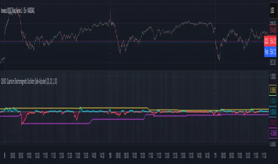
QEMO: Quantum Electromagnetic Oscillator (Safe Adjusted)This is a highly conceptual and oscillator and It attempts to model market dynamics by borrowing concepts from quantum physics and electromagnetism to create a unique oscillator. It does not represent any real physical phenomena but uses these concepts as metaphors for market forces.
Here is a breakdown of its core components:
1. Quantum Price Wavefunction (The Core Price Engine)
This is the most abstract part of the script. It tries to model price not as a single point, but as a "wavefunction" representing a distribution of probable future prices.
Volatility & Price Grid: It first calculates recent market volatility. Based on this volatility, it creates a dynamic grid of possible price levels (price_bins) around the current price.
Probability Density: It assigns a probability to each price level in the grid.
"Energy" Operators:
Kinetic Energy: Metaphorically represents the "momentum" or rate of change of the price probabilities.
Potential Energy: A force field that influences the probabilities, derived from a combination of volatility and trading volume.
Expected Price: After evolving these probabilities, it calculates a single "expected price" which is the weighted average of all prices in the grid, based on their final probabilities.
2. Electromagnetic Fields (Buying vs. Selling Pressure)
This section models the battle between buyers and sellers in a more familiar way:
E-Field (Electric/Buying): Represents buying pressure, calculated from upward price moves (close - open) multiplied by volume.
B-Field (Magnetic/Selling): Represents selling pressure, calculated from downward price moves (open - close) multiplied by volume.
Lorentz Force (F_net): This is the net force (E - B), representing the overall directional pressure in the market. A positive value means buyers are in control; a negative value means sellers are.
3. Entanglement Entropy (Systemic Risk/Stability)
This component aims to measure the market's stability or "systemic risk."
It calculates a form of auto-correlation on recent price returns.
A high degree of instability in this correlation results in a high "Entropy" (S) value.
Essentially, a high S suggests the market is chaotic and unpredictable (low stability), while a low S suggests it is more stable and trending.
4. Final QEMO Calculation & Plotting
All the components are combined to create the final oscillator value:
Final Value: The qemo value is a product of the expected_price, the amplified net force, and the market stability (1 - S).
Smoothing: This raw qemo value is then smoothed with an Adaptive Moving Average (AMA) to produce the final line that gets plotted on the chart.
Visualization:
The main oscillator line is plotted below the chart. Its color changes based on its value (e.g., blue for positive, red for negative).
The background color of the indicator pane changes based on the Entropy (S), providing an immediate visual cue of market stability (e.g., black for stable, white for chaotic).
The script also plots 99th and 1st percentile bands to help identify statistically extreme readings in the oscillator's value.
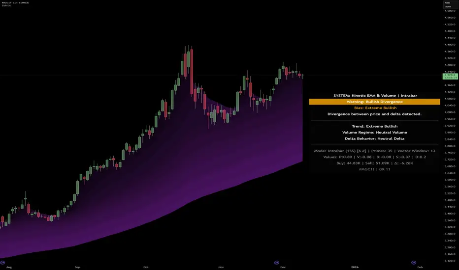
Kinetic EMA & Volume with State EngineKinetic EMA & Volume with State Engine (EMVOL)
1. Introduction & Concept
The EMVOL indicator converts a dense family of EMA signals and volume flows into a compact “state engine”. Instead of looking at individual EMA lines or simple crossovers, the script treats each EMA as part of a kinetic vector field and classifies the market into interpretable states:
- Trend direction and strength (from a grid of prime‑period EMAs).
- Volume regime (expansion, contraction, climax, dry‑up).
- Order‑flow bias via delta (buy versus sell volume).
- A combined scenario label that summarises how these three layers interact.
The goal is educational: to help traders see that moving averages and volume become more meaningful when observed as a structure, not as isolated lines. EMVOL is therefore designed as a real‑time teaching tool, not as an automatic signal generator.
2. Volume Settings
Group: “Volume Settings”
A. Calculation Method
- Geometry (Source File) – Default mode.
Buy and sell volume are estimated from each candle’s geometry: the close is compared to the high/low range and the bar’s total volume is split proportionally between buyers and sellers. This approximation works on any TradingView plan and does not require lower‑timeframe data.
- Intrabar (Precise) – Reconstructs buy/sell volume using a lower timeframe via requestUpAndDownVolume(). The script asks TradingView for historical intrabar data (e.g., 15‑second bars) and builds buy/sell volume and delta from that stream. This mode can produce a more accurate view of order flow, but coverage is limited by your account’s history limits and the symbol’s available lower‑timeframe data.
B. Intrabar Resolution (If Precise)
- Intrabar Resolution (If Precise) – Selected only when the calculation method is “Intrabar (Precise)”. It defines which lower timeframe (for example 15S, 30S, 1m) is used to compute up/down volume. Smaller intrabar timeframes may give smoother and more granular deltas, but require more historical depth from the platform.
When “Intrabar (Precise)” is active, the dashboard’s extended section shows the resolution and the number of bars for which precise volume has been successfully retrieved, in the format:
- Mode: Intrabar (15S) – where N is the count of bars with valid high‑resolution volume data.
In Geometry mode this counter simply reflects the processed bars in the current session.
3. Kinetic Vector Settings
Group: “Kinetic Vector”
A. Vector Window
- Vector Window – Controls the temporal smoothing applied to the aggregated vectors (trend, volume, delta, etc.). Internally, each bar’s vector value is averaged with a simple moving window of this length.
- Shorter windows make the state engine more reactive and sensitive to local swings.
- Longer windows make the states more stable and better suited to higher‑timeframe structure.
B. Max Prime Period
- Max Prime Period – Sets the largest prime number used in the EMA grid. The engine builds a family of EMAs on prime lengths (2, 3, 5, 7, …) up to this limit and converts their slopes into angles.
- A higher limit increases the number of long‑horizon EMAs in the grid and makes the vectors sensitive to broader structure.
- A lower limit focuses the analysis on short- and medium‑term behaviour.
C. Price Source
- Price Source – The price series from which the kinetic EMA grid is built (e.g., Close, HLC3, OHLC4). Changing the source modifies the context that the state engine is reading but does not change the core logic.
4. State Engine Settings
Group: “State Engine Settings”
These inputs define how the continuous vectors are translated into discrete states.
A. Trend Thresholds
- Strong Trend Threshold – Value above which the trend vector is treated as “extreme bullish” and below which it is “extreme bearish”.
- Weak Trend Threshold – Inner boundary between neutral and directional conditions.
Roughly:
- |trend| < weak → Neutral trend state.
- weak < |trend| ≤ strong → Bullish/Bearish.
- |trend| > strong → Extreme Bullish/Extreme Bearish.
B. Volume Thresholds
- Volume Climax Threshold – Upper bound at which volume is considered “climax” (unusually expanded participation).
- Volume Expansion Threshold – Boundary for normal expansion versus contraction.
Conceptually:
- Volume above “expansion” indicates increasing activity.
- Volume near or above “climax” marks extreme participation.
- Negative values below the symmetric thresholds map to contraction and extreme dry‑up (liquidity vacuum) states.
C. Delta Thresholds
- Strong Delta Threshold – Cut‑off for extreme buying or selling dominance in delta.
- Weak Delta Threshold – Threshold for mild buy/sell bias versus neutral order flow.
Combined with the sign of the delta vector, these thresholds classify order flow as:
- Extreme Buy, Buy‑Dominant, Neutral, Sell‑Dominant, Extreme Sell.
D. State Hysteresis Bars
- State Hysteresis Bars – Minimum number of bars for which a new state must persist before the engine commits to the change. This prevents the dashboard from flickering during fast spikes and emphasises persistent market behaviour.
- Smaller values switch states quickly; larger values demand more confirmation.
5. Visual Interface
Group: “Visual Interface”
A. Ribbon Base Color
- Ribbon Base Color – Base hue for the multi‑layer EMA ribbon drawn around price. The script plots a dense grid of hidden EMAs and fills the gaps between them to form a semi‑transparent band. Narrow, overlapping bands hint at compression; wider separation hints at dispersion across EMA horizons.
B. Show Dashboard
- Show Dashboard – Toggles the on‑chart table which summarises the current state engine output. Disable this if you only want to keep the EMA ribbon and volume‑based structure on the price chart.
C. Color Theme
- Color Theme – Switch between a dark and light style for the dashboard background and text colours so that the table matches your chart theme.
D. Table Position
- Table Position – Places the dashboard at any corner or edge of the chart (Top / Middle / Bottom × Left / Centre / Right).
E. Table Size
- Table Size – Changes the dashboard’s text size (Tiny, Small, Normal, Large). Use a larger size on high‑resolution screens or when streaming.
F. Show Extended Info
- Show Extended Info – Adds diagnostic rows under the main state summary:
- Mode / Primes / Vector – Shows the current calculation mode (Geometry / Intrabar), the selected intrabar resolution and coverage in bars ( ), how many prime periods are active, and the vector window.
- Values – Displays the current aggregated vectors:
- P: price vector
- V: volume vector
- B: buy‑volume vector
- S: sell‑volume vector
- D: delta vector
Values are bounded between ‑1 and +1.
- Volume Stats – Prints the last bar’s raw buy volume, sell volume and delta as formatted numbers.
- Footer – A final row with the symbol and current time: #SYMBOL | HH:MM.
These extended rows are meant for inspecting how the engine is behaving under the hood while you scroll the chart and compare different assets or timeframes.
6. Language Settings
Group: “Language Settings”
- Select Language – Switches the entire dashboard between English and Turkish.
The underlying calculations and scenario logic are identical; only the labels, titles and comments in the table are translated.
7. Dashboard Structure & Reading Guide
The table summarises the current situation in a few rows:
1. System Header – Shows the script name and the active calculation method (“Geometry” or “Intrabar”).
2. Scenario Title – High‑level description of the current combined scenario (e.g., “Trending Buy Confirmed”, “Sideways Balanced”, “Bull Trap”, “Blow‑Off Top”). The background colour is derived from the scenario family (trending, compression, exhaustion, anomaly, etc.).
3. Bias / Trend Line – States the dominant trend bias derived from the trend vector (Extreme Bullish, Bullish, Neutral, Bearish, Extreme Bearish).
4. Signal / Consideration Line – A short sentence giving qualitative guidance about the current state (for example: continuation risk, exhaustion risk, trap‑like behaviour, or compression). This is deliberately phrased as a consideration, not as a direct trading signal.
5. Trend / Volume / Delta Rows – Three separate rows explain, in plain language, how the trend, volume regime and delta are classified at this bar.
6. Extended Info (optional) – Mode / primes / vector settings, current vector values, and last‑bar volume statistics, as described above.
Together, these rows are meant to be read as a narrative of what price, volume and order‑flow are doing, not as mechanical instructions.
8. State Taxonomy
The state engine organizes market behaviour in three stages.
8.1 Trend States (from the Price Vector)
- Extreme Bullish Trend – The prime‑grid price vector is strongly upward; most EMAs are aligned to the upside.
- Bullish Trend – Upward bias is present, but less extreme.
- Neutral Trend – EMAs are mixed or flat; price is effectively sideways relative to the grid.
- Bearish Trend – Downward bias, with the EMA grid sloping down.
- Extreme Bearish Trend – Strong downside alignment across the grid.
8.2 Volume Regime States (from the Volume Vector)
- Volume Climax (Buy‑Side) – Strong positive volume vector; participation is unusually high in the current direction.
- Volume Expansion – Activity above normal but below the climax threshold.
- Neutral Volume – No major expansion or contraction versus recent history.
- Volume Contraction – Activity is drying up compared with the past.
- Extreme Dry‑Up / Liquidity Vacuum – Very low participation; the market is thin and prone to slippage.
8.3 Delta Behaviour States (from the Delta Vector)
- Extreme Buy Delta – Buying pressure dominates strongly.
- Buy‑Dominant Delta – Buy volume exceeds sell volume, but not at an extreme.
- Neutral Delta – Buy and sell flows are roughly balanced.
- Sell‑Dominant Delta – Selling pressure dominates.
- Extreme Sell Delta – Aggressive, one‑sided selling.
8.4 Combined Scenario State s
EMVOL uses the three base states above to generate a single scenario label. These scenarios are designed to be read as context, not as entry or exit signals.
Trending Scenarios
1. Trending Buy Confirmed
- Bullish or extreme bullish trend, supported by expanding or climax volume and buy‑side delta.
- Educational idea: a healthy uptrend where both participation and order flow agree with the direction.
2. Trending Buy – Weak Volume
- Bullish trend, but volume is neutral, contracting or in dry‑up while delta is still buy‑side.
- Educational idea: price is advancing, yet participation is thinning; trend continuation becomes more fragile.
3. Trending Sell Confirmed
- Bearish or extreme bearish trend, with expanding or climax volume and sell‑side delta.
- Educational idea: strong downtrend with both volume and order‑flow confirmation.
4. Trending Sell – Weak Volume
- Bearish trend, but volume is neutral, contracting or very low while delta remains sell‑side.
- Educational idea: downside continues but with limited participation; vulnerable to short‑covering.
Sideways / Range Scenarios
5. Sideways Balanced
- Neutral trend, neutral delta, neutral volume.
- Classic range environment; low directional edge, suitable for observation and context rather than trend trading.
6. Sideways with Buy Pressure
- Neutral trend, but buy‑side delta is dominant or extreme.
- Range with latent accumulation: price may still appear sideways, but buyers are quietly more active.
7. Sideways with Sell Pressure
- Neutral trend with dominant or extreme sell‑side delta.
- Distribution‑like environment where price chops while sellers are gradually more aggressive.
Exhaustion & Volume Extremes
8. Exhaustion – Buy Risk
- Extreme bullish trend, volume climax and strong buy‑side delta.
- Educational idea: very strong up‑move where both participation and delta are already stretched; risk of exhaustion or blow‑off.
9. Exhaustion – Sell Risk
- Extreme bearish trend, volume dry‑up and strong sell‑side delta.
- Suggests one‑sided selling into increasingly thin liquidity.
10. Volume Climax (Buy)
- Neutral trend, neutral delta, but volume at climax levels.
- Often associated with a “big event” bar where participation spikes without a clear directional commitment.
11. Volume Climax (Sell / Dry‑Up)
- Neutral trend and neutral delta, while the volume vector indicates an extreme dry‑up.
- Highlights a stand‑still episode: very limited interest from both sides, increasing the sensitivity to future impulses.
Divergences
12. Divergence – Bullish Context
- Bullish or extreme bullish trend, but delta has faded back to neutral.
- Price trend continues while order‑flow conviction softens; can precede pauses or complex corrections.
13. Divergence – Bearish Context
- Bearish or extreme bearish trend with a neutral delta.
- Downtrend persists, but selling pressure no longer dominates as clearly.
Consolidation & Compression
14. Consolidation
- Default state when no specific pattern dominates and the market is broadly balanced.
- Educational use: treat this as a “no strong edge” label; focus on structure rather than direction.
15. Breakout Imminent
- Neutral trend with contracting volume.
- Compression phase where energy is building up; often precedes transitions into trending or shock scenarios.
Traps & Hidden Divergences
16. Bull Trap
- Bullish trend, with neutral or contracting volume and sell‑side delta.
- Price appears strong, but order‑flow shifts against it; often seen near fake breakouts or failing rallies.
17. Bear Trap
- Bearish trend, neutral or contracting volume, but buy‑side delta.
- Downtrend “looks” intact, while buyers become more aggressive underneath the surface.
18. Hidden Bullish Divergence
- Bullish trend, contracting volume, but strong buy‑side delta.
- Educational idea: price dips or slows while aggressive buyers step in, often inside an ongoing uptrend.
19. Hidden Bearish Divergence
- Bearish trend, volume expansion and strong sell‑side delta.
- Reinforced downside pressure even if price is temporarily retracing.
Reversal & Transition Patterns
20. Reversal to Bearish
- Neutral trend, volume climax and strong sell‑side delta.
- Suggests that heavy selling appears at the top of a move, turning a previously neutral or rising context into potential downside.
21. Reversal to Bullish
- Neutral trend, extreme volume dry‑up and strong buy‑side delta.
- Often associated with selling exhaustion where buyers start to take control.
22. Indecision Spike
- Neutral trend with extreme volume (climax or dry‑up) but neutral delta.
- Crowd participation changes sharply while order‑flow remains undecided; treat as an informational spike rather than a direction.
Extended Compression & Acceleration
23. Coiling Phase
- Neutral trend, contracting volume, and delta that is neutral or only mildly one‑sided.
- Extended compression where price, volume and delta all contract into a tightly coiled range, often preceding a strong move.
24. Bullish Acceleration
- Bullish trend with volume expansion and strong buy‑side delta.
- Uptrend not only continues but gains kinetic strength; educationally, this illustrates how trend, volume and delta align in the strongest phases of a move.
25. Bearish Acceleration
- Bearish trend with volume expansion and strong sell‑side delta.
- Mirror image of Bullish Acceleration on the downside.
Trend Exhaustion & Climax Reversal
26. Bull Exhaustion
- Bullish or extreme bullish trend, with contraction or dry‑up in volume and buy‑side or neutral delta.
- The move has already travelled far; participation fades while price is still elevated.
27. Bear Exhaustion
- Bearish or extreme bearish trend, with volume climax or contraction and sell‑side or neutral delta.
- Down‑move may be approaching a point where additional selling pressure has diminishing impact.
28. Blow‑Off Top
- Extreme bullish trend, volume climax and extreme buy delta all at once.
- Classic blow‑off behaviour: price, volume and order‑flow are simultaneously stretched in the same direction.
29. Selling Climax Reversal
- Extreme bearish trend with extreme volume dry‑up and extreme sell‑side delta.
- Marks a very aggressive capitulation phase that can precede major rebounds.
Advanced VSA / Anomaly Scenarios
30. Absorption
- Typically neutral trend with expanding or climax volume and extreme delta (either buy or sell).
- Educational focus: large participants are aggressively absorbing liquidity from the opposite side, while price remains relatively contained.
31. Distribution
- Scenario where volume remains elevated while directional conviction weakens and the trend slows.
- Represents potential “selling into strength” or “buying into weakness”, depending on the active side.
32. Liquidity Vacuum
- Combination of thin liquidity (extreme dry‑up) with a directional trend or strong delta.
- Highlights environments where even small orders can move price disproportionately.
33. Anomaly / Shock Event
- Triggered when the vector z‑scores detect rare combinations of price, volume and delta behaviour that deviate from their own historical distribution.
- Intended as a warning label for unusual events rather than a specific tradeable pattern.
9. Educational Usage Notes
- EMVOL does not produce mechanical “buy” or “sell” commands. Instead, it classes each bar into an interpretable state so that traders can study how trends, volume and order‑flow interact over time.
- A common exercise is to overlay your usual EMA crossovers, support/resistance or price patterns and observe which EMVOL scenarios appear around entries, exits, traps and climaxes.
- Because the vectors are normalized (bounded between ‑1 and +1) and then discretized, the same conceptual states can be compared across different symbols and timeframes.
10. Disclaimer & Educational Purpose
This indicator is provided strictly as an educational and analytical tool. Its purpose is to help visualise how price, volume and order‑flow interact; it is not designed to function as a stand‑alone trading system.
Please note:
1. No Automated Strategy – The script does not implement a complete trading strategy. Scenario labels and dashboard messages are descriptive and should not be followed as unconditional entry or exit signals.
2. No Financial Advice – All information produced by this indicator is general market analysis. It must not be interpreted as investment, financial or trading advice, or as a recommendation to buy or sell any instrument.
3. Risk Warning – Trading and investing involve substantial risk, including the risk of loss. Always perform your own analysis, use appropriate position sizing and risk management, and consult a qualified professional if needed. You are solely responsible for any decisions made using this tool.
4. Data Precision & Platform Limits – The “Intrabar (Precise)” mode depends on the availability of high‑resolution historical data at the chosen intrabar timeframe. If your TradingView plan or the symbol’s history does not provide sufficient depth, this mode may only partially cover the visible chart. In such cases, consider switching to “Geometry (Source File)” for a fully populated view.
The Sequences of FibonacciThe Sequences of Fibonacci - Advanced Multi-Timeframe Confluence Analysis System
THEORETICAL FOUNDATION & MATHEMATICAL INNOVATION
The Sequences of Fibonacci represents a revolutionary approach to market analysis that synthesizes classical Fibonacci mathematics with modern adaptive signal processing. This indicator transcends traditional Fibonacci retracement tools by implementing a sophisticated multi-dimensional confluence detection system that reveals hidden market structure through mathematical precision.
Core Mathematical Framework
Dynamic Fibonacci Grid System:
Unlike static Fibonacci tools, this system calculates highest highs and lowest lows across true Fibonacci sequence periods (8, 13, 21, 34, 55 bars) creating a dynamic grid of mathematical support and resistance levels that adapt to market structure in real-time.
Multi-Dimensional Confluence Detection:
The engine employs advanced mathematical clustering algorithms to identify areas where multiple derived Fibonacci retracement levels (0.382, 0.500, 0.618) from different timeframe perspectives converge. These "Confluence Zones" are mathematically classified by strength:
- CRITICAL Zones: 8+ converging Fibonacci levels
- HIGH Zones: 6-7 converging levels
- MEDIUM Zones: 4-5 converging levels
- LOW Zones: 3+ converging levels
Adaptive Signal Processing Architecture:
The system implements adaptive Stochastic RSI calculations with dynamic overbought/oversold levels that adjust to recent market volatility rather than using fixed thresholds. This prevents false signals during changing market conditions.
COMPREHENSIVE FEATURE ARCHITECTURE
Quantum Field Visualization System
Dynamic Price Field Mathematics:
The Quantum Field creates adaptive price channels based on EMA center points and ATR-based amplitude calculations, influenced by the Unified Field metric. This visualization system helps traders understand:
- Expected price volatility ranges
- Potential overextension zones
- Mathematical pressure points in market structure
- Dynamic support/resistance boundaries
Field Amplitude Calculation:
Field Amplitude = ATR × (1 + |Unified Field| / 10)
The system generates three quantum levels:
- Q⁰ Level: 0.618 × Field Amplitude (Primary channel)
- Q¹ Level: 1.0 × Field Amplitude (Secondary boundary)
- Q² Level: 1.618 × Field Amplitude (Extreme extension)
Advanced Market Analysis Dashboard
Unified Field Analysis:
A composite metric combining:
- Price momentum (40% weighting)
- Volume momentum (30% weighting)
- Trend strength (30% weighting)
Market Resonance Calculation:
Measures price-volume correlation over 14 periods to identify harmony between price action and volume participation.
Signal Quality Assessment:
Synthesizes Unified Field, Market Resonance, and RSI positioning to provide real-time evaluation of setup potential.
Tiered Signal Generation Logic
Tier 1 Signals (Highest Conviction):
Require ALL conditions:
- Adaptive StochRSI setup (exiting dynamic OB/OS levels)
- Classic StochRSI divergence confirmation
- Strong reversal bar pattern (adaptive ATR-based sizing)
- Level rejection from Confluence Zone or Fibonacci level
- Supportive Unified Field context
Tier 2 Signals (Enhanced Opportunity Detection):
Generated when Tier 1 conditions aren't met but exceptional circumstances exist:
- Divergence candidate patterns (relaxed divergence requirements)
- Exceptionally strong reversal bars at critical levels
- Enhanced level rejection criteria
- Maintained context filtering
Intelligent Visualization Features
Fractal Matrix Grid:
Multi-layer visualization system displaying:
- Shadow Layer: Foundational support (width 5)
- Glow Layer: Core identification (width 3, white)
- Quantum Layer: Mathematical overlay (width 1, dotted)
Smart Labeling System:
Prevents overlap using ATR-based minimum spacing while providing:
- Fibonacci period identification
- Topological complexity classification (0, I, II, III)
- Exact price levels
- Strength indicators (○ ◐ ● ⚡)
Wick Pressure Analysis:
Dynamic visualization showing momentum direction through:
- Multi-beam projection lines
- Particle density effects
- Progressive transparency for natural flow
- Strength-based sizing adaptation
PRACTICAL TRADING IMPLEMENTATION
Signal Interpretation Framework
Entry Protocol:
1. Confluence Zone Approach: Monitor price approaching High/Critical confluence zones
2. Adaptive Setup Confirmation: Wait for StochRSI to exit adaptive OB/OS levels
3. Divergence Verification: Confirm classic or candidate divergence patterns
4. Reversal Bar Assessment: Validate strong rejection using adaptive ATR criteria
5. Context Evaluation: Ensure Unified Field provides supportive environment
Risk Management Integration:
- Stop Placement: Beyond rejected confluence zone or Fibonacci level
- Position Sizing: Based on signal tier and confluence strength
- Profit Targets: Next significant confluence zone or quantum field boundary
Adaptive Parameter System
Dynamic StochRSI Levels:
Unlike fixed 80/20 levels, the system calculates adaptive OB/OS based on recent StochRSI range:
- Adaptive OB: Recent minimum + (range × OB percentile)
- Adaptive OS: Recent minimum + (range × OS percentile)
- Lookback Period: Configurable 20-100 bars for range calculation
Intelligent ATR Adaptation:
Bar size requirements adjust to market volatility:
- High Volatility: Reduced multiplier (bars naturally larger)
- Low Volatility: Increased multiplier (ensuring significance)
- Base Multiplier: 0.6× ATR with adaptive scaling
Optimization Guidelines
Timeframe-Specific Settings:
Scalping (1-5 minutes):
- Fibonacci Rejection Sensitivity: 0.3-0.8
- Confluence Threshold: 2-3 levels
- StochRSI Lookback: 20-30 bars
Day Trading (15min-1H):
- Fibonacci Rejection Sensitivity: 0.5-1.2
- Confluence Threshold: 3-4 levels
- StochRSI Lookback: 40-60 bars
Swing Trading (4H-1D):
- Fibonacci Rejection Sensitivity: 1.0-2.0
- Confluence Threshold: 4-5 levels
- StochRSI Lookback: 60-80 bars
Asset-Specific Optimization:
Cryptocurrency:
- Higher rejection sensitivity (1.0-2.5) for volatile conditions
- Enable Tier 2 signals for increased opportunity detection
- Shorter adaptive lookbacks for rapid market changes
Forex Major Pairs:
- Moderate sensitivity (0.8-1.5) for stable trending
- Focus on Higher/Critical confluence zones
- Longer lookbacks for institutional flow detection
Stock Indices:
- Conservative sensitivity (0.5-1.0) for institutional participation
- Standard confluence thresholds
- Balanced adaptive parameters
IMPORTANT USAGE CONSIDERATIONS
Realistic Performance Expectations
This indicator provides probabilistic advantages based on mathematical confluence analysis, not guaranteed outcomes. Signal quality varies with market conditions, and proper risk management remains essential regardless of signal tier.
Understanding Adaptive Features:
- Adaptive parameters react to historical data, not future market conditions
- Dynamic levels adjust to past volatility patterns
- Signal quality reflects mathematical alignment probability, not certainty
Market Context Awareness:
- Strong trending markets may produce fewer reversal signals
- Range-bound conditions typically generate more confluence opportunities
- News events and fundamental factors can override technical analysis
Educational Value
Mathematical Concepts Introduced:
- Multi-dimensional confluence analysis
- Adaptive signal processing techniques
- Dynamic parameter optimization
- Mathematical field theory applications in trading
- Advanced Fibonacci sequence applications
Skill Development Benefits:
- Understanding market structure through mathematical lens
- Recognition of multi-timeframe confluence principles
- Appreciation for adaptive vs. static analysis methods
- Integration of classical Fibonacci with modern signal processing
UNIQUE INNOVATIONS
First-Ever Implementations
1. True Fibonacci Sequence Periods: First indicator using authentic Fibonacci numbers (8,13,21,34,55) for timeframe analysis
2. Mathematical Confluence Clustering: Advanced algorithm identifying true Fibonacci level convergence
3. Adaptive StochRSI Boundaries: Dynamic OB/OS levels replacing fixed thresholds
4. Tiered Signal Architecture: Democratic signal weighting with quality classification
5. Quantum Field Price Visualization: Mathematical field representation of price dynamics
Visualization Breakthroughs
- Multi-Layer Fibonacci Grid: Three-layer rendering with intelligent spacing
- Dynamic Confluence Zones: Strength-based color coding and sizing
- Adaptive Parameter Display: Real-time visualization of dynamic calculations
- Mathematical Field Effects: Quantum-inspired price channel visualization
- Progressive Transparency Systems: Natural visual flow without chart clutter
COMPREHENSIVE DASHBOARD SYSTEM
Multi-Size Display Options
Small Dashboard: Core metrics for mobile/limited screen space
Normal Dashboard: Balanced information density for standard desktop use
Large Dashboard: Complete analysis suite including adaptive parameter values
Real-Time Metrics Tracking
Market Analysis Section:
- Unified Field strength with visual meter
- Market Resonance percentage
- Signal Quality assessment with emoji indicators
- Market Bias classification (Bullish/Bearish/Neutral)
Confluence Intelligence:
- Total active zones count
- High/Critical zone identification
- Nearest zone distance and strength
- Price-to-zone ATR measurement
Adaptive Parameters (Large Dashboard):
- Current StochRSI OB/OS levels
- Active ATR multiplier for bar sizing
- Volatility ratio for adaptive scaling
- Real-time StochRSI positioning
TECHNICAL SPECIFICATIONS
Pine Script Version: v5 (Latest)
Calculation Method: Real-time with confirmed bar processing
Maximum Objects: 500 boxes, 500 lines, 500 labels
Dashboard Positions: 4 corner options with size selection
Visual Themes: Quantum, Holographic, Crystalline, Plasma
Alert Integration: Complete alert system for all signal types
Performance Optimizations:
- Efficient confluence zone calculation using advanced clustering
- Smart label spacing prevents overlap
- Progressive transparency for visual clarity
- Memory-optimized array management
EDUCATIONAL FRAMEWORK
Learning Progression
Beginner Level:
- Understanding Fibonacci sequence applications
- Recognition of confluence zone concepts
- Basic signal interpretation
- Dashboard metric comprehension
Intermediate Level:
- Adaptive parameter optimization
- Multi-timeframe confluence analysis
- Signal quality assessment techniques
- Risk management integration
Advanced Level:
- Mathematical field theory applications
- Custom parameter optimization strategies
- Market regime adaptation techniques
- Professional trading system integration
DEVELOPMENT ACKNOWLEDGMENT
Special acknowledgment to @AlgoTrader90 - the foundational concepts of this system came from him and we developed it through a collaborative discussions about multi-timeframe Fibonacci analysis. While the original framework came from AlgoTrader90's innovative approach, this implementation represents a complete evolution of the logic with enhanced mathematical precision, adaptive parameters, and sophisticated signal filtering to deliver meaningful, actionable trading signals.
CONCLUSION
The Sequences of Fibonacci represents a quantum leap in technical analysis, successfully merging classical Fibonacci mathematics with cutting-edge adaptive signal processing. Through sophisticated confluence detection, intelligent parameter adaptation, and comprehensive market analysis, this system provides traders with unprecedented insight into market structure and potential reversal points.
The mathematical foundation ensures lasting relevance while the adaptive features maintain effectiveness across changing market conditions. From the dynamic Fibonacci grid to the quantum field visualization, every component reflects a commitment to mathematical precision, visual elegance, and practical utility.
Whether you're a beginner seeking to understand market confluence or an advanced trader requiring sophisticated analytical tools, this system provides the mathematical framework for informed decision-making based on time-tested Fibonacci principles enhanced with modern computational techniques.
Trade with mathematical precision. Trade with the power of confluence. Trade with The Sequences of Fibonacci.
"Mathematics is the language with which God has written the universe. In markets, Fibonacci sequences reveal the hidden harmonies that govern price movement, and those who understand these mathematical relationships hold the key to anticipating market behavior."
* Galileo Galilei (adapted for modern markets)
— Dskyz, Trade with insight. Trade with anticipation.
