Gann Square of Nine: Planetary Degrees█ Gann Square of Nine: Planetary Degrees maps planetary positions onto Gann's Square of Nine grid, tracking where pivot highs and lows accumulate by planetary degree. Use this indicator to identify recurring degree patterns on the So9, determine whether pivots cluster around cardinal, diagonal, or other significant angles, and project when the planet will return to those degrees.
Powered by the open-source BlueprintResearch Planetary Ephemeris library , which implements truncated VSOP87 (planets) and ELP2000 (Moon) series for high-accuracy celestial calculations entirely within Pine Script.
█ FEATURES
• Anchor Point System — Select any significant price pivot (high or low) as your reference point; all subsequent pivot tracking begins from this timestamp
• All 10 celestial bodies — Sun, Moon, Mercury, Venus, Mars, Jupiter, Saturn, Uranus, Neptune, and Pluto
• Geocentric or Heliocentric views — Toggle between Earth-centered (traditional) and Sun-centered perspectives
• Interactive Square of Nine table — Visual grid displaying the Gann spiral pattern with highlighted pivot degrees
• Automatic pivot detection — Configurable bar sensitivity to identify price pivots (symmetric left/right)
• Pivot degree labeling — Each detected pivot displays the planet's ecliptic longitude (0-360°) at that moment
• Target degree alerts — Define specific So9 degrees to watch; triggers alerts when the planet crosses them
• Preset So9 angles — Quick selection of degrees along major So9 lines (0°, 45°, 90°, 135°, 180°, 225°, 270°, 315°)
• Custom degree input — Enter any degrees as comma-separated or newline-separated values
• Future degree projections — Scans up to 500 bars ahead and shows when the planet will reach each target degree
• Retrograde indicator — Shows ℞ symbol with red text when planets are in apparent retrograde motion
• So9 overlay tools — Plot 90° and 45° angle relationships from any entered degree
█ HOW IT WORKS
The Square of Nine Concept:
Gann's Square of Nine is a spiral grid where numbers flow outward from the center (1) in a square spiral pattern. Key angle relationships (0°, 45°, 90°, etc.) align along specific diagonals and cardinal lines. When planetary degrees land on the same So9 position as significant price pivots, it suggests potential support/resistance levels.
This Indicator:
1. User selects an "anchor" timestamp at a significant price pivot
2. The indicator calculates the selected planet's ecliptic longitude (0-360°) at each bar
3. Price pivots detected after the anchor are labeled with their planetary degrees
4. These degrees accumulate on the So9 grid, revealing patterns
5. Target degrees can be set to receive alerts when crossed
6. Future projections show when the planet will reach those target degrees
█ HOW TO USE
1. Click on the anchor timestamp input and select a significant high or low pivot on your chart
2. Choose "High" or "Low" pivot type based on your anchor point
3. Select your planet from the dropdown
4. Choose Geocentric (traditional) or Heliocentric view
5. The So9 table appears showing accumulated pivot degrees highlighted
6. Set target degrees using presets or custom input to receive crossing alerts
7. Future projections appear as vertical lines with date/time labels
8. Use the So9 overlay tools to visualize angle relationships from specific degrees
█ VISUAL GUIDE
So9 Table Colors:
• Anchor degree: White (⚓ symbol)
• Current planet position: Planet's assigned color with symbol
• Pivot Highs: Green background
• Pivot Lows: Red background
• Equal (both high and low): Orange background
• Diagonal crosses: Blue background
• Cardinal crosses: Red background
• Target degrees: Yellow highlight
Chart Labels:
• Pivot High labels appear above the price with the degree
• Pivot Low labels appear below the price with the degree
• Future projection lines: Yellow (upcoming) or Gray (already crossed since anchor)
█ SETTINGS OVERVIEW
1. Anchor Point — Set the starting pivot timestamp and type (High/Low)
2. Planet Selection — Choose celestial body and coordinate system
3. Target Degree Alerts — Configure which degrees to watch and receive alerts
4. Pivot Detection — Set bar sensitivity for pivot high/low detection and degree rounding precision
5. Visual Style — Customize colors and label sizes
6. So9 Grid Overlay — Enter a degree to visualize its angular relationships
7. So9 Table — Position, sizing, and color options for the grid
8. So9 Diagonals — Toggle and color the diagonal/cardinal cross highlights
█ LIMITATIONS & ACCURACY
This indicator uses optimized VSOP87 and ELP2000 series tailored for Pine Script performance. It delivers excellent accuracy for trading and analytical purposes.
Expected Accuracy:
• Sun, Moon, Mercury, Venus, Mars: Within 1-10 arcseconds
• Jupiter, Saturn: Within 10-30 arcseconds
• Uranus, Neptune: Within 1-2 arcminutes
• Pluto: Simplified Meeus method (valid 1900-2100)
Degree Resolution:
The So9 grid uses integer degrees (1-361). Planetary positions are rounded to the nearest whole degree for grid placement. Precise decimal degrees are retained for crossing calculations and alerts.
Crossing Detection:
Future projection lines and background highlights both point to the confirmation bar—the first bar where the crossing can be verified. Alerts also trigger on this bar. This ensures all visual elements align consistently: when the chart reaches a future projection line, that bar closes with the crossing confirmed and highlighted.
█ CREDITS
• Square of Nine grid visualization adapted from ThiagoSchmitz's "Gann Square of 9" (Feb 2023)
• Ephemeris calculations via BlueprintResearch/lib_ephemeris open-source library
Search in scripts for "grid"

nATR*ATR Multiplication Indicator - Optimal Selection Tool forThis indicator is specifically designed as an analysis tool for investors using grid bot strategies. It displays both nATR (Normalized Average True Range) and ATR (Average True Range) values on a single chart screen, calculating the multiplication of these two critical volatility measurements.
Primary Purpose of the Indicator:
To facilitate the selection of the most optimal stock and time period for grid bot trading. The nATR*ATR multiplication provides a hybrid measurement that combines both percentage-based return potential (nATR) and absolute volatility magnitude (ATR).
Importance for Grid Bot Strategy:
High nATR: Greater percentage-based return potential
High ATR: Wider price range = Fewer grid levels = More budget allocation per grid
Formula: Price Range/ATR = Theoretical Grid Count
Usage Advantages:
Test different time periods to find the highest multiplication value
Make optimal stock and time frame selections for grid bot setup
Monitor both nATR and ATR values on a single screen
High multiplication values indicate ideal conditions for grid bots
Technical Features:
Adjustable calculation period (1-500 candles)
Visual alert system (high/low multiplication values)
Real-time value tracking table
SMA-based smoothed calculations
This serves as a reliable guide for grid bot investors in optimal timing and stock selection.

CE - 42MACRO Fixed Income and Macro This is Part 2 of 2 from the 42MACRO Recreation Series
However, there will be a bonus Indicator coming soon!
The CE - 42MACRO Fixed Income and Macro Table is a next level Macroeconomic and market analysis indicator.
It aims to provide a probabilistic insight into the market realized GRID Macro regimes,
track a multiplex of important Assets, Indices, Bonds and ETF's to derive extra market insights by showing the most important aggregates and their performance over multiple timeframes... and what that might mean for the whole market direction.
For traders and especially investors, the unique functionalities will be of high value.
Quick guide on how to use it:
docs.google.com
WARNING
By the nature of the macro regimes, the outcomes are more accurate over longer Chart Timeframes (Week to Months).
However, it is also a valuable tool to form an advanced,
market realized, short to medium term bias.
NOTE
This Indicator is intended to be used alongside the 1nd part "CE - 42MACRO Equity Factor"
for a more wholistic approach and higher accuracy.
Methodology:
The Equity Factor Table tracks specifically chosen Assets to identify their performance and add the combined performances together to visualize 42MACRO's GRID Equity Model.
For this it uses the below Assets:
Convertibles ( AMEX:CWB )
Leveraged Loans ( AMEX:BKLN )
High Yield Credit ( AMEX:HYG )
Preferreds ( NASDAQ:PFF )
Emerging Market US$ Bonds ( NASDAQ:EMB )
Long Bond ( NASDAQ:TLT )
5-10yr Treasurys ( NASDAQ:IEF )
5-10yr TIPS ( AMEX:TIP )
0-5yr TIPS ( AMEX:STIP )
EM Local Currency Bonds ( AMEX:EMLC )
BDCs ( AMEX:BIZD )
Barclays Agg ( AMEX:AGG )
Investment Grade Credit ( AMEX:LQD )
MBS ( NASDAQ:MBB )
1-3yr Treasurys ( NASDAQ:SHY )
Bitcoin ( AMEX:BITO )
Industrial Metals ( AMEX:DBB )
Commodities ( AMEX:DBC )
Gold ( AMEX:GLD )
Equity Volatility ( AMEX:VIXM )
Interest Rate Volatility ( AMEX:PFIX )
Energy ( AMEX:USO )
Precious Metals ( AMEX:DBP )
Agriculture ( AMEX:DBA )
US Dollar ( AMEX:UUP )
Inverse US Dollar ( AMEX:UDN )
Functionalities:
Fixed Income and Macro Table
Shows relative market Asset performance
Comes with different Calculation options like RoC,
Sharpe ratio, Sortino ratio, Omega ratio and Normalization
Allows for advanced market (health) performance
Provides the calculated, realized GRID market regimes
Informs about "Risk ON" and "Risk OFF" market states
Visuals - for your best experience only use one (+ BarColoring) at a time:
You can visualize all important metrics:
- GRID regimes of the currently chosen calculation type
- Risk On/Risk Off with background colouring and additional +1/-1 values
- a smoother GRID model
- a smoother Risk On/ Risk Off metric
- Barcoloring for enabled metric of the above
If you have more suggestions, please write me
Fixed Income and Macro:
The visualisation of the relative performance of the different assets provides valuable information about the current market environment and the actual market performance.
It furthermore makes it possible to obtain a deeper understanding of how the interconnected market works and makes it simple to identify the actual market direction,
thus also providing all the information to derive overall market health, market strength or weakness.
Utility:
The Fixed Income and Macro Table is divided in 4 Columns which are the GRID regimes:
Economic Growth:
Goldilocks
Reflation
Economic Contraction:
Inflation
Deflation
Top 5 Fixed Income/ Macro Factors:
Are the values green for a specific Column?
If so then the market reflects the corresponding GRID behavior.
Bottom 5 Fixed Income/ Macro Factors:
Are the values red for a specific Column?
If so then the market reflects the corresponding GRID behavior.
So if we have Goldilocks as current regime we would see green values in the Top 5 Goldilocks Cells and red values in the Bottom 5 Goldilocks Cells.
You will find that Reflation will look similar, as it is also a sign of Economic Growth.
Same is the case for the two Contraction regimes.
******
This Indicator again is based to a majority on 42MACRO's models.
I only brought them into TV and added things on top of it.
If you have questions or need a more in-depth guide DM me.
GM

Psychological levels [Kodologic] Psychological levels
Markets are not random, they are driven by human psychology and algorithmic order flow. A well-known phenomenon in trading is the "Whole Number Bias" — the tendency for price to react significantly at clean, round numbers (e.g., Bitcoin at $95,000 or EURUSD at 1.0500).
Manually drawing horizontal lines at every round number is tedious, clutters your object tree, and distracts you from analyzing price action.
Psychological levels Numbers is a workflow utility designed to solve this problem. It automatically projects a clean, customizable grid of key price levels onto your chart, helping you instantly identify areas where liquidity and orders are likely to cluster.
Why This Indicator Helps Traders :
Professional traders know that "00" and "50" levels act as magnets for price. Here is how this tool assists in your analysis:
1. Institutional Footprints : Large institutions and bank algorithms often execute orders at whole numbers to simplify accounting. This script highlights these potential liquidity zones automatically.
2. Support & Resistance Discovery: You will often notice price wicking or reversing exactly on these grid lines. This helps in spotting natural support and resistance without needing complex technical analysis.
3. Cognitive Load Reduction: Instead of calculating where the next "major level" is, the grid is visually present, allowing you to focus on candlestick patterns and market structure.
Features :
Dynamic Calculation : The grid updates automatically as price moves, you never have to redraw lines.
Zero Clutter : The lines are drawn using code, meaning they do not appear in your manual drawing tools list or clutter your object tree.
Fully Customizable Step : You define what constitutes a "Round Number" for your specific asset class (Forex, Crypto, Indices, or Stocks).
Visual Control : Adjust line styles (Solid, Dotted, Dashed), colors, and transparency to keep your chart aesthetic and readable.
How to Use in Your Strategy :
1. Target Setting (Take Profit)
If you are in a long position, use the next upper grid line as a logical Take Profit area. Price often gravitates toward these whole numbers before reversing or consolidating.
2. Stop Loss Placement
Avoid placing Stop Losses exactly on a round number, as these are often "stop hunted." Instead, use the grid to visualize the level and place your stop slightly *below* or *above* the round number for better protection.
3. Confluence Trading
Do not use these lines in isolation. Look for Confluence :
Example: If a Fibonacci 61.8% level lines up exactly with a Round Number grid line, that level becomes a high-probability reversal zone.
Settings Guide (Important)
Since every asset is priced differently, you must adjust the "levels Step Size" to match your instrument:
Forex (e.g., EURUSD, GBPUSD): Set Step Size to `0.0050` (50 pips) or `0.0100` (100 pips).
Crypto (e.g., BTCUSD): Set Step Size to `500` or `1000`.
Indices (e.g., US30, SPX500): Set Step Size to `100` or `500`.
Gold (XAUUSD):** Set Step Size to `10`.
Disclaimer: This tool is for educational and visual aid purposes only. It does not provide buy or sell signals. Always manage your risk.

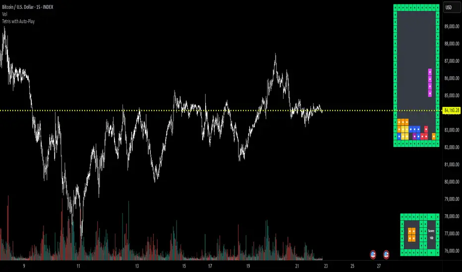
Tetris with Auto-PlayThis indicator is implemented in Pine Script™ v6 and serves as a demonstration of TradingView's capabilities. The core concept is to simulate a classic Tetris game by creating a grid-based environment and managing game state entirely within Pine Script.
Key Technical Aspects:
Grid Representation:
The script defines a custom grid structure using a user-defined type that holds the grid’s dimensions and a one-dimensional array to simulate a two-dimensional board. This structure is used to track occupied cells, clear full rows, and determine stack height.
Piece Management:
A second custom type is used to represent the state of a tetromino piece, including its type, rotation, and position. The code includes functions to calculate the block offsets for each tetromino based on its rotation state.
Collision Detection and Piece Locking:
Dedicated functions check for collisions against the grid borders and existing blocks. When a collision is detected during a downward move, the piece is locked into the grid, and any complete lines are cleared.
AIgo-Driven Placement:
The script incorporates a simple heuristic to determine the best placement for the next tetromino. It simulates different rotations and horizontal positions, evaluating each based on aggregated column height, cleared lines, holes, and bumpiness. This decision-making process is encapsulated in an AI-like function that returns the optimal rotation and placement.
Rendering Using Tables:
The visual representation is managed via TradingView’s table objects. The game board is rendered with a bordered layout, while a separate preview table displays the next piece and the current score. Each cell is updated with text and background colors that correspond to the state of the game.
Execution Flow and Timing:
The main execution loop handles real-time updates by dropping pieces at set intervals and checking for game-over conditions. The code leverages persistent variables and time comparisons to control game speed and manage transitions between piece drops.
Executing:
Add the indicator to the chart
It starts playing itself till game over
There are no parameters to change in this version but the grid in the code directly
p.s. Sadly we have no interactive buttons in the current pinescript versions to play ourself, but its about the possibilitys what we could do ;-)
Maybe in a future version there is more possible, if i find time to enhance and expand the idea
Have fun :-)
CE - 42MACRO Equity Factor Table This is Part 1 of 2 from the 42MACRO Recreation Series
The CE - 42MACRO Equity Factor Table is a whole toolbox packaged in a single indicator.
It aims to provide a probabilistic insight into the market realized GRID Macro Regime, use a multiplex of important Assets and Indices to form a high probability Implied Correlation expectation and allows to derive extra market insights by showing the most important aggregates and their performance over multiple timeframes... and what that might mean for the whole market direction, as well as the underlying asset.
WARNING
By the nature of the macro regimes, the outcomes are more accurate over longer Chart Timeframes (Week to Months).
However, it is also a valuable tool to form a proper,
market realized, short to medium term bias.
NOTE
This Indicator is intended to be used alongside the 2nd part "CE - 42MACRO Yield and Macro"
for a more wholistic approach and higher accuracy.
Due to coding limitations they can not be merged into one Indicator.
Methodology:
The Equity Factor Table tracks specifically chosen Assets to identify their performance and add the combined performances together to visualize 42MACRO's GRID Equity Model.
For this it uses the below Assets, with more to come:
Dividend Compounders ( AMEX:SPHD )
Mid Caps ( AMEX:VO )
Emerging Markets ( AMEX:EEM )
Small Caps ( AMEX:IWM )
Mega Cap Growth ( NASDAQ:QQQ )
Brazil ( AMEX:EWZ )
United Kingdom ( AMEX:EWU )
Growth ( AMEX:IWF )
United States ( AMEX:SPY )
Japan ( AMEX:DXJ )
Momentum ( AMEX:MTUM )
China ( AMEX:FXI )
Low Beta ( AMEX:SPLV )
International ex-US ( NASDAQ:ACWX )
India ( AMEX:INDA )
Eurozone ( AMEX:EZU )
Quality ( AMEX:QUAL )
Size ( AMEX:OEF )
Functionalities:
1. Correlations
Takes a measure of Cross Market Correlations
2. Implied Trend
Calculates the trend for each Asset and uses the Correlation to obtain the Implied Trend for the underlying Asset
There are multiple functionalities to enhance Signal Speed and precision...
Reading a signal only over a certain threshold, otherwise being colored in gray to signal noise or unclear market behavior
Normalization of Signal
Double Normalization of Signal for more Speed... ideal for the Crypto Market
Using an additional Hull Moving Average to enhance Signal Speed
Additional simple Background coloring to get a Signal from the HMA
Barcoloring based on the Implied Correlation
3. Equity Factor Table
Shows market realized Asset performance
Provides the approximate realized GRID market regimes
Informs about "Risk ON" and "Risk OFF" market states
Now into the juicy stuff...
Visuals:
There is a variety of options to change visual settings of what is plotted and where
+ additional considerations.
Everything that is relevant in the underlying logic which can improve comprehension can be visualized with these options.
More to come
Market Correlation:
The Market Correlation Table takes the Correlation of all the Assets to the Asset on the Chart,
it furthermore uses the Normalized KAMA Oscillator by IkkeOmar to analyse the current trend of every single Asset.
(To enhance the Signal you can apply the mentioned Indicator on the relevant Assets to find your target Asset movements that you intend to capture...
and then change the length of the Indicator in here)
It then Implies a Correlation based on the Trend and the Correlation to give a probabilistically adjusted expectation for the future Chart Asset Movement.
This is strengthened by taking the average of all Implied Trends.
Thus the Correlation Table provides valuable insights about probabilistically likely Movement of the Asset over the defined time duration,
providing alpha for Traders and Investors alike.
Equity Factors:
The table provides valuable information about the current market environment (whether it's risk on or risk off),
the rough GRID models from 42MACRO and the actual market performance.
This allows you to obtain a deeper understanding of how the market works and makes it simple to identify the actual market direction,
makes it possible to derive overall market Health and shows market strength or weakness.
Utility:
The Equity Factor Table is divided in 4 Sections which are the GRID regimes:
Economic Growth:
Goldilocks
Reflation
Economic Contraction:
Inflation
Deflation
Top 5 Equity Factors:
Are the values green for a specific Column?
If so then the market reflects the corresponding GRID behavior.
Bottom 5 Equity Factors:
Are the values red for a specific Column?
If so then the market reflects the corresponding GRID behavior.
So if we have Goldilocks as current regime we would see green values in the Top 5 Goldilocks Cells and red values in the Bottom 5 Goldilocks Cells.
You will find that Reflation will look similar, as it is also a sign of Economic Growth.
Same is the case for the two Contraction regimes.
This whole Indicator, as well as the second part, is based to a majority on 42MACRO's models.
I only brought them into TV and added things on top of it.
If you have questions or need a more in-depth guide DM me.
Will make a guide to all functionalities if necessity becomes apparent.
GM

Intrabar Volume Delta — RealTime + History (Stocks/Crypto/Forex)Intrabar Volume Delta Grid — RealTime + History (Stocks/Crypto/Forex)
# Short Description
Shows intrabar Up/Down volume, Delta (absolute/relative) and UpShare% in a compact grid for both real-time and historical bars. Includes an MTF (M1…D1) dashboard, contextual coloring, density controls, and alerts on Δ and UpShare%. Smart historical splitting (“History Mode”) for Crypto/Futures/FX.
---
# What it does (Quick)
* **UpVol / DownVol / Δ / UpShare%** — visualizes order-flow inside each candle.
* **Real-time** — accumulates intrabar volume live by tick-direction.
* **History Mode** — splits Up/Down on closed bars via simple or range-aware logic.
* **MTF Dashboard** — one table view across M1, M5, M15, M30, H1, H4, D1 (Vol, Up/Down, Δ%, Share, Trend).
* **Contextual opacity** — stronger signals appear bolder.
* **Label density** — draw every N-th bar and limit to last X bars for performance.
* **Alerts** — thresholds for |Δ|, Δ%, and UpShare%.
---
# How it works (Real-Time vs History)
* **Real-time (open bar):** volume increments into **UpVolRT** or **DownVolRT** depending on last price move (↑ goes to Up, ↓ to Down). This approximates live order-flow even when full tick history isn’t available.
* **History (closed bars):**
* **None** — no split (Up/Down = 0/0). Safest for equities/indices with unreliable tick history.
* **Approx (Close vs Open)** — all volume goes to candle direction (green → Up 100%, red → Down 100%). Fast but yields many 0/100% bars.
* **Price Action Based** — splits by Close position within High-Low range; strength = |Close−mid|/(High−Low). Above mid → more Up; below mid → more Down. Falls back to direction if High==Low.
* **Auto** — **Stocks/Index → None**, **Crypto/Futures/FX → Approx**. If you see too many 0/100 bars, switch to **Price Action Based**.
---
# Rows & Meaning
* **Volume** — total bar volume (no split).
* **UpVol / DownVol** — directional intrabar volume.
* **Delta (Δ)** — UpVol − DownVol.
* **Absolute**: raw units
* **Relative (Δ%)**: Δ / (Up+Down) × 100
* **Both**: shows both formats
* **UpShare%** — UpVol / (Up+Down) × 100. >50% bullish, <50% bearish.
* Helpful icons: ▲ (>65%), ▼ (<35%).
---
# MTF Dashboard (🔧 Enable Dashboard)
A single table with **Vol, Up, Down, Δ%, Share, Trend (🔼/🔽/⏭️)** for selected timeframes (M1…D1). Great for a fast “panorama” read of flow alignment across horizons.
---
# Inputs (Grouped)
## Display
* Toggle rows: **Volume / Up / Down / Delta / UpShare**
* **Delta Display**: Absolute / Relative / Both
## Realtime & History
* **History Mode**: Auto / None / Approx / Price Action Based
* **Compact Numbers**: 1.2k, 1.25M, 3.4B…
## Theme & UI
* **Theme Mode**: Auto / Light / Dark
* **Row Spacing**: vertical spacing between rows
* **Top Row Y**: moves the whole grid vertically
* **Draw Guide Lines**: faint dotted guides
* **Text Size**: Tiny / Small / Normal / Large
## 🔧 Dashboard Settings
* **Enable Dashboard**
* **📏 Table Text Size**: Tiny…Huge
* **🦓 Zebra Rows**
* **🔲 Table Border**
## ⏰ Timeframes (for Dashboard)
* **M1…D1** toggles
## Contextual Coloring
* **Enable Contextual Coloring**: opacity by signal strength
* **Δ% cap / Share offset cap**: saturation caps
* **Min/Max transparency**: solid vs faint extremes
## Label Density & Size
* **Show every N-th bar**: draw labels only every Nth bar
* **Limit to last X bars**: keep labels only in the most recent X bars
## Colors
* Up / Down / Text / Guide
## Alerts
* **Delta Threshold (abs)** — |Δ| in volume units
* **UpShare > / <** — bullish/bearish thresholds
* **Enable Δ% Alert**, **Δ% > +**, **Δ% < −** — relative delta levels
---
# How to use (Quick Start)
1. Add the indicator to your chart (overlay=false → separate pane).
2. **History Mode**:
* Crypto/Futures/FX → keep **Auto** or switch to **Price Action Based** for richer history.
* Stocks/Index → prefer **None** or **Price Action Based** for safer splits.
3. **Label Density**: start with **Limit to last X bars = 30–150** and **Show every N-th bar = 2–4**.
4. **Contextual Coloring**: keep on to emphasize strong Δ% / Share moves.
5. **Dashboard**: enable and pick only the TFs you actually use.
6. **Alerts**: set thresholds (ideas below).
---
# Alerts (in TradingView)
Add alert → pick this indicator → choose any of:
* **Delta exceeds threshold** (|Δ| > X)
* **UpShare above threshold** (UpShare% > X)
* **UpShare below threshold** (UpShare% < X)
* **Relative Delta above +X%**
* **Relative Delta below −X%**
**Starter thresholds (tune per symbol & TF):**
* **Crypto M1/M5**: Δ% > +25…35 (bullish), Δ% < −25…−35 (bearish)
* **FX (tick volume)**: UpShare > 60–65% or < 40–35%
* **Stocks (liquid)**: set **Absolute Δ** by typical volume scale (e.g., 50k / 100k / 500k)
---
# Notes by Market Type
* **Crypto/Futures**: 24/7 and high liquidity — **Price Action Based** often gives nicer history splits than Approx.
* **Forex (FX)**: TradingView volume is typically **tick volume** (not true exchange volume). Treat Δ/Share as tick-based flow, still very useful intraday.
* **Stocks/Index**: historical tick detail can be limited. **None** or **Price Action Based** is a safer default. If you see too many 0/100% shares, switch away from Approx.
---
# “All Timeframes” accuracy
* Works on **any TF** (M1 → D1/W1).
* **Real-time accuracy** is strong for the open bar (live accumulation).
* **Historical accuracy** depends on your **History Mode** (None = safest, Approx = fastest/simplest, Price Action Based = more nuanced).
* The MTF dashboard uses `request.security` and therefore follows the same logic per TF.
---
# Trade Ideas (Use-Cases)
* **Scalping (M1–M5)**: a spike in Δ% + UpShare>65% + rising total Vol → momentum entries.
* **Intraday (M5–M30–H1)**: when multiple TFs show aligned Δ%/Share (e.g., M5 & M15 bullish), join the trend.
* **Swing (H4–D1)**: persistent Δ% > 0 and UpShare > 55–60% → structural accumulation bias.
---
# Advantages
* **True-feeling live flow** on the open bar.
* **Adaptable history** (three modes) to match data quality.
* **Clean visual layout** with guides, compact numbers, contextual opacity.
* **MTF snapshot** for quick bias read.
* **Performance controls** (last X bars, every N-th bar).
---
# Limitations & Care
* **FX uses tick volume** — interpret Δ/Share accordingly.
* **History Mode is an approximation** — confirm with trend/structure/liquidity context.
* **Illiquid symbols** can produce noisy or contradictory signals.
* **Too many labels** can slow charts → raise N, lower X, or disable guides.
---
# Best Practices (Checklist)
* Crypto/Futures: prefer **Price Action Based** for history.
* Stocks: **None** or **Price Action Based**; be cautious with **Approx**.
* FX: pair Δ% & UpShare% with session context (London/NY) and volatility.
* If labels overlap: tweak **Row Spacing** and **Text Size**.
* In the dashboard, keep only the TFs you actually act on.
* Alerts: start around **Δ% 25–35** for “punchy” moves, then refine per asset.
---
# FAQ
**1) Why do some closed bars show 0%/100% UpShare?**
You’re on **Approx** history mode. Switch to **Price Action Based** for smoother splits.
**2) Δ% looks strong but price doesn’t move — why?**
Δ% is an **order-flow** measure. Price also depends on liquidity pockets, sessions, news, higher-timeframe structure. Use confirmations.
**3) Performance slowdown — what to do?**
Lower **Limit to last X bars** (e.g., 30–100), increase **Show every N-th bar** (2–6), or disable **Draw Guide Lines**.
**4) Dashboard values don’t “match” the grid exactly?**
Dashboard is multi-TF via `request.security` and follows the history logic per TF. Differences are normal.
---
# Short “Store” Marketing Blurb
Intrabar Volume Delta Grid reveals the order-flow inside every candle (Up/Down, Δ, UpShare%) — live and on history. With smart history splitting, an MTF dashboard, contextual emphasis, and flexible alerts, it helps you spot momentum and bias across Crypto, Forex (tick volume), and Stocks. Tidy labels and compact numbers keep the panel readable and fast.
Chart-Only Scanner — Pro Table v2.5.1Chart-Only Scanner — Pro Table v2.5
User Manual (Pine Script v6)
What this tool does (in one line)
A compact, on-chart table that scores the current chart symbol (or an optional override) using momentum, volume, trend, volatility, and pattern checks—so you can quickly decide UP, DOWN, or WAIT.
Quick Start (90 seconds)
Add the indicator to any chart and timeframe (1m…1M).
Leave “Override chart symbol” = OFF to auto-use the chart’s symbol.
Choose your layout:
Row (wide horizontal strip), or Grid (title + labeled cells).
Pick a size preset (Micro, Small, Medium, Large, Mobile).
Optional: turn on “Use Higher TF (EMA 20/50)” and set HTF Multiplier (e.g., 4 ⇒ if chart is 15m, HTF is 60m).
Watch the table:
DIR (↑/↓/→), ROC%, MOM, VOL, EMA stack, HTF, REV, SCORE, ACT.
Add an alert if you want: the script fires when |SCORE| ≥ Action threshold.
What to expect
A small table appears on the chart corner you choose, updating each bar (or only at bar close if you keep default smart-update).
The ACT cell shows 🔥 (strong), 👀 (medium), or ⏳ (weak).
Panels & Settings (every option explained)
Core
Momentum Period: Lookback for rate-of-change (ROC%). Shorter = more reactive; longer = smoother.
ROC% Threshold: Minimum absolute ROC% to call direction UP (↑) or DOWN (↓); otherwise →.
Require Volume Confirmation: If ON and VOL ≤ 1.0, the SCORE is forced to 0 (prevents low-volume false positives).
Override chart symbol + Custom symbol: By default, the indicator uses the chart’s symbol. Turn this ON to lock to a specific ticker (e.g., a perpetual).
Higher TF
Use Higher TF (EMA 20/50): Compares EMA20 vs EMA50 on a higher timeframe.
HTF Multiplier: Higher TF = (chart TF × multiplier).
Example: on 3H chart with multiplier 2 ⇒ HTF = 6H.
Volatility & Oscillators
ATR Length: Used to show ATR% (ATR relative to price).
RSI Length: Standard RSI; colors: green ≤30 (oversold), red ≥70 (overbought).
Stoch %K Length: With %D = SMA(%K, 3).
MACD Fast/Slow/Signal: Standard MACD values; we display Line, Signal, Histogram (L/S/H).
ADX Length (Wilder): Wilder’s smoothing (internal derivation); also shows +DI / −DI if you enable the ADX column.
EMAs / Trend
EMA Fast/Mid/Slow: We compute EMA(20/50/200) by default (editable).
EMA Stack: Bull if Fast > Mid > Slow; Bear if Fast < Mid < Slow; Flat otherwise.
Benchmark (optional, OFF by default)
Show Relative Strength vs Benchmark: Displays RS% = ROC(symbol) − ROC(benchmark) over the Momentum Period.
Benchmark Symbol: Ticker used for comparison (e.g., BTCUSDT as a market proxy).
Columns (show/hide)
Toggle which fields appear in the table. Hiding unused fields keeps the layout clean (especially on mobile).
Display
Layout Mode:
Row = a single two-row strip; each column is a metric.
Grid = a title row plus labeled pairs (label/value) arranged in rows.
Size Preset: Micro, Small, Medium, Large, Mobile change text size and the grid density.
Table Corner: Where the panel sits (e.g., Top Right).
Opaque Table Background: ON = dark card; OFF = transparent(ish).
Update Every Bar: ON = update intra-bar; OFF = smart update (last bar / real-time / confirmed history).
Action threshold (|score|): The cutoff for 🔥 and alert firing (default 70).
How to read each field
CHART: The active symbol name (or your custom override).
DIR: ↑ (ROC% > threshold), ↓ (ROC% < −threshold), → otherwise.
ROC%: Rate of change over Momentum Period.
Formula: (Close − Close ) / Close × 100.
MOM: A scaled momentum score: min(100, |ROC%| × 10).
VOL: Volume ratio vs 20-bar SMA: Volume / SMA(Volume,20).
1.5 highlights as yellow (significant participation).
ATR%: (ATR / Close) × 100 (volatility relative to price).
RSI: Colored for extremes: ≤30 green, ≥70 red.
Stoch K/D: %K and %D numbers.
MACD L/S/H: Line, Signal, Histogram. Histogram color reflects sign (green > 0, red < 0).
ADX, +DI, −DI: Trend strength and directional components (Wilder). ADX ≥ 25 is highlighted.
EMA 20/50/200: Current EMA values (editable lengths).
STACK: Bull/Bear/Flat as defined above.
VWAP%: (Close − VWAP) / Close × 100 (premium/discount to VWAP).
HTF: ▲ if HTF EMA20 > EMA50; ▼ if <; · if flat/off.
RS%: Symbol’s ROC% − Benchmark ROC% (positive = outperforming).
REV (reversal):
🟢 Eng/Pin = bullish engulfing or bullish pin detected,
🔴 Eng/Pin = bearish engulfing or bearish pin,
· = none.
SCORE (absolute shown as a number; sign shown via DIR and ACT):
Components:
base = MOM × 0.4
volBonus = VOL > 1.5 ? 20 : VOL × 13.33
htfBonus = use_mtf ? (HTF == DIR ? 30 : HTF == 0 ? 15 : 0) : 0
trendBonus = (STACK == DIR) ? 10 : 0
macdBonus = 0 (placeholder for future versions)
scoreRaw = base + volBonus + htfBonus + trendBonus + macdBonus
SCORE = DIR ≥ 0 ? scoreRaw : −scoreRaw
If Require Volume Confirmation and VOL ≤ 1.0 ⇒ SCORE = 0.
ACT:
🔥 if |SCORE| ≥ threshold
👀 if 50 < |SCORE| < threshold
⏳ otherwise
Practical examples
Strong long (trend + participation)
DIR = ↑, ROC% = +3.2, MOM ≈ 32, VOL = 1.9, STACK = Bull, HTF = ▲, REV = 🟢
SCORE: base(12.8) + volBonus(20) + htfBonus(30) + trend(10) ≈ 73 → ACT = 🔥
Action idea: look for longs on pullbacks; confirm risk with ATR%.
Weak long (no volume)
DIR = ↑, ROC% = +1.0, but VOL = 0.8 and Require Volume Confirmation = ON
SCORE forced to 0 → ACT = ⏳
Action: wait for volume > 1.0 or turn off confirmation knowingly.
Bearish reversal warning
DIR = →, REV = 🔴 (bearish engulfing), RSI = 68, HTF = ▼
SCORE may be mid-range; ACT = 👀
Action: watch for breakdown and rising VOL.
Alerts (how to use)
The script calls alert() whenever |SCORE| ≥ Action threshold.
To receive pop-ups, sounds, or emails: click “⏰ Alerts” in TradingView, choose this indicator, and pick “Any alert() function call.”
The alert message includes: symbol, |SCORE|, DIR.
Layout, Size, and Corner tips
Row is best when you want a compact status ribbon across the top.
Grid is clearer on big screens or when you enable many columns.
Size:
Mobile = one pair per row (tall, readable)
Micro/Small = dense; good for many fields
Large = presentation/screenshots
Corner: If the table overlaps price, change the corner or set Opaque Background = OFF.
Repaint & timeframe behavior
Default smart update prefers stability (last bar / live / confirmed history).
For a stricter, “close-only” behavior (less repaint): turn Update Every Bar = OFF and avoid Heikin Ashi when you want raw market OHLC (HA modifies price inputs).
HTF logic is derived from a clean, integer multiple of your chart timeframe (via multiplier). It works with 3H/4H and any TF.
Performance notes
The script analyzes one symbol (chart or override) with multiple metrics using efficient tuple requests.
If you later want a multi-symbol grid, do it with pages (10–15 per page + rotate) to stay within platform limits (recommended future add-on).
Troubleshooting
No table visible
Ensure the indicator is added and not hidden.
Try toggling Opaque Background or switch Corner (it might be behind other drawings).
Keep Columns count reasonable for the chosen Size.
If you turned ON Override, verify the Custom symbol exists on your data provider.
Numbers look different on HA candles
Heikin Ashi modifies OHLC; switch to regular candles if you need raw price metrics.
3H/4H issues
Use integer HTF Multiplier (e.g., 2, 4). The tool builds the correct string internally; no manual timeframe strings needed.
Power user tips
Volume gating: keeping Require Volume Confirmation = ON filters most fake moves; if you’re a scalper, reduce strictness or turn it off.
Action threshold: 60–80 is typical. Higher = fewer but stronger signals.
Benchmark RS%: great for spotting leaders/laggards; positive RS% = outperformance vs benchmark.
Change policy & safety
This version doesn’t alter your historical logic you tested (no radical changes).
Any future “radical” change (score weights, HTF logic, UI hiding data) will ship with a toggle and an Impact Statement so you can keep old behavior if you prefer.
Glossary (quick)
ROC%: Percent change over N bars.
MOM: Scaled momentum (0–100).
VOL ratio: Volume vs 20-bar average.
ATR%: ATR as % of price.
ADX/DI: Trend strength / direction components (Wilder).
EMA stack: Relationship between EMAs (bullish/bearish/flat).
VWAP%: Premium/discount to VWAP.
RS%: Relative strength vs benchmark.

Langlands-Operadic Möbius Vortex (LOMV)Langlands-Operadic Möbius Vortex (LOMV)
Where Pure Mathematics Meets Market Reality
A Revolutionary Synthesis of Number Theory, Category Theory, and Market Dynamics
🎓 THEORETICAL FOUNDATION
The Langlands-Operadic Möbius Vortex represents a groundbreaking fusion of three profound mathematical frameworks that have never before been combined for market analysis:
The Langlands Program: Harmonic Analysis in Markets
Developed by Robert Langlands (Fields Medal recipient), the Langlands Program creates bridges between number theory, algebraic geometry, and harmonic analysis. In our indicator:
L-Function Implementation:
- Utilizes the Möbius function μ(n) for weighted price analysis
- Applies Riemann zeta function convergence principles
- Calculates quantum harmonic resonance between -2 and +2
- Measures deep mathematical patterns invisible to traditional analysis
The L-Function core calculation employs:
L_sum = Σ(return_val × μ(n) × n^(-s))
Where s is the critical strip parameter (0.5-2.5), controlling mathematical precision and signal smoothness.
Operadic Composition Theory: Multi-Strategy Democracy
Category theory and operads provide the mathematical framework for composing multiple trading strategies into a unified signal. This isn't simple averaging - it's mathematical composition using:
Strategy Composition Arity (2-5 strategies):
- Momentum analysis via RSI transformation
- Mean reversion through Bollinger Band mathematics
- Order Flow Polarity Index (revolutionary T3-smoothed volume analysis)
- Trend detection using Directional Movement
- Higher timeframe momentum confirmation
Agreement Threshold System: Democratic voting where strategies must reach consensus before signal generation. This prevents false signals during market uncertainty.
Möbius Function: Number Theory in Action
The Möbius function μ(n) forms the mathematical backbone:
- μ(n) = 1 if n is a square-free positive integer with even number of prime factors
- μ(n) = -1 if n is a square-free positive integer with odd number of prime factors
- μ(n) = 0 if n has a squared prime factor
This creates oscillating weights that reveal hidden market periodicities and harmonic structures.
🔧 COMPREHENSIVE INPUT SYSTEM
Langlands Program Parameters
Modular Level N (5-50, default 30):
Primary lookback for quantum harmonic analysis. Optimized by timeframe:
- Scalping (1-5min): 15-25
- Day Trading (15min-1H): 25-35
- Swing Trading (4H-1D): 35-50
- Asset-specific: Crypto 15-25, Stocks 30-40, Forex 35-45
L-Function Critical Strip (0.5-2.5, default 1.5):
Controls Riemann zeta convergence precision:
- Higher values: More stable, smoother signals
- Lower values: More reactive, catches quick moves
- High frequency: 0.8-1.2, Medium: 1.3-1.7, Low: 1.8-2.3
Frobenius Trace Period (5-50, default 21):
Galois representation lookback for price-volume correlation:
- Measures harmonic relationships in market flows
- Scalping: 8-15, Day Trading: 18-25, Swing: 25-40
HTF Multi-Scale Analysis:
Higher timeframe context prevents trading against major trends:
- Provides market bias and filters signals
- Improves win rates by 15-25% through trend alignment
Operadic Composition Parameters
Strategy Composition Arity (2-5, default 4):
Number of algorithms composed for final signal:
- Conservative: 4-5 strategies (higher confidence)
- Moderate: 3-4 strategies (balanced approach)
- Aggressive: 2-3 strategies (more frequent signals)
Category Agreement Threshold (2-5, default 3):
Democratic voting minimum for signal generation:
- Higher agreement: Fewer but higher quality signals
- Lower agreement: More signals, potential false positives
Swiss-Cheese Mixing (0.1-0.5, default 0.382):
Golden ratio φ⁻¹ based blending of trend factors:
- 0.382 is φ⁻¹, optimal for natural market fractals
- Higher values: Stronger trend following
- Lower values: More contrarian signals
OFPI Configuration:
- OFPI Length (5-30, default 14): Order Flow calculation period
- T3 Smoothing (3-10, default 5): Advanced exponential smoothing
- T3 Volume Factor (0.5-1.0, default 0.7): Smoothing aggressiveness control
Unified Scoring System
Component Weights (sum ≈ 1.0):
- L-Function Weight (0.1-0.5, default 0.3): Mathematical harmony emphasis
- Galois Rank Weight (0.1-0.5, default 0.2): Market structure complexity
- Operadic Weight (0.1-0.5, default 0.3): Multi-strategy consensus
- Correspondence Weight (0.1-0.5, default 0.2): Theory-practice alignment
Signal Threshold (0.5-10.0, default 5.0):
Quality filter producing:
- 8.0+: EXCEPTIONAL signals only
- 6.0-7.9: STRONG signals
- 4.0-5.9: MODERATE signals
- 2.0-3.9: WEAK signals
🎨 ADVANCED VISUAL SYSTEM
Multi-Dimensional Quantum Aura Bands
Five-layer resonance field showing market energy:
- Colors: Theme-matched gradients (Quantum purple, Holographic cyan, etc.)
- Expansion: Dynamic based on score intensity and volatility
- Function: Multi-timeframe support/resistance zones
Morphism Flow Portals
Category theory visualization showing market topology:
- Green/Cyan Portals: Bullish mathematical flow
- Red/Orange Portals: Bearish mathematical flow
- Size/Intensity: Proportional to signal strength
- Recursion Depth (1-8): Nested patterns for flow evolution
Fractal Grid System
Dynamic support/resistance with projected L-Scores:
- Multiple Timeframes: 10, 20, 30, 40, 50-period highs/lows
- Smart Spacing: Prevents level overlap using ATR-based minimum distance
- Projections: Estimated signal scores when price reaches levels
- Usage: Precise entry/exit timing with mathematical confirmation
Wick Pressure Analysis
Rejection level prediction using candle mathematics:
- Upper Wicks: Selling pressure zones (purple/red lines)
- Lower Wicks: Buying pressure zones (purple/green lines)
- Glow Intensity (1-8): Visual emphasis and line reach
- Application: Confluence with fractal grid creates high-probability zones
Regime Intensity Heatmap
Background coloring showing market energy:
- Black/Dark: Low activity, range-bound markets
- Purple Glow: Building momentum and trend development
- Bright Purple: High activity, strong directional moves
- Calculation: Combines trend, momentum, volatility, and score intensity
Six Professional Themes
- Quantum: Purple/violet for general trading and mathematical focus
- Holographic: Cyan/magenta optimized for cryptocurrency markets
- Crystalline: Blue/turquoise for conservative, stability-focused trading
- Plasma: Gold/magenta for high-energy volatility trading
- Cosmic Neon: Bright neon colors for maximum visibility and aggressive trading
📊 INSTITUTIONAL-GRADE DASHBOARD
Unified AI Score Section
- Total Score (-10 to +10): Primary decision metric
- >5: Strong bullish signals
- <-5: Strong bearish signals
- Quality ratings: EXCEPTIONAL > STRONG > MODERATE > WEAK
- Component Analysis: Individual L-Function, Galois, Operadic, and Correspondence contributions
Order Flow Analysis
Revolutionary OFPI integration:
- OFPI Value (-100% to +100%): Real buying vs selling pressure
- Visual Gauge: Horizontal bar chart showing flow intensity
- Momentum Status: SHIFTING, ACCELERATING, STRONG, MODERATE, or WEAK
- Trading Application: Flow shifts often precede major moves
Signal Performance Tracking
- Win Rate Monitoring: Real-time success percentage with emoji indicators
- Signal Count: Total signals generated for frequency analysis
- Current Position: LONG, SHORT, or NONE with P&L tracking
- Volatility Regime: HIGH, MEDIUM, or LOW classification
Market Structure Analysis
- Möbius Field Strength: Mathematical field oscillation intensity
- CHAOTIC: High complexity, use wider stops
- STRONG: Active field, normal position sizing
- MODERATE: Balanced conditions
- WEAK: Low activity, consider smaller positions
- HTF Trend: Higher timeframe bias (BULL/BEAR/NEUTRAL)
- Strategy Agreement: Multi-algorithm consensus level
Position Management
When in trades, displays:
- Entry Price: Original signal price
- Current P&L: Real-time percentage with risk level assessment
- Duration: Bars in trade for timing analysis
- Risk Level: HIGH/MEDIUM/LOW based on current exposure
🚀 SIGNAL GENERATION LOGIC
Balanced Long/Short Architecture
The indicator generates signals through multiple convergent pathways:
Long Entry Conditions:
- Score threshold breach with algorithmic agreement
- Strong bullish order flow (OFPI > 0.15) with positive composite signal
- Bullish pattern recognition with mathematical confirmation
- HTF trend alignment with momentum shifting
- Extreme bullish OFPI (>0.3) with any positive score
Short Entry Conditions:
- Score threshold breach with bearish agreement
- Strong bearish order flow (OFPI < -0.15) with negative composite signal
- Bearish pattern recognition with mathematical confirmation
- HTF trend alignment with momentum shifting
- Extreme bearish OFPI (<-0.3) with any negative score
Exit Logic:
- Score deterioration below continuation threshold
- Signal quality degradation
- Opposing order flow acceleration
- 10-bar minimum between signals prevents overtrading
⚙️ OPTIMIZATION GUIDELINES
Asset-Specific Settings
Cryptocurrency Trading:
- Modular Level: 15-25 (capture volatility)
- L-Function Precision: 0.8-1.3 (reactive to price swings)
- OFPI Length: 10-20 (fast correlation shifts)
- Cascade Levels: 5-7, Theme: Holographic
Stock Index Trading:
- Modular Level: 25-35 (balanced trending)
- L-Function Precision: 1.5-1.8 (stable patterns)
- OFPI Length: 14-20 (standard correlation)
- Cascade Levels: 4-5, Theme: Quantum
Forex Trading:
- Modular Level: 35-45 (smooth trends)
- L-Function Precision: 1.6-2.1 (high smoothing)
- OFPI Length: 18-25 (disable volume amplification)
- Cascade Levels: 3-4, Theme: Crystalline
Timeframe Optimization
Scalping (1-5 minute charts):
- Reduce all lookback parameters by 30-40%
- Increase L-Function precision for noise reduction
- Enable all visual elements for maximum information
- Use Small dashboard to save screen space
Day Trading (15 minute - 1 hour):
- Use default parameters as starting point
- Adjust based on market volatility
- Normal dashboard provides optimal information density
- Focus on OFPI momentum shifts for entries
Swing Trading (4 hour - Daily):
- Increase lookback parameters by 30-50%
- Higher L-Function precision for stability
- Large dashboard for comprehensive analysis
- Emphasize HTF trend alignment
🏆 ADVANCED TRADING STRATEGIES
The Mathematical Confluence Method
1. Wait for Fractal Grid level approach
2. Confirm with projected L-Score > threshold
3. Verify OFPI alignment with direction
4. Enter on portal signal with quality ≥ STRONG
5. Exit on score deterioration or opposing flow
The Regime Trading System
1. Monitor Aether Flow background intensity
2. Trade aggressively during bright purple periods
3. Reduce position size during dark periods
4. Use Möbius Field strength for stop placement
5. Align with HTF trend for maximum probability
The OFPI Momentum Strategy
1. Watch for momentum shifting detection
2. Confirm with accelerating flow in direction
3. Enter on immediate portal signal
4. Scale out at Fibonacci levels
5. Exit on flow deceleration or reversal
⚠️ RISK MANAGEMENT INTEGRATION
Mathematical Position Sizing
- Use Galois Rank for volatility-adjusted sizing
- Möbius Field strength determines stop width
- Fractal Dimension guides maximum exposure
- OFPI momentum affects entry timing
Signal Quality Filtering
- Trade only STRONG or EXCEPTIONAL quality signals
- Increase position size with higher agreement levels
- Reduce risk during CHAOTIC Möbius field periods
- Respect HTF trend alignment for directional bias
🔬 DEVELOPMENT JOURNEY
Creating the LOMV was an extraordinary mathematical undertaking that pushed the boundaries of what's possible in technical analysis. This indicator almost didn't happen. The theoretical complexity nearly proved insurmountable.
The Mathematical Challenge
Implementing the Langlands Program required deep research into:
- Number theory and the Möbius function
- Riemann zeta function convergence properties
- L-function analytical continuation
- Galois representations in finite fields
The mathematical literature spans decades of pure mathematics research, requiring translation from abstract theory to practical market application.
The Computational Complexity
Operadic composition theory demanded:
- Category theory implementation in Pine Script
- Multi-dimensional array management for strategy composition
- Real-time democratic voting algorithms
- Performance optimization for complex calculations
The Integration Breakthrough
Bringing together three disparate mathematical frameworks required:
- Novel approaches to signal weighting and combination
- Revolutionary Order Flow Polarity Index development
- Advanced T3 smoothing implementation
- Balanced signal generation preventing directional bias
Months of intensive research culminated in breakthrough moments when the mathematics finally aligned with market reality. The result is an indicator that reveals market structure invisible to conventional analysis while maintaining practical trading utility.
🎯 PRACTICAL IMPLEMENTATION
Getting Started
1. Apply indicator with default settings
2. Select appropriate theme for your markets
3. Observe dashboard metrics during different market conditions
4. Practice signal identification without trading
5. Gradually adjust parameters based on observations
Signal Confirmation Process
- Never trade on score alone - verify quality rating
- Confirm OFPI alignment with intended direction
- Check fractal grid level proximity for timing
- Ensure Möbius field strength supports position size
- Validate against HTF trend for bias confirmation
Performance Monitoring
- Track win rate in dashboard for strategy assessment
- Monitor component contributions for optimization
- Adjust threshold based on desired signal frequency
- Document performance across different market regimes
🌟 UNIQUE INNOVATIONS
1. First Integration of Langlands Program mathematics with practical trading
2. Revolutionary OFPI with T3 smoothing and momentum detection
3. Operadic Composition using category theory for signal democracy
4. Dynamic Fractal Grid with projected L-Score calculations
5. Multi-Dimensional Visualization through morphism flow portals
6. Regime-Adaptive Background showing market energy intensity
7. Balanced Signal Generation preventing directional bias
8. Professional Dashboard with institutional-grade metrics
📚 EDUCATIONAL VALUE
The LOMV serves as both a practical trading tool and an educational gateway to advanced mathematics. Traders gain exposure to:
- Pure mathematics applications in markets
- Category theory and operadic composition
- Number theory through Möbius function implementation
- Harmonic analysis via L-function calculations
- Advanced signal processing through T3 smoothing
⚖️ RESPONSIBLE USAGE
This indicator represents advanced mathematical research applied to market analysis. While the underlying mathematics are rigorously implemented, markets remain inherently unpredictable.
Key Principles:
- Use as part of comprehensive trading strategy
- Implement proper risk management at all times
- Backtest thoroughly before live implementation
- Understand that past performance does not guarantee future results
- Never risk more than you can afford to lose
The mathematics reveal deep market structure, but successful trading requires discipline, patience, and sound risk management beyond any indicator.
🔮 CONCLUSION
The Langlands-Operadic Möbius Vortex represents a quantum leap forward in technical analysis, bringing PhD-level pure mathematics to practical trading while maintaining visual elegance and usability.
From the harmonic analysis of the Langlands Program to the democratic composition of operadic theory, from the number-theoretic precision of the Möbius function to the revolutionary Order Flow Polarity Index, every component works in mathematical harmony to reveal the hidden order within market chaos.
This is more than an indicator - it's a mathematical lens that transforms how you see and understand market structure.
Trade with mathematical precision. Trade with the LOMV.
*"Mathematics is the language with which God has written the universe." - Galileo Galilei*
*In markets, as in nature, profound mathematical beauty underlies apparent chaos. The LOMV reveals this hidden order.*
— Dskyz, Trade with insight. Trade with anticipation.

Kirill ChannelThis indicator shows overbought and oversold zones. Can be used on all time frames. I personally use 15m - 30m.
How to apply ?:
- There can be many strategies for use! I use this indicator to buy an asset in the green zone and then sell it in the middle of the channel or in the red zone.
- I strongly advise against entering counter-trend positions in a growing market if you have little trading experience and understanding of price action.
How do I place orders ?:
- I place orders in a grid.
- If the price is very close to the edge, but it is difficult to reach it, then it is better to open a position on the market and place orders deep into the grid.
- If the price is at the edge of the channel for a very long time, then you need to look at a higher timeframe.
Algorithm composition:
- ALMA
- Keltner Channel
- Fibonacci Retracement
- Custom price percent offset calculations and manipulations.
Settings:
- I strongly do not recommend changing ALMA. These numbers have been specially calculated.
- It's better not to change Borders either. The current algorithm dynamically changes the width of the extreme channels depending on the price movement.
- The Keltner Channel was specially selected.
- Fibonacci Retracement can be changed. This part of the algorithm can be modified to suit your needs. At the moment, there are settings for aggressive trading.
Channel type:
- Conservative: Fibonacci Retracement settings (100 ma, 100 atr, 8 mult, 100 smooth)
- Aggressive: Fibonacci Retracement settings (25 ma, 25 atr, 3.5 mult, 100 smooth)
Сonservative channel does not allow a large number of points to enter positions, however, it is more straightforward and safer for very large movements.
I prefer aggressive settings because they allow me to make more profit on the number of trades.
Try to use both modes and choose what is preferable for you.

VWAP roller autoBrief Description
VWAP Roller Auto is a TradingView Pine Script indicator that combines a rolling (resetting) Volume Weighted Average Price (VWAP) with dozens of dynamic support/resistance levels derived from Gann's Square of 9 principles. The VWAP resets periodically (automatically or manually) starting from a user-defined session open time, and the Gann levels "roll" with it, creating an adaptive grid of potential price reaction zones. It's designed for intraday trading and overlays directly on the price chart.
Key Features
Rolling VWAP with Custom Session Start
VWAP calculation restarts at configurable session open (default 8:30 CST, using proper Chicago timezone handling).
Auto-Adaptive Period Selection
Automatically chooses the VWAP reset period (from 2 min up to 48 hours) based on current volatility (ATR + realized range). Targets a user-defined spacing (~0.08% by default) between consecutive VWAPs to keep the grid relevant to market conditions. Falls back to manual period if disabled.
Gann Square of 9 Levels
Generates ~8 pairs of resistance (R) and support (S) levels above/below the current rolling VWAP using octave-based increments.
Two increment modes:
Points mode — fixed point steps that double octavely (e.g., 0.305, 0.610, 1.22, 2.44, etc.).
Percent mode — percentage steps scaled so the middle octave aligns near 0.025% for finer resolution on lower-priced assets.
Visual Enhancements
Colored fills between key level groups (e.g., inner ±0.25 octave in blue, ±1–2 octave zones in gray, higher extremes in yellow/red).
Labels on the right side marking important zones ("low", "normal", "high", "3/4 - ps1", "extreme - ps2").
Central VWAP line (customizable color and offset).
Table showing current period length and whether auto mode is active.
Non-Timeframe Friendly
Works on range bars, Renko, etc., using fallback settings when timeframe is non-standard.
Use Cases
Intraday Support/Resistance Trading
Treat the rolling VWAP as fair value and use the Gann-derived levels as dynamic zones for potential reversals, breakouts, or mean reversion.
Scalping and Day Trading
Auto-period ensures the grid spacing matches current volatility — tighter levels in quiet markets, wider in volatile ones — ideal for futures (ES, NQ), crypto, or forex.
Zone-Based Entries/Exits Buy near labeled support zones (e.g., "low" or "normal" volatility bottoms) when price trades below VWAP.
Sell/short near resistance zones in overbought conditions.
Watch for hits of "extreme" zones (±8 octave) as potential strong reversal signals.
Confluence Tool
Combine with order flow, volume profile, or other indicators; the colored fills highlight "value areas" similar to market profile concepts but anchored to a rolling VWAP.
In short, VWAP Roller Auto provides a sophisticated, self-adjusting Gann-inspired grid that moves with the market's fair value, helping traders identify high-probability reaction zones throughout the trading session.

3D Isometric MFI (Christmas Edition) [Kodexius]3D Isometric MFI (Christmas Edition) is a visual-first interpretation of the classic Money Flow Index, rendered as a projected 3D-style ribbon using an isometric mapping. Instead of plotting a standard oscillator line, the script reconstructs recent MFI history as a depth-aware ribbon that moves from back to front, producing a layered perspective effect that helps you read momentum shifts, regime transitions, and relative strength changes as a continuous structure.
This Christmas Edition was also built for fun and as a creative seasonal experiment. The goal is to keep the underlying indicator logic familiar, while presenting it in a playful, “3D showroom” style that looks great in a separate oscillator panel.
The indicator is designed for presentation quality and chart readability. It uses controlled object management (lines, polylines, labels) and renders only the most recent portion of the MFI history (user-defined depth). A decorative snow background effect adds atmosphere.
🔹 Features 🎄
🔸 Isometric 3D Projection Engine
The ribbon is produced by projecting 3D points (time offset, MFI value, depth) into 2D chart coordinates.
- X represents bar offset into history
- Y represents the MFI value
- Z introduces depth and perspective
Angle controls the projection direction, and Vertical Zoom scales the perceived amplitude.
🔸 Depth-Limited Ribbon Rendering (Back to Front)
Only the most recent History Depth values are drawn to keep performance and readability stable.
- Each segment connects two consecutive MFI values
- A top edge, bottom edge, and filled face are drawn to simulate thickness
- Older segments fade into the background
🔸 Dynamic Gradient Coloring + Depth Fade
Ribbon color follows a value-based gradient:
- Lower values lean red (risk-off pressure)
- Higher values lean green (risk-on pressure)
- Mid values blend naturally
Transparency increases with depth so older history is less dominant but still readable.
🔸 Tip Label (Value + Candy Marker) 🍭🍬
The most recent ribbon tip displays current MFI value.
A candy symbol that switches based on the 50 midpoint
The label is offset so it does not cover the ribbon tip.
🔸 Projected Reference Grid (80, 50, 20)
A projected grid is drawn at classic MFI reference levels to improve orientation:
- 80 Overbought reference
- 50 Midpoint reference
- 20 Oversold reference
These grid lines use the same projection math, so they stay aligned at any angle or zoom.
🔸 Seasonal Snow Background Effect ❄️
Randomized snow is rendered behind the ribbon using lightweight labels. This is purely decorative and does not alter MFI values or logic.
🔸 Object Lifecycle Management
Because 3D-style drawing uses many objects, the script manages them explicitly by storing references in arrays, deleting old objects, and redrawing on the last bar. This helps prevent visual stacking artifacts and keeps the panel clean.
🔹 Calculations
1) Money Flow Index Computation
The script separates “positive” and “negative” money flow based on the direction of change in the selected source, then converts their ratio into the standard 0 to 100 oscillator. Classic MFI Calculations.
calc_mfi(int length, float source) =>
float upper = math.sum(volume * (ta.change(source) <= 0 ? 0 : source), length)
float lower = math.sum(volume * (ta.change(source) >= 0 ? 0 : source), length)
float mfi = 100.0
if lower != 0
float r = upper / lower
mfi := 100 - (100 / (1 + r))
mfi
Interpretation:
upper accumulates volume-weighted source values on up moves
lower accumulates volume-weighted source values on down moves
if lower is zero, MFI defaults to 100 to avoid division errors
otherwise, MFI is computed from the ratio transform
2) History Buffer Management
The current MFI value is pushed into the front of an array every bar. The array is trimmed to History Depth so rendering stays bounded.
array.unshift(ctx.history_val, mfi_curr)
if ctx.history_val.size() > depth
ctx.history_val.pop()
3) 3D Point Model and Ribbon Thickness
Each segment is built from four projected points to form a filled face (a simple quad). A small thickness is applied to create the “ribbon” look, and depth is used to simulate perspective.
4) Isometric Projection to Chart Coordinates
3D points are mapped into chart coordinates with an angle rotation and scaling for zoom and depth.
method project(Point3 p, int anchor_bar, float angle_rad, float zoom, float z_scale) =>
float x_world = -float(p.x) * 2.0
float z_val = p.z * z_scale
float screen_x_offset = (x_world * math.cos(angle_rad)) - (z_val * 1.0)
float screen_y_offset = (p.y * zoom) + (x_world * math.sin(angle_rad)) * 0.5
int final_x = anchor_bar + int(math.round(screen_x_offset))
float final_y = screen_y_offset
chart.point.from_index(final_x, final_y)
5) Gradient and Depth Transparency
Color is derived from MFI value via a gradient, and transparency increases with segment depth so recent data remains dominant while older context stays visible.
6) Projected Reference Grid Construction
The 80, 50, 20 levels are drawn as dotted segments across the same historical span, using the same projection and depth fade logic for consistent alignment.
🎆 Wishing you a great year ahead 🎄✨
May your charts be clear, your risk be controlled, and your next year be filled with health, peace, and good trades. Happy Holidays and Happy New Year.

Market Cap Landscape 3DHello, traders and creators! 👋
Market Cap Landscape 3D. This project is more than just a typical technical analysis tool; it's an exploration into what's possible when code meets artistry on the financial charts. It's a demonstration of how we can transcend flat, two-dimensional lines and step into a vibrant, three-dimensional world of data.
This project continues a journey that began with a previous 3D experiment, the T-Virus Sentiment, which you can explore here:
The Market Cap Landscape 3D builds on that foundation, visualizing market data—particularly crypto market caps—as a dynamic 3D mountain range. The entire landscape is procedurally generated and rendered in real-time using the powerful drawing capabilities of polyline.new() and line.new() , pushed to their creative limits.
This work is intended as a guide and a design example for all developers, born from the spirit of learning and a deep love for understanding the Pine Script™ language.
---
🧐 Core Concept: How It Works
The indicator synthesizes multiple layers of information into a single, cohesive 3D scene:
The Surface: The mountain range itself is a procedurally generated 3D mesh. Its peaks and valleys create a rich, textured landscape that serves as the canvas for our data.
Crypto Data Integration: The core feature is its ability to fetch market cap data for a list of cryptocurrencies you provide. It then sorts them in descending order and strategically places them onto the 3D surface.
The Summit: The highest point on the mountain is reserved for the asset with the #1 market cap in your list, visually represented by a flag and a custom emblem.
The Mountain Labels: The other assets are distributed across the mountainside, with their rank determining their general elevation. This creates an intuitive visual hierarchy.
The Leaderboard Pole: For clarity, a dedicated pole in the back-right corner provides a clean, ranked list of the symbols and their market caps, ensuring the data is always easy to read.
---
🧐 Example of adjusting the view
To evoke the feeling of flying over mountains
To evoke the feeling of looking at a mountain peak on a low plain
🧐 Example of predefined colors
---
🚀 How to Use
Getting started with the Market Cap Landscape 3D:
Add to Chart: Apply the "Market Cap Landscape 3D" indicator to your active chart.
Open Settings: Double-click anywhere on the 3D landscape or click the "Settings" icon next to the indicator's name.
Customize Your Crypto List: The most important setting is in the Crypto Data tab. In the "Symbols" text area, enter a comma-separated list of the crypto tickers you want to visualize (e.g., BTC,ETH,SOL,XRP ). The indicator supports up to 40 unique symbols.
> Important Note: This indicator exclusively uses TradingView's `CRYPTOCAP` data source. To find valid symbols, use the main symbol search bar on your chart. Type `CRYPTOCAP:` (including the colon) and you will see a list of available options. For example, typing `CRYPTOCAP:BTC` will confirm that `BTC` is a valid ticker for the indicator's settings. Using symbols that do not exist in the `CRYPTOCAP` index will result in a script error. or, to display other symbols, simply type CRYPTOCAP: (including the colon) and you will see a list of available options.
Adjust Your View: Use the settings in the Camera & Projection tab to rotate ( Yaw ), tilt ( Pitch ), and scale the landscape until you find a view you love.
Explore & Customize: Play with the color palettes, flag design, and other settings to make the landscape truly your own!
---
⚙️ Settings & Customization
This indicator is highly customizable. Here’s a breakdown of what each setting does:
#### 🪙 Crypto Data
Symbols: Enter the crypto tickers you want to track, separated by commas. The script automatically handles duplicates and case-insensitivity.
Show Market Cap on Mountain: When checked, it displays the full market cap value next to the symbol on the mountain. When unchecked, it shows a cleaner look with just the symbol and a colored circle background.
#### 📷 Camera & Projection
Yaw (°): Rotates the camera view horizontally (side to side).
Pitch (°): Tilts the camera view vertically (up and down).
Scale X, Y, Z: Stretches or compresses the landscape in width, depth, and height, respectively. Fine-tune these to get the perfect perspective.
#### 🏞️ Grid / Surface
Grid X/Y resolution: Controls the detail level of the 3D mesh. Higher values create a smoother surface but may use more resources.
Fill surface strips: Toggles the beautiful color gradient on the surface.
Show wireframe lines: Toggles the visibility of the grid lines.
Show nodes (markers): Toggles the small dots at each grid intersection point.
#### 🏔️ Peaks / Mountains
Fill peaks volume: Draws vertical lines on high peaks, giving them a sense of volume.
Fill peaks surface: Draws a cross-hatch pattern on the surface of high peaks.
Peak height threshold: Defines the minimum height for a peak to receive the fill effect.
Peak fill color/density: Customizes the appearance of the fill lines.
#### 🚩 Flags (3D)
Show Flag on Summit: A master switch to show or hide the flag and emblem entirely.
Flag height, width, etc.: Provides full control over the dimensions and orientation of the flag on the highest peak.
#### 🎨 Color Palette
Base Gradient Palette: Choose from 13 stunning, pre-designed color themes for the landscape, from the classic SUNSET_WAVE to vibrant themes like NEON_DREAM and OCEANIC .
#### 🛡️ Emblem / Badge Controls
This section gives you granular control over every element of the custom emblem on the flag. Tweak rotation, offsets, and scale to design your unique logo.
---
👨💻 Developer's Corner: Modifying the Core Logic
If you're a developer and wish to customize the indicator's core data source, this section is for you. The script is designed to be modular, making it easy to change what data is being ranked and visualized.
The heart of the data retrieval and ranking logic is within the f_getSortedCryptoData() function. Here’s how you can modify it:
1. Changing the Data Source (from Market Cap to something else):
The current logic uses request.security("CRYPTOCAP:" + syms.get(i), ...) to fetch market capitalization data. To change this, you need to modify this line.
Example: Ranking by RSI (14) on the Daily timeframe.
First, you'll need a function to calculate RSI. Add this function to the script:
f_getRSI(symbol, timeframe, length) =>
request.security(symbol, timeframe, ta.rsi(close, length))
Then, inside f_getSortedCryptoData() , find the `for` loop that populates the `caps` array and replace the `request.security` call:
// OLD LINE:
// caps.set(i, request.security("CRYPTOCAP:" + syms.get(i), timeframe.period, close))
// NEW LINE for RSI:
// Note: You'll need to decide how to format the symbol name (e.g., "BINANCE:" + syms.get(i) + "USDT")
caps.set(i, f_getRSI("BINANCE:" + syms.get(i) + "USDT", "D", 14))
2. Changing the Data Formatting:
The ranking values are formatted for display using the f_fmtCap() function, which currently formats large numbers into "M" (millions), "B" (billions), etc.
If you change the data source to something like RSI, you'll want to change the formatting. You can modify f_fmtCap() or create a new formatting function.
Example: Formatting for RSI.
// Modify f_fmtCap or create f_fmtRSI
f_fmtRSI(float v) =>
str.tostring(v, "#.##") // Simply format to two decimal places
Remember to update the calls to this function in the main drawing loop where the labels are created (e.g., str.format("{0}: {1}", crypto.symbol, f_fmtCap(crypto.cap)) ).
By modifying these key functions ( f_getSortedCryptoData and f_fmtCap ), you can adapt the Market Cap Landscape 3D to visualize and rank almost any dataset you can imagine, from technical indicators to fundamental data.
---
We hope you enjoy using the Market Cap Landscape 3D as much as we enjoyed creating it. Happy charting! ✨

Mikula's Master 360° Square of 12Mikula’s Master 360° Square of 12
An educational W. D. Gann study indicator for price and time. Anchor a compact Square of 12 table to a start point you choose. Begin from a bar’s High or Low (or set a manual start price). From that anchor you can progress or regress the table to study how price steps through cycles in either direction.
What you’re looking at :
Zodiac rail (far left): the twelve signs.
Degree rail: 24 rows in 15° steps from 15° up to 360°/0°.
Transit rail and Natal rail: track one planet per rail. Each planet is placed at its current row (℞ shown when retrograde). As longitude advances, the planet climbs bottom → top, then wraps to the bottom at the next sign; during retrograde it steps downward.
Hover a planet’s cell to see a tooltip with its exact longitude and sign (e.g., 152.4° ♌︎). The linked price cell in the grid moves with the planet’s row so you can follow a planet’s path through the zodiac as a path through price.
Price grid (right): the 12×24 Square of 12. Each column is a cycle; cells are stepped price levels from your start price using your increment.
Bottom rail: shows the current square number and labels the twelve columns in that square.
How the square is read
The square always begins at the bottom left. Read each column bottom → top. At the top, return to the bottom of the next column and read up again. One square contains twelve cycles. Because the anchor can be a High or a Low, you can progress the table upward from the anchor or regress it downward while keeping the same bottom-to-top reading order.
Iterate Square (shifting)
Iterate Square shifts the entire 12×24 grid to the next set of twelve cycles.
Square 1 shows cycles 1–12; Square 2 shows 13–24; Square 3 shows 25–36, etc.
Visibility rules
Pivot cells are table-bound. If you shift the square beyond those prices, their highlights won’t appear in the table.
A/B levels and Transit/Natal planetary lines are chart overlays and can remain visible on the table as you shift the square.
Quick use
Choose an anchor (date/time + High/Low) or enable a manual start price .
Set the increment. If you anchored with a Low and want the table to step downward from there, use a negative value.
Optional: pick Transit and Natal planets (one per rail), toggle their plots, and hover their cells for longitude/sign.
Optional: turn on A/B levels to display repeating bands from the start price.
Optional: enable swing pivots to tint matching cells after the anchor.
Use Iterate Square to shift to later squares of twelve cycles.
Examples
These are exploratory examples to spark ideas:
Overview layout (zodiac & degree rails, Transit/Natal rails, price grid)
A-levels plotted, pivots tinted on the table, real-time price highlighted
Drawing angles from the anchor using price & time read from the table
Using a TradingView Gann box along the A-levels to study reactions
Attribution & originality
This script is an original implementation (no external code copied). Conceptual credit to Patrick Mikula, whose discussion of the Master 360° Square of 12 inspired this study’s presentation.
Further reading (neutral pointers)
Patrick Mikula, Gann’s Scientific Methods Unveiled, Vol. 2, “W. D. Gann’s Use of the Circle Chart.”
W. D. Gann’s Original Commodity Course (as provided by WDGAN.com).
No affiliation implied.
License CC BY-NC-SA 4.0 (non-commercial; please attribute @Javonnii and link the original).
Dependency AstroLib by @BarefootJoey
Disclaimer Educational use only; not financial advice.

VoVix DEVMA🌌 VoVix DEVMA: A Deep Dive into Second-Order Volatility Dynamics
Welcome to VoVix+, a sophisticated trading framework that transcends traditional price analysis. This is not merely another indicator; it is a complete system designed to dissect and interpret the very fabric of market volatility. VoVix+ operates on the principle that the most powerful signals are not found in price alone, but in the behavior of volatility itself. It analyzes the rate of change, the momentum, and the structure of market volatility to identify periods of expansion and contraction, providing a unique edge in anticipating major market moves.
This document will serve as your comprehensive guide, breaking down every mathematical component, every user input, and every visual element to empower you with a profound understanding of how to harness its capabilities.
🔬 THEORETICAL FOUNDATION: THE MATHEMATICS OF MARKET DYNAMICS
VoVix+ is built upon a multi-layered mathematical engine designed to measure what we call "second-order volatility." While standard indicators analyze price, and first-order volatility indicators (like ATR) analyze the range of price, VoVix+ analyzes the dynamics of the volatility itself. This provides insight into the market's underlying state of stability or chaos.
1. The VoVix Score: Measuring Volatility Thrust
The core of the system begins with the VoVix Score. This is a normalized measure of volatility acceleration or deceleration.
Mathematical Formula:
VoVix Score = (ATR(fast) - ATR(slow)) / (StDev(ATR(fast)) + ε)
Where:
ATR(fast) is the Average True Range over a short period, representing current, immediate volatility.
ATR(slow) is the Average True Range over a longer period, representing the baseline or established volatility.
StDev(ATR(fast)) is the Standard Deviation of the fast ATR, which measures the "noisiness" or consistency of recent volatility.
ε (epsilon) is a very small number to prevent division by zero.
Market Implementation:
Positive Score (Expansion): When the fast ATR is significantly higher than the slow ATR, it indicates a rapid increase in volatility. The market is "stretching" or expanding.
Negative Score (Contraction): When the fast ATR falls below the slow ATR, it indicates a decrease in volatility. The market is "coiling" or contracting.
Normalization: By dividing by the standard deviation, we normalize the score. This turns it into a standardized measure, allowing us to compare volatility thrust across different market conditions and timeframes. A score of 2.0 in a quiet market means the same, relatively, as a score of 2.0 in a volatile market.
2. Deviation Analysis (DEV): Gauging Volatility's Own Volatility
The script then takes the analysis a step further. It calculates the standard deviation of the VoVix Score itself.
Mathematical Formula:
DEV = StDev(VoVix Score, lookback_period)
Market Implementation:
This DEV value represents the magnitude of chaos or stability in the market's volatility dynamics. A high DEV value means the volatility thrust is erratic and unpredictable. A low DEV value suggests the change in volatility is smooth and directional.
3. The DEVMA Crossover: Identifying Regime Shifts
This is the primary signal generator. We take two moving averages of the DEV value.
Mathematical Formula:
fastDEVMA = SMA(DEV, fast_period)
slowDEVMA = SMA(DEV, slow_period)
The Core Signal:
The strategy triggers on the crossover and crossunder of these two DEVMA lines. This is a profound concept: we are not looking at a moving average of price or even of volatility, but a moving average of the standard deviation of the normalized rate of change of volatility.
Bullish Crossover (fastDEVMA > slowDEVMA): This signals that the short-term measure of volatility's chaos is increasing relative to the long-term measure. This often precedes a significant market expansion and is interpreted as a bullish volatility regime.
Bearish Crossunder (fastDEVMA < slowDEVMA): This signals that the short-term measure of volatility's chaos is decreasing. The market is settling down or contracting, often leading to trending moves or range consolidation.
⚙️ INPUTS MENU: CONFIGURING YOUR ANALYSIS ENGINE
Every input has been meticulously designed to give you full control over the strategy's behavior. Understanding these settings is key to adapting VoVix+ to your specific instrument, timeframe, and trading style.
🌀 VoVix DEVMA Configuration
🧬 Deviation Lookback: This sets the lookback period for calculating the DEV value. It defines the window for measuring the stability of the VoVix Score. A shorter value makes the system highly reactive to recent changes in volatility's character, ideal for scalping. A longer value provides a smoother, more stable reading, better for identifying major, long-term regime shifts.
⚡ Fast VoVix Length: This is the lookback period for the fastDEVMA. It represents the short-term trend of volatility's chaos. A smaller number will result in a faster, more sensitive signal line that reacts quickly to market shifts.
🐌 Slow VoVix Length: This is the lookback period for the slowDEVMA. It represents the long-term, baseline trend of volatility's chaos. A larger number creates a more stable, slower-moving anchor against which the fast line is compared.
How to Optimize: The relationship between the Fast and Slow lengths is crucial. A wider gap (e.g., 20 and 60) will result in fewer, but potentially more significant, signals. A narrower gap (e.g., 25 and 40) will generate more frequent signals, suitable for more active trading styles.
🧠 Adaptive Intelligence
🧠 Enable Adaptive Features: When enabled, this activates the strategy's performance tracking module. The script will analyze the outcome of its last 50 trades to calculate a dynamic win rate.
⏰ Adaptive Time-Based Exit: If Enable Adaptive Features is on, this allows the strategy to adjust its Maximum Bars in Trade setting based on performance. It learns from the average duration of winning trades. If winning trades tend to be short, it may shorten the time exit to lock in profits. If winners tend to run, it will extend the time exit, allowing trades more room to develop. This helps prevent the strategy from cutting winning trades short or holding losing trades for too long.
⚡ Intelligent Execution
📊 Trade Quantity: A straightforward input that defines the number of contracts or shares for each trade. This is a fixed value for consistent position sizing.
🛡️ Smart Stop Loss: Enables the dynamic stop-loss mechanism.
🎯 Stop Loss ATR Multiplier: Determines the distance of the stop loss from the entry price, calculated as a multiple of the current 14-period ATR. A higher multiplier gives the trade more room to breathe but increases risk per trade. A lower multiplier creates a tighter stop, reducing risk but increasing the chance of being stopped out by normal market noise.
💰 Take Profit ATR Multiplier: Sets the take profit target, also as a multiple of the ATR. A common practice is to set this higher than the Stop Loss multiplier (e.g., a 2:1 or 3:1 reward-to-risk ratio).
🏃 Use Trailing Stop: This is a powerful feature for trend-following. When enabled, instead of a fixed stop loss, the stop will trail behind the price as the trade moves into profit, helping to lock in gains while letting winners run.
🎯 Trail Points & 📏 Trail Offset ATR Multipliers: These control the trailing stop's behavior. Trail Points defines how much profit is needed before the trail activates. Trail Offset defines how far the stop will trail behind the current price. Both are based on ATR, making them fully adaptive to market volatility.
⏰ Maximum Bars in Trade: This is a time-based stop. It forces an exit if a trade has been open for a specified number of bars, preventing positions from being held indefinitely in stagnant markets.
⏰ Session Management
These inputs allow you to confine the strategy's trading activity to specific market hours, which is crucial for day trading instruments that have defined high-volume sessions (e.g., stock market open).
🎨 Visual Effects & Dashboard
These toggles give you complete control over the on-chart visuals and the dashboard. You can disable any element to declutter your chart or focus only on the information that matters most to you.
📊 THE DASHBOARD: YOUR AT-A-GLANCE COMMAND CENTER
The dashboard centralizes all critical information into one compact, easy-to-read panel. It provides a real-time summary of the market state and strategy performance.
🎯 VOVIX ANALYSIS
Fast & Slow: Displays the current numerical values of the fastDEVMA and slowDEVMA. The color indicates their direction: green for rising, red for falling. This lets you see the underlying momentum of each line.
Regime: This is your most important environmental cue. It tells you the market's current state based on the DEVMA relationship. 🚀 EXPANSION (Green) signifies a bullish volatility regime where explosive moves are more likely. ⚛️ CONTRACTION (Purple) signifies a bearish volatility regime, where the market may be consolidating or entering a smoother trend.
Quality: Measures the strength of the last signal based on the magnitude of the DEVMA difference. An ELITE or STRONG signal indicates a high-conviction setup where the crossover had significant force.
PERFORMANCE
Win Rate & Trades: Displays the historical win rate of the strategy from the backtest, along with the total number of closed trades. This provides immediate feedback on the strategy's historical effectiveness on the current chart.
EXECUTION
Trade Qty: Shows your configured position size per trade.
Session: Indicates whether trading is currently OPEN (allowed) or CLOSED based on your session management settings.
POSITION
Position & PnL: Displays your current position (LONG, SHORT, or FLAT) and the real-time Profit or Loss of the open trade.
🧠 ADAPTIVE STATUS
Stop/Profit Mult: In this simplified version, these are placeholders. The primary adaptive feature currently modifies the time-based exit, which is reflected in how long trades are held on the chart.
🎨 THE VISUAL UNIVERSE: DECIPHERING MARKET GEOMETRY
The visuals are not mere decorations; they are geometric representations of the underlying mathematical concepts, designed to give you an intuitive feel for the market's state.
The Core Lines:
FastDEVMA (Green/Maroon Line): The primary signal line. Green when rising, indicating an increase in short-term volatility chaos. Maroon when falling.
SlowDEVMA (Aqua/Orange Line): The baseline. Aqua when rising, indicating a long-term increase in volatility chaos. Orange when falling.
🌊 Morphism Flow (Flowing Lines with Circles):
What it represents: This visualizes the momentum and strength of the fastDEVMA. The width and intensity of the "beam" are proportional to the signal strength.
Interpretation: A thick, steep, and vibrant flow indicates powerful, committed momentum in the current volatility regime. The floating '●' particles represent kinetic energy; more particles suggest stronger underlying force.
📐 Homotopy Paths (Layered Transparent Boxes):
What it represents: These layered boxes are centered between the two DEVMA lines. Their height is determined by the DEV value.
Interpretation: This visualizes the overall "volatility of volatility." Wider boxes indicate a chaotic, unpredictable market. Narrower boxes suggest a more stable, predictable environment.
🧠 Consciousness Field (The Grid):
What it represents: This grid provides a historical lookback at the DEV range.
Interpretation: It maps the recent "consciousness" or character of the market's volatility. A consistently wide grid suggests a prolonged period of chaos, while a narrowing grid can signal a transition to a more stable state.
📏 Functorial Levels (Projected Horizontal Lines):
What it represents: These lines extend from the current fastDEVMA and slowDEVMA values into the future.
Interpretation: Think of these as dynamic support and resistance levels for the volatility structure itself. A crossover becomes more significant if it breaks cleanly through a prior established level.
🌊 Flow Boxes (Spaced Out Boxes):
What it represents: These are compact visual footprints of the current regime, colored green for Expansion and red for Contraction.
Interpretation: They provide a quick, at-a-glance confirmation of the dominant volatility flow, reinforcing the background color.
Background Color:
This provides an immediate, unmistakable indication of the current volatility regime. Light Green for Expansion and Light Aqua/Blue for Contraction, allowing you to assess the market environment in a split second.
📊 BACKTESTING PERFORMANCE REVIEW & ANALYSIS
The following is a factual, transparent review of a backtest conducted using the strategy's default settings on a specific instrument and timeframe. This information is presented for educational purposes to demonstrate how the strategy's mechanics performed over a historical period. It is crucial to understand that these results are historical, apply only to the specific conditions of this test, and are not a guarantee or promise of future performance. Market conditions are dynamic and constantly change.
Test Parameters & Conditions
To ensure the backtest reflects a degree of real-world conditions, the following parameters were used. The goal is to provide a transparent baseline, not an over-optimized or unrealistic scenario.
Instrument: CME E-mini Nasdaq 100 Futures (NQ1!)
Timeframe: 5-Minute Chart
Backtesting Range: March 24, 2024, to July 09, 2024
Initial Capital: $100,000
Commission: $0.62 per contract (A realistic cost for futures trading).
Slippage: 3 ticks per trade (A conservative setting to account for potential price discrepancies between order placement and execution).
Trade Size: 1 contract per trade.
Performance Overview (Historical Data)
The test period generated 465 total trades , providing a statistically significant sample size for analysis, which is well above the recommended minimum of 100 trades for a strategy evaluation.
Profit Factor: The historical Profit Factor was 2.663 . This metric represents the gross profit divided by the gross loss. In this test, it indicates that for every dollar lost, $2.663 was gained.
Percent Profitable: Across all 465 trades, the strategy had a historical win rate of 84.09% . While a high figure, this is a historical artifact of this specific data set and settings, and should not be the sole basis for future expectations.
Risk & Trade Characteristics
Beyond the headline numbers, the following metrics provide deeper insight into the strategy's historical behavior.
Sortino Ratio (Downside Risk): The Sortino Ratio was 6.828 . Unlike the Sharpe Ratio, this metric only measures the volatility of negative returns. A higher value, such as this one, suggests that during this test period, the strategy was highly efficient at managing downside volatility and large losing trades relative to the profits it generated.
Average Trade Duration: A critical characteristic to understand is the strategy's holding period. With an average of only 2 bars per trade , this configuration operates as a very short-term, or scalping-style, system. Winning trades averaged 2 bars, while losing trades averaged 4 bars. This indicates the strategy's logic is designed to capture quick, high-probability moves and exit rapidly, either at a profit target or a stop loss.
Conclusion and Final Disclaimer
This backtest demonstrates one specific application of the VoVix+ framework. It highlights the strategy's behavior as a short-term system that, in this historical test on NQ1!, exhibited a high win rate and effective management of downside risk. Users are strongly encouraged to conduct their own backtests on different instruments, timeframes, and date ranges to understand how the strategy adapts to varying market structures. Past performance is not indicative of future results, and all trading involves significant risk.
🔧 THE DEVELOPMENT PHILOSOPHY: FROM VOLATILITY TO CLARITY
The journey to create VoVix+ began with a simple question: "What drives major market moves?" The answer is often not a change in price direction, but a fundamental shift in market volatility. Standard indicators are reactive to price. We wanted to create a system that was predictive of market state. VoVix+ was designed to go one level deeper—to analyze the behavior, character, and momentum of volatility itself.
The challenge was twofold. First, to create a robust mathematical model to quantify these abstract concepts. This led to the multi-layered analysis of ATR differentials and standard deviations. Second, to make this complex data intuitive and actionable. This drove the creation of the "Visual Universe," where abstract mathematical values are translated into geometric shapes, flows, and fields. The adaptive system was intentionally kept simple and transparent, focusing on a single, impactful parameter (time-based exits) to provide performance feedback without becoming an inscrutable "black box." The result is a tool that is both profoundly deep in its analysis and remarkably clear in its presentation.
⚠️ RISK DISCLAIMER AND BEST PRACTICES
VoVix+ is an advanced analytical tool, not a guarantee of future profits. All financial markets carry inherent risk. The backtesting results shown by the strategy are historical and do not guarantee future performance. This strategy incorporates realistic commission and slippage settings by default, but market conditions can vary. Always practice sound risk management, use position sizes appropriate for your account equity, and never risk more than you can afford to lose. It is recommended to use this strategy as part of a comprehensive trading plan. This was developed specifically for Futures
"The prevailing wisdom is that markets are always right. I take the opposite view. I assume that markets are always wrong. Even if my assumption is occasionally wrong, I use it as a working hypothesis."
— George Soros
— Dskyz, Trade with insight. Trade with anticipation.

00 Averaging Down Backtest Strategy by RPAlawyer v21FOR EDUCATIONAL PURPOSES ONLY! THE CODE IS NOT YET FULLY DEVELOPED, BUT IT CAN PROVIDE INTERESTING DATA AND INSIGHTS IN ITS CURRENT STATE.
This strategy is an 'averaging down' backtester strategy. The goal of averaging/doubling down is to buy more of an asset at a lower price to reduce your average entry price.
This backtester code proves why you shouldn't do averaging down, but the code can be developed (and will be developed) further, and there might be settings even in its current form that prove that averaging down can be done effectively.
Different averaging down strategies exist:
- Linear/Fixed Amount: buy $1000 every time price drops 5%
- Grid Trading: Placing orders at price levels, often with increasing size, like $1000 at -5%, $2000 at -10%
- Martingale: doubling the position size with each new entry
- Reverse Martingale: decreasing position size as price falls: $4000, then $2000, then $1000
- Percentage-Based: position size based on % of remaining capital, like 10% of available funds at each level
- Dynamic/Adaptive: larger entries during high volatility, smaller during low
- Logarithmic: position sizes increase logarithmically as price drops
Unlike the above average costing strategies, it applies averaging down (I use DCA as a synonym) at a very strong trend reversal. So not at a certain predetermined percentage negative PNL % but at a trend reversal signaled by an indicator - hence it most closely resembles a dynamically moving grid DCA strategy.
Both entering the trade and averaging down assume a strong trend. The signals for trend detection are provided by an indicator that I published under the name '00 Parabolic SAR Trend Following Signals by RPAlawyer', but any indicator that generates numeric signals of 1 and -1 for buy and sell signals can be used.
The indicator must be connected to the strategy: in the strategy settings under 'External Source' you need to select '00 Parabolic SAR Trend Following Signals by RPAlawyer: Connector'. From this point, the strategy detects when the indicator generates buy and sell signals.
The strategy considers a strong trend when a buy signal appears above a very conservative ATR band, or a sell signal below the ATR band. The conservative ATR is chosen to filter ranging markets. This very conservative ATR setting has a default multiplier of 8 and length of 40. The multiplier can be increased up to 10, but there will be very few buy and sell signals at that level and DCA requirements will be very high. Trade entry and DCA occur at these strong trends. In the settings, the 'ATR Filter' setting determines the entry condition (e.g., ATR Filter multiplier of 9), and the 'DCA ATR' determines when DCA will happen (e.g., DCA ATR multiplier of 6).
The DCA levels and DCA amounts are determined as follows:
The first DCA occurs below the DCA Base Deviation% level (see settings, default 3%) which acts as a threshold. The thick green line indicates the long position avg price, and the thin red line below the green line indicates the 3% DCA threshold for long positions. The thick red line indicates the short position avg price, and the thin red line above the thick red line indicates the short position 3% DCA threshold. DCA size multiplier defines the DCA amount invested.
If the loss exceeds 3% AND a buy signal arrives below the lower ATR band for longs, or a sell signal arrives above the upper ATR band for shorts, then the first DCA will be executed. So the first DCA won't happen at 3%, rather 3% is a threshold where the additional condition is that the price must close above or below the ATR band (let's say the first DCA occured at 8%) – this is why the code resembles a dynamic grid strategy, where the grid moves such that alongside the first 3% threshold, a strong trend must also appear for DCA. At this point, the thick green/red line moves because the avg price is modified as a result of the DCA, and the thin red line indicating the next DCA level also moves. The next DCA level is determined by the first DCA level, meaning modified avg price plus an additional +8% + (3% * the Step Scale Multiplier in the settings). This next DCA level will be indicated by the modified thin red line, and the price must break through this level and again break through the ATR band for the second DCA to occur.
Since all this wasn't complicated enough, and I was always obsessed by the idea that when we're sitting in an underwater position for days, doing DCA and waiting for the price to correct, we can actually enter a short position on the other side, on which we can realize profit (if the broker allows taking hedge positions, Binance allows this in Europe).
This opposite position in this strategy can open from the point AFTER THE FIRST DCA OF THE BASE POSITION OCCURS. This base position first DCA actually indicates that the price has already moved against us significantly so time to earn some money on the other side. Breaking through the ATR band is also a condition for entry here, so the hedge position entry is not automatic, and the condition for further DCA is breaking through the DCA Base Deviation (default 3%) and breaking through the ATR band. So for the 'hedge' or rather opposite position, the entry and further DCA conditions are the same as for the base position. The hedge position avg price is indicated by a thick black line and the Next Hedge DCA Level is indicated by a thin black line.
The TPs are indicated by green labels for base positions and red labels for hedge positions.
No SL built into the strategy at this point but you are free to do your coding.
Summary data can be found in the upper right corner.
The fantastic trend reversal indicator Machine learning: Lorentzian Classification by jdehorty can be used as an external indicator, choose 'backtest stream' for the external source. The ATR Band multiplicators need to be reduced to 5-6 when using Lorentz.
The code can be further developed in several aspects, and as I write this, I already have a few ideas 😊

TrippleMACDCryptocurrency Scalping Strategy for 1m Timeframe
Introduction:
Welcome to our cutting-edge cryptocurrency scalping strategy tailored specifically for the 1-minute timeframe. By combining three MACD indicators with different parameters and averaging them, along with applying RSI, we've developed a highly effective strategy for maximizing profits in the cryptocurrency market. This strategy is designed for automated trading through our bot, which executes trades using hooks. All trades are calculated for long positions only, ensuring optimal performance in a fast-paced market.
Key Components:
MACD (Moving Average Convergence Divergence):
We've utilized three MACD indicators with varying parameters to capture different aspects of market momentum.
Averaging these MACD indicators helps smooth out noise and provides a more reliable signal for trading decisions.
RSI (Relative Strength Index):
RSI serves as a complementary indicator, providing insights into the strength of bullish trends.
By incorporating RSI, we enhance the accuracy of our entry and exit points, ensuring timely execution of trades.
Strategy Overview:
Long Position Entries:
Initiate long positions when all three MACD indicators signal bullish momentum and the RSI confirms bullish strength.
This combination of indicators increases the probability of successful trades, allowing us to capitalize on uptrends effectively.
Utilizing Linear Regression:
Linear regression is employed to identify consolidation phases in the market.
Recognizing consolidation periods helps us avoid trading during choppy price action, ensuring optimal performance.
Suitability for Grid Trading Bots:
Our strategy is well-suited for grid trading bots due to frequent price fluctuations and opportunities for grid activation.
The strategy's design accounts for price breakthroughs, which are advantageous for grid trading strategies.
Benefits of the Strategy:
Consistent Performance Across Cryptocurrencies:
Through rigorous testing on various cryptocurrency futures contracts, our strategy has demonstrated favorable results across different coins.
Its adaptability makes it a versatile tool for traders seeking consistent profits in the cryptocurrency market.
Integration of Advanced Techniques:
By integrating multiple indicators and employing linear regression, our strategy leverages advanced techniques to enhance trading performance.
This strategic approach ensures a comprehensive analysis of market conditions, leading to well-informed trading decisions.
Conclusion:
Our cryptocurrency scalping strategy offers a sophisticated yet user-friendly approach to trading in the fast-paced environment of the 1-minute timeframe. With its emphasis on automation, accuracy, and adaptability, our strategy empowers traders to navigate the complexities of the cryptocurrency market with confidence. Whether you're a seasoned trader or a novice investor, our strategy provides a reliable framework for achieving consistent profits and maximizing returns on your investment.

Gann Square of 144This indicator will create lines on the chart based on W.D. Gann's Square of 144. All the inputs will be detailed below
Why create this indicator?
I didn't find it on Tradingview (at least with open source). But the main reason is to study the strategy and be able to draw it fast. Manually drawing the square is not hard, but moving all together to the right spots and scale was time-consuming.
It has a lot of inputs...
Yes, each square point divisible by 6 has information with some options, so the user can create any configuration he wants. Also, it has the advantage of having the square built in seconds and adjusting itself on each new calculation.
About the inputs
Starting Date
This input will be used when the "Set Upper/Lower Prices and Start Bar Automatically" checkbox is not selected. The indicator will calculate all the line locations on the chart using the selected start date. When selecting this input, change the Manual Max and Min Prices to the better calculation
Manual Max/Min Price
This input will be used when the "Set Upper/Lower Prices and Start Bar Automatically" checkbox is not selected. The indicator will calculate all the line's locations on the chart using these prices
Set Upper/Lower Prices and Start Bar Automatically
Selects if the starting date will be automatically selected by the system or based on the input data. When it's set, the indicator will use the most recent bar as the middle point of the square, using the higher price as the Upper Price and the lowest price as the Lower Price in the latest 72 bars (or more based on the Candles Per Division parameter)
Update at a new bar
When this option is market, the indicator will update all created lines to match the new bar position, together with all the possible new Upper/Lower prices. Let it unchecked to watch the progression of the price while the square remains fixed in the chart.
Top X-Axis
When checked, it will display the labels on the Top of the square
Bottom X-Axis
When checked, it will display the labels on the Bottom of the square
Left X-Axis
When checked, it will display the labels on the left of the square
Right X-Axis
When checked, it will display the labels on the right of the square
Show Prices on the Right Y-Axis
When checked, it will display the prices together with the labels on the right of the square
Show Vertical Divisions
Show the lines that will divide the square into 9 equal parts
Show Extra Lines
Show unique lines that will come from the Top and bottom middle of the square, connecting the center to the 36 and 108 levels
Show Grid
When selected, it will display a grid in the square
Line Patterns
A selector with some options of built-in lines configuration. When any option besides None is selected, it will override the lines inputs below
Numbers Color
Select the color of each number on the Axis
Vertical Lines Color
Select the color of the vertical lines
Grid Color
Select the grid line color
Connections from corners to N
Each corner is represented by 2 characters, so they all fit in a single line
It will indicate where the line starts and where it ends
┏ ↓ = Top Left to Bottom
┏ → = Top Left to Right
┗ ↑ = Bottom Left to Top
┗ → = Bottom Left to Right
┓ ← = Top Right to Left
┓ ↓ = Top Right to Bottom
┛ ← = Bottom Right to Left
┛ ↑ = Bottom Right to Top
Besides selecting what line will be created, it's possible to select the color, the style, and the extension
How to use this indicator
When you dig into Gann's books for more information about the square of 144, you find that it was part of his setup with multiple indicators (technical and fundamental, and astrological). It is not a "one indicator" setup, so it's hard to say that you will find entries, exits, stop loss, and take profit in this. Still, it will help see trendiness, support, and resistance levels.
Mixing this with other indicators is probably a good idea, but some may find this indicator the only one needed.
Some aspects of the square
The end of the square is important, so where it starts is crucial. The end is important because it is where the price and time expire. The other parts of the square are defined based on their start and end, so placing them right is essential.
So, where to set the start of the square?
The last major low is the most indicated. The minimum price will be the lowest, and the max price will be the last major Top. Note that the indicator uses 1 candle on each point.
After finding the start, the minimum, and the maximum prices for the square, it will draw all lines. Another essential part of the square is The Midpoint.
The midpoint is the most crucial part of the square and is the best way to see if you positioned the square correctly. When the price is inside the square, using the starting candle as the start, a second higher low or a lower high occurs in that spot. When using the Vertical lines in the indicator, it's the middle square inside Gann's square.
The other divisions will be opposing each other most of the time. So if the price is rising in the 1/3 of the square, it's common to see the price fall in the 3/3 of the square.
More information about these aspects here
Considerations
This indicator was meant for price targets and a time calculator for possible support/resistances in the chart. It was created by William Delbert Gann and was part of his setup for trading almost a century ago. The lines will form geometric figures, which Gann used with high accuracy to predict tops/bottoms and when they would occur.

Tailwind.(BTC)Imagine the price of Bitcoin is like a person climbing a staircase.
The Steps (Grid): Instead of watching every single price movement, the strategy divides the market into fixed steps. In your configuration, each step measures **3,000 points**. (Examples: 60,000, 63,000, 66,000...).
The Signal: We buy only when the price climbs a full step decisively.
The "Expensive Price" Filter: If the price jumps the step but lands too far away (the candle closes too high), we do not buy. It is like trying to board a train that has already started moving too fast; the risk is too high.
Rigid Exits: The Take Profit (TP) and Stop Loss (SL) are calculated from the edge of the step, not from the specific price where you managed to buy. This preserves the geometric structure of the market.
The Code Logic (Step-by-Step)
A. The Math of the Grid (`math.floor`)
pinescript
level_base = math.floor(close / step_size) * step_size
This is the most important line.
What does it do? It rounds the price down to the nearest multiple of 3,000.
Example: If BTC is at 64,500 and the step size is 3,000:
1. Divide: $64,500 / 3,000 = 21.5$
2. `math.floor` (Floor): Removes the decimals $\rightarrow$ remains $21$.
3. Multiply: $21 * 3,000 = 63,000$.
Result: The code knows that the current "floor" is **63,000**, regardless of whether the price is at 63,001 or 65,999.
B. The Strict Breakout (`strict_cross`)
pinescript
strict_cross = (open < level_base) and (close > level_base)
Most strategies only check if `close > level`. We do things slightly differently:
`open < level_base`: Requires the candle to have "born" *below* the line (e.g., opened at 62,900).
`close > level_base`: Requires the candle to have *finished* above the line (e.g., closed at 63,200).
Why? This avoids entering on gaps (price jumps where the market opens already very high) and confirms that there was real buying power crossing the line.
C. The "Expensive Price" Filter (`max_dist_pct`)
pinescript
limit_price_entry = level_base + (step_size * (max_dist_pct / 100.0))
price_is_valid = close <= limit_price_entry
Here you apply the percentage rule:
-If the level is 63,000 and the next is 66,000 (a difference of 3,000).
-If `max_dist_pct` is **60%**, the limit is $63,000 + (60\% \text{ of } 3,000) = 64,800$.
-If the breakout candle closes at **65,000**, the variable `price_is_valid` will be **false** and it will not enter the trade. This avoids buying at the ceiling.
D. TP and SL Calculation (Anchored to the Level)
pinescript
take_profit = level_base + (step_size * tp_mult)
stop_loss = level_base - (step_size * sl_mult)
Note that we use `level_base` and not `close`.
-If you entered because the price broke 63,000, your SL is calculated starting from 63,000.
-If your SL is 1.0x, your stop will be exactly at 60,000.
This is crucial: If you bought "expensive" (e.g., at 63,500), your real stop is wider (3,500 points) than if you bought cheap (63,100). Because you filter out expensive entries, you protect your Risk/Reward ratio.
E. Visual Management (`var line`)
The code uses `var` variables to remember the TP and SL lines and the `line.set_x2` function to stretch them to the right while the operation remains open, providing that visual reference on the chart until the trade ends.
Workflow Summary
Strategy Parameters:
Total Capital: $20,000
We will use 10% of total capital per trade.
Commissions: 0.1% per trade.
TP: 1.4
SL: 1
Step Size (Grid): 3,000
We use the 200 EMA as a trend filter.
Feel free to experiment with the parameters to your liking. Cheers.

Fibonacci Degree System This Pine Script creates a sophisticated technical analysis tool that combines Fibonacci retracements with a degree-based cycle system. Here's a comprehensive breakdown:
Core Concept
The indicator maps price movements onto a 360-degree circular framework, treating market cycles like geometric angles. It creates a visual "mesh" where Fibonacci ratios intersect in both price (horizontal) and time (vertical) dimensions.
How It Works
1. Finding Reference Points
The script looks back over a specified period (default 100 bars) to identify:
Highest High: The peak price point
Lowest Low: The trough price point
Time Locations: Exactly which bars these extremes occurred on
These two points form the boundaries of your analysis window.
2. Creating the Fibonacci Grid
Horizontal Lines (Price Levels):
The script divides the price range between high and low into seven key Fibonacci ratios:
0% (Low) - Bottom boundary in red
23.6% - Minor retracement in orange
38.2% - Shallow retracement in yellow
50% - Midpoint in lime green
61.8% - Golden ratio in aqua (most significant)
78.6% - Deep retracement in blue
100% (High) - Top boundary in purple
Each line represents a potential support/resistance level where price might react.
Vertical Lines (Time Cycles):
The same Fibonacci ratios are applied to the time dimension between the high and low bars. If your high and low are 50 bars apart, vertical lines appear at:
Bar 0 (0%)
Bar 12 (23.6%)
Bar 19 (38.2%)
Bar 25 (50%)
Bar 31 (61.8%)
Bar 39 (78.6%)
Bar 50 (100%)
These suggest when price might make significant moves.
3. The Degree Mapping System
The innovative feature maps the time progression to degrees:
0° = Start point (0% time)
85° = 23.6% through the cycle
138° = 38.2% through the cycle
180° = Midpoint (50%)
222° = 61.8% through the cycle (golden angle)
283° = 78.6% through the cycle
360° = Complete cycle (100%)
This treats market movements as circular patterns, similar to how planets orbit or pendulums swing.
Visual Output
When you apply this indicator, you'll see:
A rectangular mesh extending beyond your high-low range (by 150% default)
Color-coded horizontal lines showing price Fibonacci levels
Matching vertical lines showing time Fibonacci intervals
Price labels on the right showing percentage levels
Degree labels at the bottom showing the angular position in the cycle
Intersection points creating a grid of potentially significant price-time coordinates
Trading Application
Traders use this to identify:
Support/Resistance Zones: Where horizontal and vertical lines intersect
Time Targets: When price might reverse (at vertical Fibonacci times)
Cycle Completion: When approaching 360°, a new cycle may begin
Harmonic Patterns: Geometric relationships between price and time
Customization Features
The script offers extensive control:
Lookback period: Adjust cycle length (10-500 bars)
Mesh extension: How far to project the grid forward
Visual toggles: Show/hide horizontal lines, vertical lines, labels
Styling: Line thickness, style (solid/dashed/dotted), colors
Label positioning: Fine-tune text placement for readability
The intersection at 61.8% time and 61.8% price at 222° becomes a key target zone.
This tool essentially converts the abstract concept of market cycles into a concrete, visual geometric framework that traders can analyze and act upon.
DISCLAIMER: This information is provided for educational purposes only and should not be considered financial, investment, or trading advice.
No guarantee of profits: Past performance and theoretical models do not guarantee future results. Trading and investing involve substantial risk of loss.
Not a recommendation: This script illustration does not constitute a recommendation to buy, sell, or hold any financial instrument.
Do your own research: Always conduct thorough independent research and consider consulting with a qualified financial advisor before making any trading decisions.
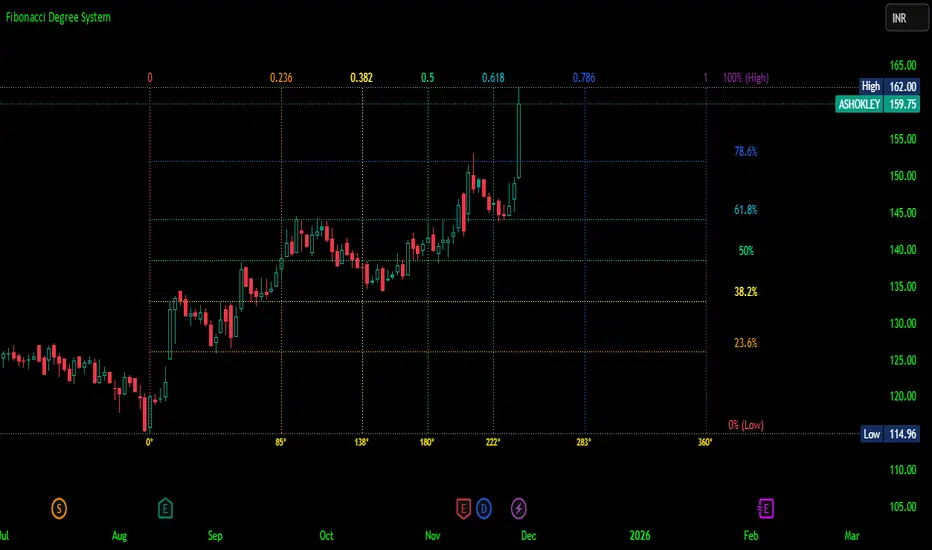
Gold Key Level LinesOverview
Gold Horizontal Lines is a visual grid tool that draws automatic horizontal levels around the current price. It’s designed for symbols like Gold (XAUUSD), but works on any market and timeframe.
What It Does
Draws main, mid, and quarter price levels based on user-defined intervals (e.g. 100 / 50 / 25).
Centers the grid around the current close, above and below by a chosen number of levels.
Adds optional price labels to each line on the right side of the chart.
Deletes and redraws lines only on the last bar to keep the chart clean and efficient.
Inputs
Main Line Interval – distance between key levels (e.g. 100).
Mid / Quarter Intervals – optional extra levels between main lines (set to 0 to disable).
Colors, Styles, Widths – separate settings for main, mid, and quarter lines.
Show Price Labels – toggle labels on/off.
Number of Lines Above/Below Price – controls how far the grid extends.

Murrey Math SMA up to 32s Murrey Math SMA up to 32s is a highly advanced Pine Script v5 indicator that combines Murrey Math Lines (MML) with a customizable moving average (MA) — including a non-repainting Rolling VWAP (RVWAP) — and dynamic color-coded support/resistance bands up to 1/32 subdivisions. It projects octave-based geometric price levels (like Gann) centered on your chosen MA, with adaptive scaling, angle-based trend coloring, and absolute/extended MML bands. Includes 1/8, 1/16, and 1/32 grid lines, shaded zones, labels, and a live increment display.Core FeaturesFeature
Description
MA Types
SMA, VWMA, VWAP, Period VWAP, RVWAP (rolling VWAP over fixed or adaptive time window)
Murrey Math Grid
Auto-scaled 0/8 to 8/8 + extensions (±3/8), with 1/16 & 1/32 subdivisions
Dynamic Coloring
Bands colored by MA slope angle (bullish/bearish) or absolute MML shift
RVWAP Engine
Non-repainting volume-weighted average over user-defined or adaptive time steps
Wick Filtering
Optional ignore wicks for cleaner MML framing
Resolution Support
Works with higher timeframe data via request.security()
Key Use Cases Use Case
How to Use
1. Precision Support & Resistance
Treat 4/8 (mid) as pivot, 0/8 & 8/8 as extremes. Price often reverses or accelerates at these levels.
2. Mean Reversion Trades
Buy near 0/8–1/8 (oversold), sell near 7/8–8/8 (overbought) when MA is flat or sloping mildly.
3. Trend Continuation
When MA angle > threshold and price breaks 5/8, expect move to 8/8. Confirm with volume.
4. Breakout Entries
Watch for close beyond 8/8 or 0/8 + MA angle steep → strong momentum breakout.
5. Scalping with 1/32 Grid
Use 1/32 lines as micro-targets in ranging markets or after news spikes.
6. Volume-Weighted Fair Value
RVWAP = true average price paid over time → anchor for institutional fair value.
Visual Layout (MA-Centered)
+3/8 ───┐
+2/8 ───┤ ← Strong resistance
+1/8 ───┤
8/8 ███┤ ← Overbought (red zone)
7/8 ───┤
6/8 ███┤
5/8 ───┤
4/8 ███┤ ← Midline (pivot)
3/8 ───┤
2/8 ███┤
1/8 ───┤
0/8 ███┤ ← Oversold (green zone)
-1/8 ───┤
-2/8 ───┤
-3/8 ───┘
Shaded: 0/8–1/8 (buy), 7/8–8/8 (sell), 3/8–5/8 (neutral/consolidation)
MA Line: Orange (RVWAP) or hidden
Labels: Bottom, 1/4, Mid, 3/4, Top (offset to the right)
Table: Shows current Increment size
Best For Swing & scalp traders on stocks, forex, crypto
Volume-based strategies (RVWAP shines in high-volume moves)
Gann/Murrey Math enthusiasts wanting automation + modern MA anchoring

EM Visible Range Volume Profile█ OVERVIEW
ᴇᴍ VRVP (Visible Range Volume Profile) indicator calculates the volume profile within the visible range of prices.
Volume Profile is an advanced technical analysis indicator that shows trading activity over a specified period of time at certain price levels.
The indicator plots a histogram on the chart that reflects dominant or significant price levels based that are based on volume.
VP concept
VP Components
Open, High, Low, Close:
There are different types of volume profile indicators but the majority of them will designate the OHLC.
Point of Control:
A price level with the most traded volume during one session, also known as POC.
High Volume Node (HVN):
Area of high volume relative to surrounding price action.
Low Volume Node (LVN):
Area of low volume relative to surrounding price action.
Analysis of price in relation to high and low volume nodes is useful when building context around your trades.
█ VOLUME PROFILE STRATEGIES
The distribution of a volume profile can help you determine the strength of a trend and spot potential reversal zones. Let’s take a look at the five different distribution types.
Neutral D
In order for price to break away from value, either the buyers or the sellers will have to become more aggressive than the other side. When this occurs, it gives us with a vital piece of information.
Now we know who were the agressors at this price level: either the buyers or the sellers. That's why this is a good level for a trading setup if the price bounces back.
Bearish P and Bullish P
Bearish P — reversal. Bullish P — confirmation.
Bearish Ь and Bullish Ь
Bearish Ь — confirmation. Bullish Ь — reversal.
Examples
█ INPUTS
Width — amplitude of the VP histogram.
Grid — the number of columns of the VP histogram.
Delta of volumes — combinatorial determination of the ratios of sellers and buyers.
In quoted units — conversion in units of quoted currency.
Logarithmic scale — recalculation the grid step to the logarithmic scale of the chart.
HTF — (Higher Timeframe) calculation of VP for the period of the selected timeframe. ISO: Isolated computation in HTF period.
Palette: Total volume, Volume of buyers, Volume of sellers, HTF bars.
Warnings: colour of the «⚠» icon, language of information in the Tooltip.
Addition: ᴇᴍ CHN-RMA — a grid of moving averages with periods of centered hexagonal numbers.
█ ОБЩИЕ СВЕДЕНИЯ
ᴇᴍ VRVP (Visible Range Volume Profile) рассчитывает профиль объёма в видимом диапазоне цен.
Профиль объёма — это продвинутый индикатор технического анализа, который показывает торговую активность за условленный период времени на определённых ценовых уровнях.
Индикатор строит на графике гистограмму, отражающую доминирующие или значимые ценовые уровни, основанные на объёме.
█ НАСТРОЙКИ
Ширина — амплитуда гистограммы VP.
Сетка — количество колонок гистограммы VP.
Дельта объёмов — комбинаторное определение соотношений продаж и покупок.
В котируемых единицах — пересчёт в единицах котируемой валюты.
Логарифмическая шкала — пересчёт шага сетки на логарифмическую шкалу графика.
HTF — (Higher Timeframe) расчёт VP за период выбранного таймфрейма. ISO: Изолированное вычисление в HTF-периоде.
Палитра: Суммарный объём, Объём покупок, Объём продаж, Бары HTF.
Предупреждения: цвет значка «⚠», язык информации в Tooltip.
Дополнение: ᴇᴍ CHN-RMA — сетка скользящих средних с периодами центрированных гексагональных чисел.