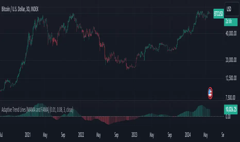
Adaptive Trend Lines [MAMA and FAMA]Updated my previous algo on the Adaptive Trend lines, however I have added new functionalities and sorted out the settings.
You can now switch between normalized and non-normalized settings, the colors have also been updated and look much better.
The MAMA and FAMA
These indicators was originally developed by John F. Ehlers (Stocks & Commodities V. 19:10: MESA Adaptive Moving Averages). Everget wrote the initial functions for these in pine script. I have simply normalized the indicators and chosen to use the Laplace transformation instead of the hilbert transformation
How the Indicator Works:
The indicator employs a series of complex calculations, but we'll break it down into key steps to understand its functionality:
LaplaceTransform: Calculates the Laplace distribution for the given src input. The Laplace distribution is a continuous probability distribution, also known as the double exponential distribution. I use this because of the assymetrical return profile
MESA Period: The indicator calculates a MESA period, which represents the dominant cycle length in the price data. This period is continuously adjusted to adapt to market changes.
InPhase and Quadrature Components: The InPhase and Quadrature components are derived from the Hilbert Transform output. These components represent different aspects of the price's cyclical behavior.
Homodyne Discriminator: The Homodyne Discriminator is a phase-sensitive technique used to determine the phase and amplitude of a signal. It helps in detecting trend changes.
Alpha Calculation: Alpha represents the adaptive factor that adjusts the sensitivity of the indicator. It is based on the MESA period and the phase of the InPhase component. Alpha helps in dynamically adjusting the indicator's responsiveness to changes in market conditions.
MAMA and FAMA Calculation: The MAMA and FAMA values are calculated using the adaptive factor (alpha) and the input price data. These values are essentially adaptive moving averages that aim to capture the current trend more effectively than traditional moving averages.
But Omar, why would anyone want to use this?
The MAMA and FAMA lines offer benefits:
The indicator offers a distinct advantage over conventional moving averages due to its adaptive nature, which allows it to adjust to changing market conditions. This adaptability ensures that investors can stay on the right side of the trend, as the indicator becomes more responsive during trending periods and less sensitive in choppy or sideways markets.
One of the key strengths of this indicator lies in its ability to identify trends effectively by combining the MESA and MAMA techniques. By doing so, it efficiently filters out market noise, making it highly valuable for trend-following strategies. Investors can rely on this feature to gain clearer insights into the prevailing trends and make well-informed trading decisions.
This indicator is primarily suppoest to be used on the big timeframes to see which trend is prevailing, however I am not against someone using it on a timeframe below the 1D, just be careful if you are using this for modern portfolio theory, this is not suppoest to be a mid-term component, but rather a long term component that works well with proper use of detrended fluctuation analysis.
Dont hesitate to ask me if you have any questions
Again, I want to give credit to Everget and ChartPrime!
Code explanation as required by House Rules:
fastLimit = input.float(title='Fast Limit', step=0.01, defval=0.01, group = "Indicator Settings")
slowLimit = input.float(title='Slow Limit', step=0.01, defval=0.08, group = "Indicator Settings")
src = input(title='Source', defval=close, group = "Indicator Settings")
input.float: Used to create input fields for the user to set the fastLimit and slowLimit values.
input: General function to get user inputs, like the data source (close price) used for calculations.
norm_period = input.int(3, 'Normalization Period', 1, group = "Normalized Settings")
norm = input.bool(defval = true, title = "Use normalization", group = "Normalized Settings")
input.int: Creates an input field for the normalization period.
input.bool: Allows the user to toggle normalization on or off.
Color settings in the code:
col_up = input.color(#22ab94, group = "Color Settings")
col_dn = input.color(#f7525f, group = "Color Settings")
Constants and functions
var float PI = math.pi
laplace(src) =>
(0.5) * math.exp(-math.abs(src))
_computeComponent(src, mesaPeriodMult) =>
out = laplace(src) * mesaPeriodMult
out
_smoothComponent(src) =>
out = 0.2 * src + 0.8 * nz(src )
out
math.pi: Represents the mathematical constant π (pi).
laplace: A function that applies the Laplace transform to the source data.
_computeComponent: Computes a component of the data using the Laplace transform.
_smoothComponent: Smooths data by averaging the current value with the previous one (nz function is used to handle null values).
Alpha function:
_computeAlpha(src, fastLimit, slowLimit) =>
mesaPeriod = 0.0
mesaPeriodMult = 0.075 * nz(mesaPeriod ) + 0.54
...
alpha = math.max(fastLimit / deltaPhase, slowLimit)
out = alpha
out
_computeAlpha: Calculates the adaptive alpha value based on the fastLimit and slowLimit. This value is crucial for determining the MAMA and FAMA lines.
Calculating MAMA and FAMA:
mama = 0.0
mama := alpha * src + (1 - alpha) * nz(mama )
fama = 0.0
fama := alpha2 * mama + (1 - alpha2) * nz(fama )
Normalization:
lowest = ta.lowest(mama_fama_diff, norm_period)
highest = ta.highest(mama_fama_diff, norm_period)
normalized = (mama_fama_diff - lowest) / (highest - lowest) - 0.5
ta.lowest and ta.highest: Find the lowest and highest values of mama_fama_diff over the normalization period.
The oscillator is normalized to a range, making it easier to compare over different periods.
And finally, the plotting:
plot(norm == true ? normalized : na, style=plot.style_columns, color=col_wn, title = "mama_fama_diff Oscillator Normalized")
plot(norm == false ? mama_fama_diff : na, style=plot.style_columns, color=col_wnS, title = "mama_fama_diff Oscillator")
Example of Normalized settings:
Example for setup:
Try to make sure the lower timeframe follows the higher timeframe if you take a trade based on this indicator!
Search in scripts for "harmonic"
Unmitigated Liquidity Imbalances [AlgoAlpha]🎉 Introducing the Unmitigated Liquidity Imbalance Indicator by AlgoAlpha! 🎉
Dive into the depths of market analytics with our "Unmitigated Liquidity Imbalance" indicator. This tool harnesses unique algorithms to detect liquidity imbalances between bulls and bears, helping traders spot trends and potential entry and exit points with greater accuracy. 📈🚀
🔍 Key Features:
🌟 Advanced Analysis : Analyses candle direction and length to forecast market peaks and valleys.
🎨 Customizable Visuals : Tailor the chart with your choice of bullish green or bearish red to reflect different market conditions.
🔄 Real-Time Updates : Continuously updates to reflect live market changes.
🔔 Configurable Alerts : Set up alerts for key trading signals such as bullish and bearish reversals, as well as trend shifts.
📐 How to Use:
🛠 Add the Indicator : Add the indicator to your favourites and customize the settings to suite your needs.
📊 Market Analysis : Monitor the oscillator threshold; readings above 0.5 suggest bullish sentiment, while below 0.5 indicate bearish conditions. And reversal signals are displayed to show potential entry points.
🔔 Set Alerts : Enable notifications for reversal conditions or trend changes to seize trading opportunities without constant chart watching.
🧠 How It Works:
The core mechanism of the indicator is based on detecting changes in candlestick size and direction to identify bullish and bearish liquidity levels from the peak & valley indicator's logic. By comparing the length of a current candle to the previous one and checking the change in direction, it pinpoints moments where market sentiment could be shifting, indicating if the liquidity at that point is bullish or bearish. The script then looks at what percentage of the past few unmitigated levels are bullish or bearish based on a customizable lookback and determines the liquidity imbalance which can then be interpreted as trend.
Empower your trading with the Unmitigated Liquidity Imbalance indicator and navigate the markets with confidence and precision. 🌟💹
Happy trading, and may your charts be ever in your favour! 🥳✨
💎 Related Indicator

Dynamic Sine Wave The Dynamic Sine Wave is designed to calculate a sine wave that reflects the oscillations between the highest high and lowest low points over a specified period, providing traders with a unique perspective on market trends.
Why a Sine Wave is Relevant:
A sine wave is relevant in this context because it is a mathematical function that represents periodic oscillations, making it suitable for capturing the cyclic nature of price movements in financial markets.
By using a sine wave, this indicator highlights the repetitive patterns of price highs and lows over a specified period, which can assist traders in identifying potential trend reversals or continuations.
The sine wave's amplitude and frequency are adjusted based on the highest high and lowest low points, ensuring that it adapts to market volatility and provides a dynamic representation of price action.
Overall, the "Dynamic Sine Wave" indicator offers a unique perspective on market dynamics, helping traders make informed decisions by visualizing the ebb and flow of prices.

ABC finderI made this script a long time again and never released it. It is a ABC Pattern finding tool. You can adjust the "Bars Back" setting to include more or less bars in the pattern. I usually have it set to 10 or 15 these settings seem to work well on most assets. The scripts allows you to set up a trade box automatically and has a call out table to make prices levels more clear and easy to read. The trade box levels can be set by fixed percentage or by pattern based fib.
Hope it helps!

BEST ABCD Pattern Screener Deribit:DVOL BTC DXY scannerModified this script by Daveatt (based on Ricardo Santos Fractals)
to scan patterns in BTCUSD, ETHUSD, DVOL, DXY, DVOL/VV


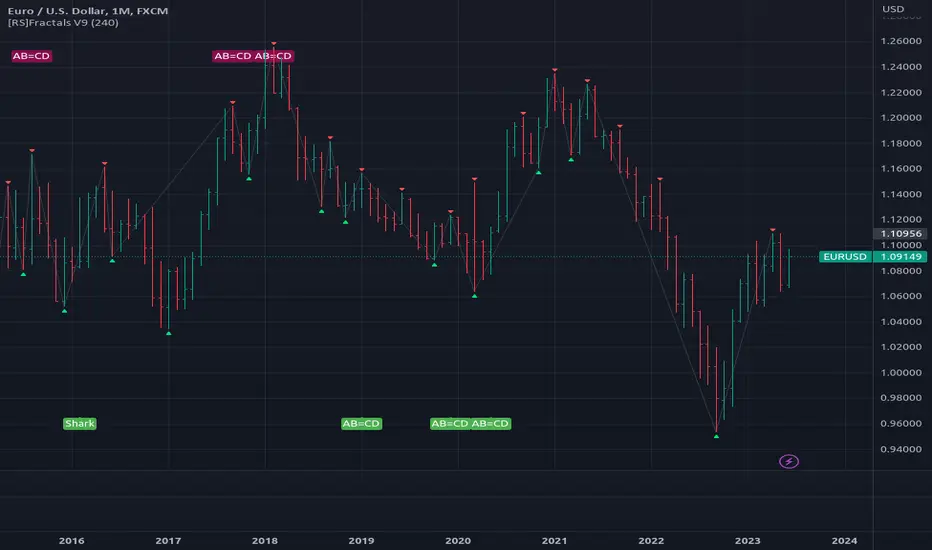
[RS]Fractals V9update: added optional option for marking the fractals with bgcolor (request for: faizal.mansor.908)

[RS]ZigZag (MA, Pattern Recognition) V2EXPERIMENTAL:
Best method so far to draw the zigzag.
Multi time frame options


Dark Cloud automatic finding scriptHi
Let me introduce my Dark Cloud automatic finding script.
This is a bearish reversal pattern formed by two candlesticks within a uptrend.
Consists of an up candlestick followed by a down candlestick which opens lower
than the prior candlestick and closes below the midrange of the prior candlestick.
It is the reverse of the Piercing Line.

Fourier series Model Of The Market█ OVERVIEW
The Fourier Series Model of the Market (FSMM) decomposes price action into harmonic components using bandpass filtering, then reconstructs a composite wave weighted by rolling energy ratios. This approach isolates cyclical market behavior at multiple frequencies, emphasizing dominant cycles for cleaner signal generation. The energy-adaptive weighting is the key differentiator from simple harmonic summation: cycles that dominate current price action contribute more to the output.
Based on Fourier analysis principles applied to financial markets, the indicator extracts harmonics (fundamental, 2nd, 3rd, etc.) using second-order IIR bandpass filters, then weights each harmonic's contribution by its relative energy compared to adjacent harmonics. This energy-adaptive weighting naturally emphasizes the cycles that are most prominent in current market conditions.
█ CONCEPTS
Fourier Decomposition
Fourier analysis represents any periodic signal as a sum of sine waves at different frequencies. In market analysis, price action can be decomposed into a fundamental cycle (the base period) plus harmonics at integer multiples of that frequency (period/2, period/3, etc.). Each harmonic captures oscillations at a specific frequency band, and their sum reconstructs the original cyclical behavior.
Bandpass Filtering
Each harmonic is extracted using a second-order IIR (Infinite Impulse Response) bandpass filter tuned to that harmonic's frequency. The filter isolates price activity within a narrow frequency range while rejecting both higher-frequency noise and lower-frequency trend drift. Before filtering, the source is debiased via 2-bar momentum to remove DC offset, ensuring each bandpass operates around true zero.
Energy-Weighted Reconstruction
Rather than simply summing all harmonics equally, FSMM weights each harmonic by its rolling energy relative to the previous harmonic. The energy score combines the current harmonic value with its rate of change, so it reflects both amplitude and momentum. Higher harmonics that hold comparatively more energy therefore contribute more to the composite wave, while weaker harmonics fade out. This adaptive weighting allows the model to respond to changing market cyclicality.
Quadrature Component (Rate of Change)
The rate of change output represents the 90°-phase-shifted (quadrature) component of the wave. When the wave is at zero and rising, the rate of change is at maximum positive. This provides complementary information about cycle phase and can be used for timing entries relative to cycle position.
█ INTERPRETATION
Wave Output
The composite wave oscillates around zero, representing the sum of all extracted harmonic components weighted by energy:
• Above zero : Net bullish cyclical momentum across harmonics
• Below zero : Net bearish cyclical momentum across harmonics
• Zero crossings : Cycle phase transitions - potential reversal points
• Wave amplitude : Strength of cyclical behavior; larger swings indicate cleaner cycles
Rate of Change
The quadrature component (90° phase-shifted) provides cycle phase information:
• Maximum rate of change : Wave is near zero and accelerating - early cycle phase
• Zero rate of change : Wave is at peak or trough - cycle extremes
• Rate/Wave divergence : When wave makes new highs/lows but rate of change does not confirm (lower momentum), suggests cycle exhaustion or impending phase shift
Combined Analysis
• Wave crossing above zero with positive rate of change: Strong bullish cycle initiation
• Wave crossing below zero with negative rate of change: Strong bearish cycle initiation
• Wave at extreme with rate of change reversing: Potential cycle peak/trough
Threshold Bands
When enabled, threshold bands define statistically significant wave deviations:
• Breach above +threshold : Unusually strong bullish cyclical behavior
• Breach below -threshold : Unusually strong bearish cyclical behavior
• Return inside thresholds : Normalizing behavior, potential mean reversion ahead
Alert Conditions
Four built-in alerts trigger on bar close (no repainting):
• Above +Threshold : Strong bullish cycle behavior
• Below -Threshold : Strong bearish cycle behavior
• Above Zero : Bullish cycle phase shift
• Below Zero : Bearish cycle phase shift
█ SETTINGS & PARAMETER TUNING
Fourier Series Model
• Source : Price series to decompose into harmonic components.
• Period (6-100): Base period for the fundamental harmonic. Higher harmonics divide this period (harmonic 2 = period/2, harmonic 3 = period/3). Match to the dominant market cycle for best results. Default 20.
• Bandwidth (0.05-0.5): Bandpass filter selectivity. Lower values create narrower passbands that isolate harmonics more precisely but may miss slightly off-frequency cycles. Higher values capture broader ranges but reduce harmonic separation. Default 0.1 balances precision and robustness.
• Harmonics (1-20): Number of harmonic components to extract. More harmonics capture finer cyclical detail but increase computation. For most applications, 3-5 harmonics suffice. The fundamental alone (1 harmonic) functions as a simple bandpass filter.
Display Settings
• Wave Outputs : Toggle visibility and color of the composite Fourier wave.
• Rate of Change : Toggle visibility and color of the quadrature component (90° phase-shifted wave).
• Zero Line : Reference line for oscillator neutrality.
Diagnostics - Dynamic Thresholds
Optional significance bands that identify when wave readings indicate strong cyclical behavior:
• Dynamic Threshold : Toggle threshold bands and set colors.
• Threshold Mode : Select calculation method:
- MAD (Median Absolute Deviation) : Robust, outlier-resistant measure using k * MAD where MAD ≈ 0.6745 * stdev.
- Standard Deviation : Volatility-sensitive, calculated as k * stdev of wave over the lookback period.
- Percentile Rank : Fixed probability bands using percentile of |wave| (90% means only 10% of values exceed threshold).
• Period (2-200): Lookback for threshold calculations. Default 50.
• Multiplier (k) : Scaling for MAD/Standard Deviation modes. Default 1.5.
• Percentile (%) (0-100): For Percentile Rank mode only. Default 90%.
Parameter Interactions
• Shorter periods respond faster to cycle changes but may capture noise.
• Lower bandwidth + more harmonics = more precise decomposition but requires accurate period setting.
• Higher bandwidth is more forgiving of period mismatches.
• For strongly trending markets, restrict harmonics to 1-2 so the model tracks the dominant cycle with fewer higher-frequency components.
• For ranging/oscillating markets, more harmonics (4-6) capture complex cycles.
█ LIMITATIONS
Inherent Characteristics
• Period dependency : Effectiveness depends on correctly matching the Period parameter to actual market cycles. Use cycle measurement tools (autocorrelation, FFT, dominant cycle indicators) to identify appropriate periods.
• Stationarity assumption : The indicator assumes cycle frequencies remain relatively stable within the lookback window. Rapidly shifting dominant cycles (regime transitions) may produce inconsistent results until the buffer adapts.
• Filter lag : Despite bandpass design, some lag remains inherent to causal filtering. Higher harmonics have less lag but more noise sensitivity.
• Energy weighting artifacts : During regime changes when harmonic energy ratios shift rapidly, weighting may produce transient anomalies.
Market Conditions to Avoid
• Strong trending markets : Pure trends with no cyclicality produce weak, meandering signals. The indicator assumes cyclical market behavior.
• News events/gaps : Large discontinuities disrupt filter continuity. Requires 1-2 full periods to stabilize.
• Period mismatch : If the Period parameter doesn't match actual market cycles, harmonic extraction produces noise rather than signal.
Parameter Selection Pitfalls
• Too many harmonics : Beyond 5-6 harmonics, additional components often capture noise rather than meaningful cycles.
• Bandwidth too narrow : Very low bandwidth (< 0.05) requires extremely precise period matching; slight mismatches cause signal loss.
• Over-optimization : Perfect historical parameter fits typically fail forward. Use robust defaults across multiple instruments.
█ NOTES
Credits
This indicator applies Fourier analysis principles to financial market data, building on the extensive work of Dr. John F. Ehlers in applying digital signal processing to trading. The bandpass filter implementation and harmonic decomposition approach draw from DSP fundamentals as presented in Ehlers' publications.
For those interested in the underlying mathematics and DSP concepts:
• Ehlers, J.F. (2001). Rocket Science for Traders: Digital Signal Processing Applications . John Wiley & Sons.
• Ehlers, J.F. (2013). Cycle Analytics for Traders . John Wiley & Sons.
• Various TASC articles by John Ehlers on bandpass filters, cycle analysis, and harmonic decomposition.
by ♚@e2e4

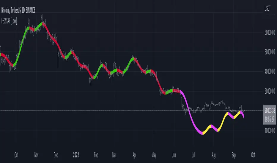
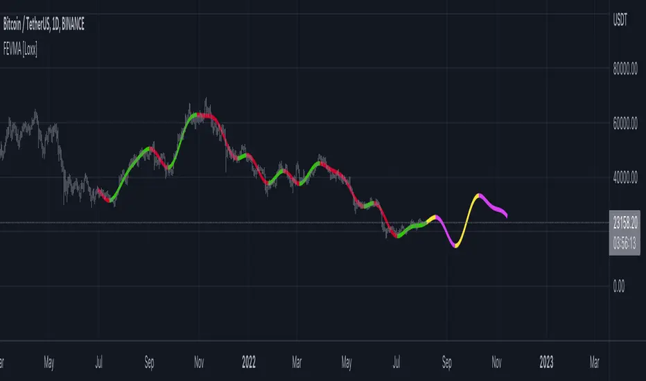
Fourier Extrapolator of 'Caterpillar' SSA of Price [Loxx]Fourier Extrapolator of 'Caterpillar' SSA of Price is a forecasting indicator that applies Singular Spectrum Analysis to input price and then injects that transformed value into the Quinn-Fernandes Fourier Transform algorithm to generate a price forecast. The indicator plots two curves: the green/red curve indicates modeled past values and the yellow/fuchsia dotted curve indicates the future extrapolated values.
What is the Fourier Transform Extrapolator of price?
Fourier Extrapolator of Price is a multi-harmonic (or multi-tone) trigonometric model of a price series xi, i=1..n, is given by:
xi = m + Sum( a*Cos(w*i) + b*Sin(w*i), h=1..H )
Where:
xi - past price at i-th bar, total n past prices;
m - bias;
a and b - scaling coefficients of harmonics;
w - frequency of a harmonic ;
h - harmonic number;
H - total number of fitted harmonics.
Fitting this model means finding m, a, b, and w that make the modeled values to be close to real values. Finding the harmonic frequencies w is the most difficult part of fitting a trigonometric model. In the case of a Fourier series, these frequencies are set at 2*pi*h/n. But, the Fourier series extrapolation means simply repeating the n past prices into the future.
Quinn-Fernandes algorithm find sthe harmonic frequencies. It fits harmonics of the trigonometric series one by one until the specified total number of harmonics H is reached. After fitting a new harmonic , the coded algorithm computes the residue between the updated model and the real values and fits a new harmonic to the residue.
see here: A Fast Efficient Technique for the Estimation of Frequency , B. G. Quinn and J. M. Fernandes, Biometrika, Vol. 78, No. 3 (Sep., 1991), pp . 489-497 (9 pages) Published By: Oxford University Press
Fourier Transform Extrapolator of Price inputs are as follows:
npast - number of past bars, to which trigonometric series is fitted;
nharm - total number of harmonics in model;
frqtol - tolerance of frequency calculations.
What is Singular Spectrum Analysis ( SSA )?
Singular spectrum analysis ( SSA ) is a technique of time series analysis and forecasting. It combines elements of classical time series analysis, multivariate statistics, multivariate geometry, dynamical systems and signal processing. SSA aims at decomposing the original series into a sum of a small number of interpretable components such as a slowly varying trend, oscillatory components and a ‘structureless’ noise. It is based on the singular value decomposition ( SVD ) of a specific matrix constructed upon the time series. Neither a parametric model nor stationarity-type conditions have to be assumed for the time series. This makes SSA a model-free method and hence enables SSA to have a very wide range of applicability.
For our purposes here, we are only concerned with the "Caterpillar" SSA . This methodology was developed in the former Soviet Union independently (the ‘iron curtain effect’) of the mainstream SSA . The main difference between the main-stream SSA and the "Caterpillar" SSA is not in the algorithmic details but rather in the assumptions and in the emphasis in the study of SSA properties. To apply the mainstream SSA , one often needs to assume some kind of stationarity of the time series and think in terms of the "signal plus noise" model (where the noise is often assumed to be ‘red’). In the "Caterpillar" SSA , the main methodological stress is on separability (of one component of the series from another one) and neither the assumption of stationarity nor the model in the form "signal plus noise" are required.
"Caterpillar" SSA
The basic "Caterpillar" SSA algorithm for analyzing one-dimensional time series consists of:
Transformation of the one-dimensional time series to the trajectory matrix by means of a delay procedure (this gives the name to the whole technique);
Singular Value Decomposition of the trajectory matrix;
Reconstruction of the original time series based on a number of selected eigenvectors.
This decomposition initializes forecasting procedures for both the original time series and its components. The method can be naturally extended to multidimensional time series and to image processing.
The method is a powerful and useful tool of time series analysis in meteorology, hydrology, geophysics, climatology and, according to our experience, in economics, biology, physics, medicine and other sciences; that is, where short and long, one-dimensional and multidimensional, stationary and non-stationary, almost deterministic and noisy time series are to be analyzed.
"Caterpillar" SSA inputs are as follows:
lag - How much lag to introduce into the SSA algorithm, the higher this number the slower the process and smoother the signal
ncomp - Number of Computations or cycles of of the SSA algorithm; the higher the slower
ssapernorm - SSA Period Normalization
numbars =- number of past bars, to which SSA is fitted
Included:
Bar coloring
Alerts
Signals
Loxx's Expanded Source Types
Related Fourier Transform Indicators
Real-Fast Fourier Transform of Price w/ Linear Regression
Fourier Extrapolator of Variety RSI w/ Bollinger Bands
Fourier Extrapolator of Price w/ Projection Forecast
Related Projection Forecast Indicators
Itakura-Saito Autoregressive Extrapolation of Price
Helme-Nikias Weighted Burg AR-SE Extra. of Price
Related SSA Indicators
End-pointed SSA of FDASMA
End-pointed SSA of Williams %R
Fourier Extrapolation of Variety Moving Averages [Loxx]Fourier Extrapolation of Variety Moving Averages is a Fourier Extrapolation (forecasting) indicator that has for inputs 38 different types of moving averages along with 33 different types of sources for those moving averages. This is a forecasting indicator of the selected moving average of the selected price of the underlying ticker. This indicator will repaint, so past signals are only as valid as the current bar. This indicator allows for up to 1500 bars between past bars and future projection bars. If the indicator won't load on your chart. check the error message for details on how to fix that, but you must ensure that past bars + futures bars is equal to or less than 1500.
Fourier Extrapolation using the Quinn-Fernandes algorithm is one of several (5-10) methods of signals forecasting that I'l be demonstrating in Pine Script.
What is Fourier Extrapolation?
This indicator uses a multi-harmonic (or multi-tone) trigonometric model of a price series xi, i=1..n, is given by:
xi = m + Sum( a*Cos(w*i) + b*Sin(w*i), h=1..H )
Where:
xi - past price at i-th bar, total n past prices;
m - bias;
a and b - scaling coefficients of harmonics;
w - frequency of a harmonic ;
h - harmonic number;
H - total number of fitted harmonics.
Fitting this model means finding m, a, b, and w that make the modeled values to be close to real values. Finding the harmonic frequencies w is the most difficult part of fitting a trigonometric model. In the case of a Fourier series, these frequencies are set at 2*pi*h/n. But, the Fourier series extrapolation means simply repeating the n past prices into the future.
This indicator uses the Quinn-Fernandes algorithm to find the harmonic frequencies. It fits harmonics of the trigonometric series one by one until the specified total number of harmonics H is reached. After fitting a new harmonic , the coded algorithm computes the residue between the updated model and the real values and fits a new harmonic to the residue.
see here: A Fast Efficient Technique for the Estimation of Frequency , B. G. Quinn and J. M. Fernandes, Biometrika, Vol. 78, No. 3 (Sep., 1991), pp . 489-497 (9 pages) Published By: Oxford University Press
The indicator has the following input parameters:
src - input source
npast - number of past bars, to which trigonometric series is fitted;
Nfut - number of predicted future bars;
nharm - total number of harmonics in model;
frqtol - tolerance of frequency calculations.
Included:
Loxx's Expanded Source Types
Loxx's Moving Averages
Other indicators using this same method
Fourier Extrapolator of Variety RSI w/ Bollinger Bands
Fourier Extrapolator of Price w/ Projection Forecast
Fourier Extrapolator of Price
Loxx's Moving Averages: Detailed explanation of moving averages inside this indicator
Loxx's Expanded Source Types: Detailed explanation of source types used in this indicator
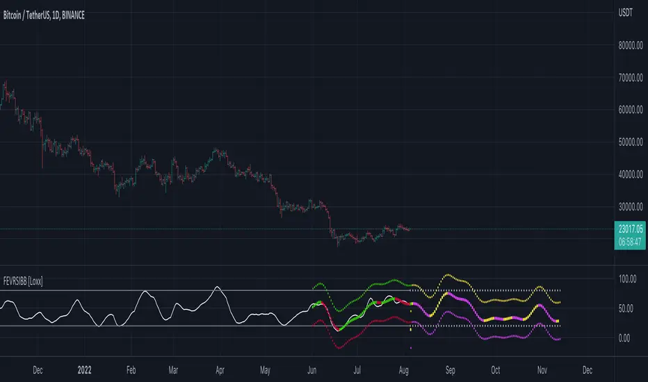
Fourier Extrapolator of Variety RSI w/ Bollinger Bands [Loxx]Fourier Extrapolator of Variety RSI w/ Bollinger Bands is an RSI indicator that shows the original RSI, the Fourier Extrapolation of RSI in the past, and then the projection of the Fourier Extrapolated RSI for the future. This indicator has 8 different types of RSI including a new type of RSI called T3 RSI. The purpose of this indicator is to demonstrate the Fourier Extrapolation method used to model past data and to predict future price movements. This indicator will repaint. If you wish to use this for trading, then make sure to take a screenshot of the indicator when you enter the trade to save your analysis. This is the first of a series of forecasting indicators that can be used in trading. Due to how this indicator draws on the screen, you must choose values of npast and nfut that are equal to or less than 200. this is due to restrictions by TradingView and Pine Script in only allowing 500 lines on the screen at a time. Enjoy!
What is Fourier Extrapolation?
This indicator uses a multi-harmonic (or multi-tone) trigonometric model of a price series xi, i=1..n, is given by:
xi = m + Sum( a*Cos(w*i) + b*Sin(w*i), h=1..H )
Where:
xi - past price at i-th bar, total n past prices;
m - bias;
a and b - scaling coefficients of harmonics;
w - frequency of a harmonic ;
h - harmonic number;
H - total number of fitted harmonics.
Fitting this model means finding m, a, b, and w that make the modeled values to be close to real values. Finding the harmonic frequencies w is the most difficult part of fitting a trigonometric model. In the case of a Fourier series, these frequencies are set at 2*pi*h/n. But, the Fourier series extrapolation means simply repeating the n past prices into the future.
This indicator uses the Quinn-Fernandes algorithm to find the harmonic frequencies. It fits harmonics of the trigonometric series one by one until the specified total number of harmonics H is reached. After fitting a new harmonic , the coded algorithm computes the residue between the updated model and the real values and fits a new harmonic to the residue.
see here: A Fast Efficient Technique for the Estimation of Frequency , B. G. Quinn and J. M. Fernandes, Biometrika, Vol. 78, No. 3 (Sep., 1991), pp . 489-497 (9 pages) Published By: Oxford University Press
The indicator has the following input parameters:
src - input source
npast - number of past bars, to which trigonometric series is fitted;
Nfut - number of predicted future bars;
nharm - total number of harmonics in model;
frqtol - tolerance of frequency calculations.
Included:
Loxx's Expanded Source Types
Loxx's Variety RSI
Other indicators using this same method
Fourier Extrapolator of Price w/ Projection Forecast
Fourier Extrapolator of Price
Frequency Momentum Oscillator [QuantAlgo]🟢 Overview
The Frequency Momentum Oscillator applies Fourier-based spectral analysis principles to price action to identify regime shifts and directional momentum. It calculates Fourier coefficients for selected harmonic frequencies on detrended price data, then measures the distribution of power across low, mid, and high frequency bands to distinguish between persistent directional trends and transient market noise. This approach provides traders with a quantitative framework for assessing whether current price action represents meaningful momentum or merely random fluctuations, enabling more informed entry and exit decisions across various asset classes and timeframes.
🟢 How It Works
The calculation process removes the dominant trend from price data by subtracting a simple moving average, isolating cyclical components for frequency analysis:
detrendedPrice = close - ta.sma(close , frequencyPeriod)
The detrended price series undergoes frequency decomposition through Fourier coefficient calculation across the first 8 harmonics. For each harmonic frequency, the algorithm computes sine and cosine components across the lookback window, then derives power as the sum of squared coefficients:
for k = 1 to 8
cosSum = 0.0
sinSum = 0.0
for n = 0 to frequencyPeriod - 1
angle = 2 * math.pi * k * n / frequencyPeriod
cosSum := cosSum + detrendedPrice * math.cos(angle)
sinSum := sinSum + detrendedPrice * math.sin(angle)
power = (cosSum * cosSum + sinSum * sinSum) / frequencyPeriod
Power measurements are aggregated into three frequency bands: low frequencies (harmonics 1-2) capturing persistent cycles, mid frequencies (harmonics 3-4), and high frequencies (harmonics 5-8) representing noise. Each band's power normalizes against total spectral power to create percentage distributions:
lowFreqNorm = totalPower > 0 ? (lowFreqPower / totalPower) * 100 : 33.33
highFreqNorm = totalPower > 0 ? (highFreqPower / totalPower) * 100 : 33.33
The normalized frequency components undergo exponential smoothing before calculating spectral balance as the difference between low and high frequency power:
smoothLow = ta.ema(lowFreqNorm, smoothingPeriod)
smoothHigh = ta.ema(highFreqNorm, smoothingPeriod)
spectralBalance = smoothLow - smoothHigh
Spectral balance combines with price momentum through directional multiplication, producing a composite signal that integrates frequency characteristics with price direction:
momentum = ta.change(close , frequencyPeriod/2)
compositeSignal = spectralBalance * math.sign(momentum)
finalSignal = ta.ema(compositeSignal, smoothingPeriod)
The final signal oscillates around zero, with positive values indicating low-frequency dominance coupled with upward momentum (trending up), and negative values indicating either high-frequency dominance (choppy market) or downward momentum (trending down).
🟢 How to Use This Indicator
→ Long/Short Signals: the indicator generates long signals when the smoothed composite signal crosses above zero (indicating low-frequency directional strength dominates) and short signals when it crosses below zero (indicating bearish momentum persistence).
→ Upper and Lower Reference Lines: the +25 and -25 reference lines serve as threshold markers for momentum strength. Readings beyond these levels indicate strong directional conviction, while oscillations between them suggest consolidation or weakening momentum. These references help traders distinguish between strong trending regimes and choppy transitional periods.
→ Preconfigured Presets: three optimized configurations are available with Default (32, 3) offering balanced responsiveness, Fast Response (24, 2) designed for scalping and intraday trading, and Smooth Trend (40, 5) calibrated for swing trading and position trading with enhanced noise filtration.
→ Built-in Alerts: the indicator includes three alert conditions for automated monitoring - Long Signal (momentum shifts bullish), Short Signal (momentum shifts bearish), and Signal Change (any directional transition). These alerts enable traders to receive real-time notifications without continuous chart monitoring.
→ Color Customization: four visual themes (Classic green/red, Aqua blue/orange, Cosmic aqua/purple, Custom) allow chart customization for different display environments and personal preferences.

The Abramelin Protocol [MPL]"Any sufficiently advanced technology is indistinguishable from magic." — Arthur C. Clarke
🌑 SYSTEM OVERVIEW
The Abramelin Protocol is not a standard technical indicator; it is a "Technomantic" trading algorithm engineered to bridge the gap between 15th-century esoteric mathematics and modern high-frequency markets.
This script is the flagship implementation of the MPL (Magic Programming Language) project—an open-source experimental framework designed to compile metaphysical intent into executable Python and Pine Script algorithms.
Unlike traditional indicators that rely on arbitrary constants (like the 14-period RSI or 200 SMA), this protocol calculates its parameters using "Dynamic Entity Gematria." We utilize a custom Python backend to analyze the ASCII vibrational frequencies of specific metaphysical archetypes, reducing them via Tesla's 3-6-9 harmonic principles to derive market-responsive periods.
🧬 WHAT IS ?
MPL (Magic Programming Language) is a domain-specific language and research initiative created to explore Technomancy—the art of treating code as a spellbook and the market as a chaotic entity to be tamed.
By integrating the logic of ancient Grimoires (such as The Book of Abramelin) with modern Data Science, MPL aims to discover hidden correlations in price action that standard tools overlook.
🔗 CONNECT WITH THE PROJECT:
If you are a developer, a trader, or a seeker of hidden knowledge, examine the source code and join the order:
• 📂 Official Project Site: hakanovski.github.io
• 🐍 MPL Source Code (GitHub): github.com
• 👨💻 Developer Profile (LinkedIn): www.linkedin.com
🔢 THE ALGORITHM: 452 - 204 - 50
The inputs for this script are mathematically derived signatures of the intelligence governing the system:
1. THE PAIMON TREND (Gravity)
• Origin: Derived from the ASCII summation of the archetype PAIMON (King of Secret Knowledge).
• Function: This 452-period Baseline acts as the market's "Event Horizon." It represents the deep, structural direction of the asset.
• Price > Line: Bullish Domain.
• Price < Line: Bearish Void.
2. THE ASTAROTH SIGNAL (Trigger)
• Origin: Derived from the ASCII summation of ASTAROTH (Knower of Past & Future), reduced by Tesla’s 3rd Harmonic.
• Function: This is the active trigger line. It replaces standard moving averages with a precise, gematria-aligned trajectory.
3. THE VOLATILITY MATRIX (Scalp)
• Origin: Based on the 9th Harmonic reduction.
• Function: Creates a "Cloud" around the signal line to visualize market noise.
🛡️ THE MILON GATE (Matrix Filter)
Unique to this script is the "MILON Gate" toggle found in the settings.
• ☑️ Active (Default): The algorithm applies the logic of the MILON Magic Square. Signals are ONLY generated if Volume and Volatility align with the geometric structure of the move. This filters out ~80% of false signals (noise).
• ⬜ Inactive: The algorithm operates in "Raw Mode," showing every mathematical crossover without the volume filter.
⚠️ OPERATIONAL USAGE
• Timeframe: Optimized for 4H (The Builder) and Daily (The Architect) charts.
• Strategy: Use the Black/Grey Line (452) as your directional bias. Take entries only when the "EXECUTE" (Long) or "PURGE" (Short) sigils appear.
Use this tool wisely. Risk responsibly. Let the harmonics guide your entries.
— Hakan Yorganci
Technomancer & Full Stack Developer

Quinn-Fernandes Fourier Transform of Filtered Price [Loxx]Down the Rabbit Hole We Go: A Deep Dive into the Mysteries of Quinn-Fernandes Fast Fourier Transform and Hodrick-Prescott Filtering
In the ever-evolving landscape of financial markets, the ability to accurately identify and exploit underlying market patterns is of paramount importance. As market participants continuously search for innovative tools to gain an edge in their trading and investment strategies, advanced mathematical techniques, such as the Quinn-Fernandes Fourier Transform and the Hodrick-Prescott Filter, have emerged as powerful analytical tools. This comprehensive analysis aims to delve into the rich history and theoretical foundations of these techniques, exploring their applications in financial time series analysis, particularly in the context of a sophisticated trading indicator. Furthermore, we will critically assess the limitations and challenges associated with these transformative tools, while offering practical insights and recommendations for overcoming these hurdles to maximize their potential in the financial domain.
Our investigation will begin with a comprehensive examination of the origins and development of both the Quinn-Fernandes Fourier Transform and the Hodrick-Prescott Filter. We will trace their roots from classical Fourier analysis and time series smoothing to their modern-day adaptive iterations. We will elucidate the key concepts and mathematical underpinnings of these techniques and demonstrate how they are synergistically used in the context of the trading indicator under study.
As we progress, we will carefully consider the potential drawbacks and challenges associated with using the Quinn-Fernandes Fourier Transform and the Hodrick-Prescott Filter as integral components of a trading indicator. By providing a critical evaluation of their computational complexity, sensitivity to input parameters, assumptions about data stationarity, performance in noisy environments, and their nature as lagging indicators, we aim to offer a balanced and comprehensive understanding of these powerful analytical tools.
In conclusion, this in-depth analysis of the Quinn-Fernandes Fourier Transform and the Hodrick-Prescott Filter aims to provide a solid foundation for financial market participants seeking to harness the potential of these advanced techniques in their trading and investment strategies. By shedding light on their history, applications, and limitations, we hope to equip traders and investors with the knowledge and insights necessary to make informed decisions and, ultimately, achieve greater success in the highly competitive world of finance.
█ Fourier Transform and Hodrick-Prescott Filter in Financial Time Series Analysis
Financial time series analysis plays a crucial role in making informed decisions about investments and trading strategies. Among the various methods used in this domain, the Fourier Transform and the Hodrick-Prescott (HP) Filter have emerged as powerful techniques for processing and analyzing financial data. This section aims to provide a comprehensive understanding of these two methodologies, their significance in financial time series analysis, and their combined application to enhance trading strategies.
█ The Quinn-Fernandes Fourier Transform: History, Applications, and Use in Financial Time Series Analysis
The Quinn-Fernandes Fourier Transform is an advanced spectral estimation technique developed by John J. Quinn and Mauricio A. Fernandes in the early 1990s. It builds upon the classical Fourier Transform by introducing an adaptive approach that improves the identification of dominant frequencies in noisy signals. This section will explore the history of the Quinn-Fernandes Fourier Transform, its applications in various domains, and its specific use in financial time series analysis.
History of the Quinn-Fernandes Fourier Transform
The Quinn-Fernandes Fourier Transform was introduced in a 1993 paper titled "The Application of Adaptive Estimation to the Interpolation of Missing Values in Noisy Signals." In this paper, Quinn and Fernandes developed an adaptive spectral estimation algorithm to address the limitations of the classical Fourier Transform when analyzing noisy signals.
The classical Fourier Transform is a powerful mathematical tool that decomposes a function or a time series into a sum of sinusoids, making it easier to identify underlying patterns and trends. However, its performance can be negatively impacted by noise and missing data points, leading to inaccurate frequency identification.
Quinn and Fernandes sought to address these issues by developing an adaptive algorithm that could more accurately identify the dominant frequencies in a noisy signal, even when data points were missing. This adaptive algorithm, now known as the Quinn-Fernandes Fourier Transform, employs an iterative approach to refine the frequency estimates, ultimately resulting in improved spectral estimation.
Applications of the Quinn-Fernandes Fourier Transform
The Quinn-Fernandes Fourier Transform has found applications in various fields, including signal processing, telecommunications, geophysics, and biomedical engineering. Its ability to accurately identify dominant frequencies in noisy signals makes it a valuable tool for analyzing and interpreting data in these domains.
For example, in telecommunications, the Quinn-Fernandes Fourier Transform can be used to analyze the performance of communication systems and identify interference patterns. In geophysics, it can help detect and analyze seismic signals and vibrations, leading to improved understanding of geological processes. In biomedical engineering, the technique can be employed to analyze physiological signals, such as electrocardiograms, leading to more accurate diagnoses and better patient care.
Use of the Quinn-Fernandes Fourier Transform in Financial Time Series Analysis
In financial time series analysis, the Quinn-Fernandes Fourier Transform can be a powerful tool for isolating the dominant cycles and frequencies in asset price data. By more accurately identifying these critical cycles, traders can better understand the underlying dynamics of financial markets and develop more effective trading strategies.
The Quinn-Fernandes Fourier Transform is used in conjunction with the Hodrick-Prescott Filter, a technique that separates the underlying trend from the cyclical component in a time series. By first applying the Hodrick-Prescott Filter to the financial data, short-term fluctuations and noise are removed, resulting in a smoothed representation of the underlying trend. This smoothed data is then subjected to the Quinn-Fernandes Fourier Transform, allowing for more accurate identification of the dominant cycles and frequencies in the asset price data.
By employing the Quinn-Fernandes Fourier Transform in this manner, traders can gain a deeper understanding of the underlying dynamics of financial time series and develop more effective trading strategies. The enhanced knowledge of market cycles and frequencies can lead to improved risk management and ultimately, better investment performance.
The Quinn-Fernandes Fourier Transform is an advanced spectral estimation technique that has proven valuable in various domains, including financial time series analysis. Its adaptive approach to frequency identification addresses the limitations of the classical Fourier Transform when analyzing noisy signals, leading to more accurate and reliable analysis. By employing the Quinn-Fernandes Fourier Transform in financial time series analysis, traders can gain a deeper understanding of the underlying financial instrument.
Drawbacks to the Quinn-Fernandes algorithm
While the Quinn-Fernandes Fourier Transform is an effective tool for identifying dominant cycles and frequencies in financial time series, it is not without its drawbacks. Some of the limitations and challenges associated with this indicator include:
1. Computational complexity: The adaptive nature of the Quinn-Fernandes Fourier Transform requires iterative calculations, which can lead to increased computational complexity. This can be particularly challenging when analyzing large datasets or when the indicator is used in real-time trading environments.
2. Sensitivity to input parameters: The performance of the Quinn-Fernandes Fourier Transform is dependent on the choice of input parameters, such as the number of harmonic periods, frequency tolerance, and Hodrick-Prescott filter settings. Choosing inappropriate parameter values can lead to inaccurate frequency identification or reduced performance. Finding the optimal parameter settings can be challenging, and may require trial and error or a more sophisticated optimization process.
3. Assumption of stationary data: The Quinn-Fernandes Fourier Transform assumes that the underlying data is stationary, meaning that its statistical properties do not change over time. However, financial time series data is often non-stationary, with changing trends and volatility. This can limit the effectiveness of the indicator and may require additional preprocessing steps, such as detrending or differencing, to ensure the data meets the assumptions of the algorithm.
4. Limitations in noisy environments: Although the Quinn-Fernandes Fourier Transform is designed to handle noisy signals, its performance may still be negatively impacted by significant noise levels. In such cases, the identification of dominant frequencies may become less reliable, leading to suboptimal trading signals or strategies.
5. Lagging indicator: As with many technical analysis tools, the Quinn-Fernandes Fourier Transform is a lagging indicator, meaning that it is based on past data. While it can provide valuable insights into historical market dynamics, its ability to predict future price movements may be limited. This can result in false signals or late entries and exits, potentially reducing the effectiveness of trading strategies based on this indicator.
Despite these drawbacks, the Quinn-Fernandes Fourier Transform remains a valuable tool for financial time series analysis when used appropriately. By being aware of its limitations and adjusting input parameters or preprocessing steps as needed, traders can still benefit from its ability to identify dominant cycles and frequencies in financial data, and use this information to inform their trading strategies.
█ Deep-dive into the Hodrick-Prescott Fitler
The Hodrick-Prescott (HP) filter is a statistical tool used in economics and finance to separate a time series into two components: a trend component and a cyclical component. It is a powerful tool for identifying long-term trends in economic and financial data and is widely used by economists, central banks, and financial institutions around the world.
The HP filter was first introduced in the 1990s by economists Robert Hodrick and Edward Prescott. It is a simple, two-parameter filter that separates a time series into a trend component and a cyclical component. The trend component represents the long-term behavior of the data, while the cyclical component captures the shorter-term fluctuations around the trend.
The HP filter works by minimizing the following objective function:
Minimize: (Sum of Squared Deviations) + λ (Sum of Squared Second Differences)
Where:
1. The first term represents the deviation of the data from the trend.
2. The second term represents the smoothness of the trend.
3. λ is a smoothing parameter that determines the degree of smoothness of the trend.
The smoothing parameter λ is typically set to a value between 100 and 1600, depending on the frequency of the data. Higher values of λ lead to a smoother trend, while lower values lead to a more volatile trend.
The HP filter has several advantages over other smoothing techniques. It is a non-parametric method, meaning that it does not make any assumptions about the underlying distribution of the data. It also allows for easy comparison of trends across different time series and can be used with data of any frequency.
Another significant advantage of the HP Filter is its ability to adapt to changes in the underlying trend. This feature makes it particularly well-suited for analyzing financial time series, which often exhibit non-stationary behavior. By employing the HP Filter to smooth financial data, traders can more accurately identify and analyze the long-term trends that drive asset prices, ultimately leading to better-informed investment decisions.
However, the HP filter also has some limitations. It assumes that the trend is a smooth function, which may not be the case in some situations. It can also be sensitive to changes in the smoothing parameter λ, which may result in different trends for the same data. Additionally, the filter may produce unrealistic trends for very short time series.
Despite these limitations, the HP filter remains a valuable tool for analyzing economic and financial data. It is widely used by central banks and financial institutions to monitor long-term trends in the economy, and it can be used to identify turning points in the business cycle. The filter can also be used to analyze asset prices, exchange rates, and other financial variables.
The Hodrick-Prescott filter is a powerful tool for analyzing economic and financial data. It separates a time series into a trend component and a cyclical component, allowing for easy identification of long-term trends and turning points in the business cycle. While it has some limitations, it remains a valuable tool for economists, central banks, and financial institutions around the world.
█ Combined Application of Fourier Transform and Hodrick-Prescott Filter
The integration of the Fourier Transform and the Hodrick-Prescott Filter in financial time series analysis can offer several benefits. By first applying the HP Filter to the financial data, traders can remove short-term fluctuations and noise, effectively isolating the underlying trend. This smoothed data can then be subjected to the Fourier Transform, allowing for the identification of dominant cycles and frequencies with greater precision.
By combining these two powerful techniques, traders can gain a more comprehensive understanding of the underlying dynamics of financial time series. This enhanced knowledge can lead to the development of more effective trading strategies, better risk management, and ultimately, improved investment performance.
The Fourier Transform and the Hodrick-Prescott Filter are powerful tools for financial time series analysis. Each technique offers unique benefits, with the Fourier Transform being adept at identifying dominant cycles and frequencies, and the HP Filter excelling at isolating long-term trends from short-term noise. By combining these methodologies, traders can develop a deeper understanding of the underlying dynamics of financial time series, leading to more informed investment decisions and improved trading strategies. As the financial markets continue to evolve, the combined application of these techniques will undoubtedly remain an essential aspect of modern financial analysis.
█ Features
Endpointed and Non-repainting
This is an endpointed and non-repainting indicator. These are crucial factors that contribute to its usefulness and reliability in trading and investment strategies. Let us break down these concepts and discuss why they matter in the context of a financial indicator.
1. Endpoint nature: An endpoint indicator uses the most recent data points to calculate its values, ensuring that the output is timely and reflective of the current market conditions. This is in contrast to non-endpoint indicators, which may use earlier data points in their calculations, potentially leading to less timely or less relevant results. By utilizing the most recent data available, the endpoint nature of this indicator ensures that it remains up-to-date and relevant, providing traders and investors with valuable and actionable insights into the market dynamics.
2. Non-repainting characteristic: A non-repainting indicator is one that does not change its values or signals after they have been generated. This means that once a signal or a value has been plotted on the chart, it will remain there, and future data will not affect it. This is crucial for traders and investors, as it offers a sense of consistency and certainty when making decisions based on the indicator's output.
Repainting indicators, on the other hand, can change their values or signals as new data comes in, effectively "repainting" the past. This can be problematic for several reasons:
a. Misleading results: Repainting indicators can create the illusion of a highly accurate or successful trading system when backtesting, as the indicator may adapt its past signals to fit the historical price data. This can lead to overly optimistic performance results that may not hold up in real-time trading.
b. Decision-making uncertainty: When an indicator repaints, it becomes challenging for traders and investors to trust its signals, as the signal that prompted a trade may change or disappear after the fact. This can create confusion and indecision, making it difficult to execute a consistent trading strategy.
The endpoint and non-repainting characteristics of this indicator contribute to its overall reliability and effectiveness as a tool for trading and investment decision-making. By providing timely and consistent information, this indicator helps traders and investors make well-informed decisions that are less likely to be influenced by misleading or shifting data.
Inputs
Source: This input determines the source of the price data to be used for the calculations. Users can select from options like closing price, opening price, high, low, etc., based on their preferences. Changing the source of the price data (e.g., from closing price to opening price) will alter the base data used for calculations, which may lead to different patterns and cycles being identified.
Calculation Bars: This input represents the number of past bars used for the calculation. A higher value will use more historical data for the analysis, while a lower value will focus on more recent price data. Increasing the number of past bars used for calculation will incorporate more historical data into the analysis. This may lead to a more comprehensive understanding of long-term trends but could also result in a slower response to recent price changes. Decreasing this value will focus more on recent data, potentially making the indicator more responsive to short-term fluctuations.
Harmonic Period: This input represents the harmonic period, which is the number of harmonics used in the Fourier Transform. A higher value will result in more harmonics being used, potentially capturing more complex cycles in the price data. Increasing the harmonic period will include more harmonics in the Fourier Transform, potentially capturing more complex cycles in the price data. However, this may also introduce more noise and make it harder to identify clear patterns. Decreasing this value will focus on simpler cycles and may make the analysis clearer, but it might miss out on more complex patterns.
Frequency Tolerance: This input represents the frequency tolerance, which determines how close the frequencies of the harmonics must be to be considered part of the same cycle. A higher value will allow for more variation between harmonics, while a lower value will require the frequencies to be more similar. Increasing the frequency tolerance will allow for more variation between harmonics, potentially capturing a broader range of cycles. However, this may also introduce noise and make it more difficult to identify clear patterns. Decreasing this value will require the frequencies to be more similar, potentially making the analysis clearer, but it might miss out on some cycles.
Number of Bars to Render: This input determines the number of bars to render on the chart. A higher value will result in more historical data being displayed, but it may also slow down the computation due to the increased amount of data being processed. Increasing the number of bars to render on the chart will display more historical data, providing a broader context for the analysis. However, this may also slow down the computation due to the increased amount of data being processed. Decreasing this value will speed up the computation, but it will provide less historical context for the analysis.
Smoothing Mode: This input allows the user to choose between two smoothing modes for the source price data: no smoothing or Hodrick-Prescott (HP) smoothing. The choice depends on the user's preference for how the price data should be processed before the Fourier Transform is applied. Choosing between no smoothing and Hodrick-Prescott (HP) smoothing will affect the preprocessing of the price data. Using HP smoothing will remove some of the short-term fluctuations from the data, potentially making the analysis clearer and more focused on longer-term trends. Not using smoothing will retain the original price fluctuations, which may provide more detail but also introduce noise into the analysis.
Hodrick-Prescott Filter Period: This input represents the Hodrick-Prescott filter period, which is used if the user chooses to apply HP smoothing to the price data. A higher value will result in a smoother curve, while a lower value will retain more of the original price fluctuations. Increasing the Hodrick-Prescott filter period will result in a smoother curve for the price data, emphasizing longer-term trends and minimizing short-term fluctuations. Decreasing this value will retain more of the original price fluctuations, potentially providing more detail but also introducing noise into the analysis.
Alets and signals
This indicator featues alerts, signals and bar coloring. You have to option to turn these on/off in the settings menu.
Maximum Bars Restriction
This indicator requires a large amount of processing power to render on the chart. To reduce overhead, the setting "Number of Bars to Render" is set to 500 bars. You can adjust this to you liking.
█ Related Indicators and Libraries
Goertzel Cycle Composite Wave
Goertzel Browser
Fourier Spectrometer of Price w/ Extrapolation Forecast
Fourier Extrapolator of 'Caterpillar' SSA of Price
Normalized, Variety, Fast Fourier Transform Explorer
Real-Fast Fourier Transform of Price Oscillator
Real-Fast Fourier Transform of Price w/ Linear Regression
Fourier Extrapolation of Variety Moving Averages
Fourier Extrapolator of Variety RSI w/ Bollinger Bands
Fourier Extrapolator of Price w/ Projection Forecast
Fourier Extrapolator of Price
STD-Stepped Fast Cosine Transform Moving Average
Variety RSI of Fast Discrete Cosine Transform
loxfft

ahpuhelperLibrary "ahpuhelper"
Helper Library for Auto Harmonic Patterns UltimateX. It is not meaningful for others. This is supposed to be private library. But, publishing it to make sure that I don't delete accidentally. Some functions may be useful for coders.
insert_open_trades_table_column(showOpenTrades, table_id, column, colors, values, intStatus, harmonicTrailingStartState, lblSizeOpenTrades)
add data to open trades table column
Parameters:
showOpenTrades : flag to show open trades table
table_id : Table Id
column : refers to pattern data
colors : backgroud and text color array
values : cell values
intStatus : status as integer
harmonicTrailingStartState : trailing Start state as per configs
lblSizeOpenTrades : text size
Returns: nextColumn
populate_closed_stats(ClosedStatsPosition, bullishCounts, bearishCounts, bullishRetouchCounts, bearishRetouchCounts, bullishSizeMatrix, bearishSizeMatrix, bullishRR, bearishRR, allPatternLabels, flags, rowMain, rowHeaders)
populate closed stats for harmonic patterns
Parameters:
ClosedStatsPosition : Table position for closed stats
bullishCounts : Matrix containing bullish trade stats
bearishCounts : Matrix containing bearish trade stats
bullishRetouchCounts : Matrix containing bullish trade stats for those which retouched entry
bearishRetouchCounts : Matrix containing bearish trade stats for those which retouched entry
bullishSizeMatrix : Matrix containing data about size of bullish patterns
bearishSizeMatrix : Matrix containing data about size of bearish patterns
bullishRR : Matrix containing Risk Reward data of bullish patterns
bearishRR : Matrix containing Risk Reward data of bearish patterns
allPatternLabels : array containing pattern labels
flags : display flags
rowMain : Pattern header data
rowHeaders : header grouping data
Returns: void
get_rr_details(patternTradeDetails, harmonicTrailingStartState, disableTrail, breakEvenTrail)
calculate and return risk reward based on targets and stops
Parameters:
patternTradeDetails : array containing stop, entry and targets
harmonicTrailingStartState : trailing point
disableTrail : If set, ignores trailing point
breakEvenTrail : If set, trailing does not go beyond breakeven.
Returns: nextColumn

Momentum Echo Oscillator [Community Edition]Concept: The Momentum Echo Oscillator (MEO) is a modern take on classical momentum oscillators. Most indicators only look at the "now". MEO introduces the concept of Momentum Echoes—historical momentum harmonics that are weighted and blended back into the current price velocity.
Why use MEO? Standard momentum tools (like ROC or RSI) can be very "jittery" or noisy. By integrating historical echoes, MEO provides a smoother, more rhythmic representation of price flow, making it easier to spot genuine trend reversals.
Key Elements:
Primary Momentum: The immediate speed of price.
Echo Harmonics: Two adjustable lookback points that act as a "memory" for the indicator, filtering out false breakouts.
Dynamic Histogram: Visualizes the gap between the Echo Engine and the Trigger Line, highlighting acceleration and deceleration.
Settings:
Echo Weight: Adjust how much "memory" you want the indicator to have.
Smoothing: Clean up the signals for higher timeframes.
This is an open-source tool for the TradingView community. Enjoy!

Vassago & Tesla Ex-Machina 197 45 21 [Hakan Yorganci]Vassago & Tesla Ex-Machina 197 45 21
"Any sufficiently advanced technology is indistinguishable from magic." — Arthur C. Clarke
🌑 The Genesis: Algorithmic Esotericism
This script is not merely a technical indicator; it is a digital artifact born from the convergence of Software Engineering and Hermetic Tradition.
As a developer and researcher dedicated to "Technomancy"—the study of applying esoteric logic to computational systems—I designed this algorithm using a custom, experimental programming environment I am currently developing. My goal was to move beyond standard, arbitrary financial inputs (like the default 200 SMA or 14 RSI) and instead derive parameters based on Universal Harmonics and Historical Archetypes.
This indicator, Ex-Machina, is the result of that transmutation. It applies ancient numeric precision to modern market chaos.
🔢 Decoding the Protocol: 197 - 45 - 21
Why these specific numbers? They were not chosen randomly; they were calculated through specific harmonic reductions to filter out market noise.
1. The Harmonic Trend (Tesla Protocol)
* The Logic: Standard analysis uses the 200-period Moving Average simply out of habit. However, applying Nikola Tesla’s 3-6-9 vibrational principles, the engine reduced the period to 197.
* The Numerology: 1+9+7 = 17 \rightarrow 1+7 = \mathbf{8}. In esoteric numerology, 8 represents infinite power, authority, and financial flow. This creates a baseline that aligns more organically with market accumulation than the static 200.
2. The Hidden Dip (Solomonic Sight)
* The Archetype: Based on the attributes of Vassago, the archetype of discovering "hidden things," the algorithm identified 45 as the precise threshold for a "Sniper Entry."
* The Function: Unlike the standard 30 RSI, this level identifies the exact moment a correction matures within a bullish trend—catching the dip before the crowd returns.
3. The Prophetic Vision
* The Logic: Using the Fibonacci Sequence, the indicator projects the support line 21 bars into the future.
* The Utility: This allows you to visualize where the support will be, granting you foresight before price action arrives.
⚖️ The Dual Mode Engine: Sealed vs. Living
Respecting the user's will, I have engineered this script as a Hybrid System. You can choose how the "spirit" of the code interacts with the market via the settings menu.
1. The Sealed Ritual (Default - Unchecked)
* Philosophy: "Trust in the Constants."
* Behavior: Strictly adheres to the 197 SMA and 45 RSI.
* Visual: Displays a Blue Trend Line.
* Best For: Traders who value stability, long-term trends, and the unyielding nature of harmonic mathematics.
2. The Living Spirit (Adaptive Mode - Checked)
* Philosophy: "As the market breathes, so does the code."
* Behavior:
* Transmutation: The trend line shifts from a Simple Moving Average (SMA) to an Exponential Moving Average (EMA 197) for faster reaction.
* Adaptive Volatility: The RSI entry level (45) becomes dynamic. It expands and contracts based on ATR (Average True Range). In high volatility, it demands a deeper dip to trigger a signal, protecting you from fake-outs.
* Visual: Displays a Fuchsia (Pink) Trend Line.
* Best For: Volatile markets (Crypto/Forex) and traders who want the algorithm to "sense" the fear and greed in the air.
⚙️ How to Trade
* Timeframe: Optimized for 4H (The Builder) and 1D (The Architect).
* The Signal: Wait for the "EX-MACHINA ENTRY" label. This signal manifests ONLY when:
* Price is holding above the 197 Harmonic Trend.
* Momentum crosses the Optimized Threshold (45 or Adaptive).
* Trend Strength is confirmed via ADX.
Author's Note:
I built this tool for those who understand that code is the modern spellbook. Use it wisely, risk responsibly, and let the harmonics guide your entries.
— Hakan Yorganci
Technomancer & Full Stack Developer

Jenkins Square Root Levels Square Root Levels with Fixed Spacing (Extended Lines)
This script calculates and displays horizontal levels based on the square root of a price point. It offers two calculation modes, Octave System and Square Root Multiples, allowing traders to identify key support and resistance levels derived from price harmonics.
The methodology is inspired by the teachings of Michael Jenkins, to whom I owe much gratitude for sharing his profound insights into the geometric principles of trading.
Features and Functions
1. Calculation Modes
Octave System:
Divides the square root range into specified steps, called "octave divisions."
Each division calculates levels proportionally or evenly spaced, depending on the selected spacing mode.
Multiple repetitions (or multiples) extend these levels upward, downward, or both.
Square Root Multiples:
Adds or subtracts multiples of the square root of the price point to create levels.
These multiples act as harmonics of the original square root, providing meaningful levels for price action.
2. Spacing Modes
Proportional: Levels are scaled proportionally with each multiple, resulting in increasing spacing as multiples grow.
Even: Levels are spaced equally, maintaining a consistent distance regardless of the multiple.
3. Direction
Up: Calculates levels above the price point only.
Down: Calculates levels below the price point only.
Both: Displays levels on both sides of the price point.
4. Customization Options
Price Point: Enter any key high, low, or other significant price point to anchor the calculations.
Octave Division: Adjust the number of divisions within the octave (e.g., 4 for quarter-steps, 8 for eighth-steps).
Number of Multiples: Set how far the levels should extend (e.g., 3 for 3 repetitions of the octave or square root multiples).
5. Visualization
The calculated levels are plotted as horizontal lines that extend across the chart.
Lines are sorted and plotted dynamically for clarity, with spacing adjusted according to the chosen parameters.
Acknowledgments
This script is based on the trading methodologies and geometric insights shared by Michael S. Jenkins. His work has profoundly influenced my understanding of price action and the role of harmonics in trading. Thank you, Michael Jenkins, for your invaluable teachings.