WLSMA: fast approximation🙏🏻 Sup TV & @alexgrover
O(N) algocomplexity, just one loop inside. No, you can't do O(1) @ updates in moving window mode, only expanding window will allow that.
Now I have time series & stats models of my own creation, nowhere else available, just TV and my github for now, ain’t no legacy academic industry I always have fun about, but back in 2k20 when I consciously ain’t known much about quant, I remember seeing post by @alexgrover recreating Moving Regression Endpoint dropped on price chart (called LSMA here) as a linear filter combination of filters (yea yeah DSP terms) as 3WMA - 2SMA. Now it’s my time to do smth alike aye?
...
This script is remake of my 1st degree WLSMA via linear filter combo. It’s much faster, we aint calculate moving regression per se, we just match its freq response. You can see it on the screen (WLSMAfa) almost perfectly matching the original one (WLSMA).
...
While humans like to overfit, I fw generalizations. So your lovely WMA is actually just one case of a more general weight pattern: pow(len - i, e), where pow is the power function and e is the exponent itself. So:
- If e = 0, then we have SMA (every number in 0th power is one)
- If e = 1, we get WMA
- If e = 2, we get quadratic weights.
We can recreate WLSMA freq response then by combining 2 filters with e = 1 and e = 2.
This is still an approximation, even tho enormously precise for the tasks you’ve shared with me. Due to the non-linear nature of the thing it’s all we can do, and as window size grows, even this small discrepancy converges with true WLSMA value, so we’re all good. Pls don’t try to model this 0.00xxxx discrepancy, it’s not natural.
...
DSP approach is unnatural for prices, but you can put this thing on volume delta and be happy, or on other metrics of yours, if for some reason u dont wanna estimate thresholds by fitting a distro.
All good TV
∞
P.S.: strangely, the first script made & dropped in the location in Saint P where my actual quant way has started ~5 years ago xD, very thankful
Search in scripts for "one一季度财报"

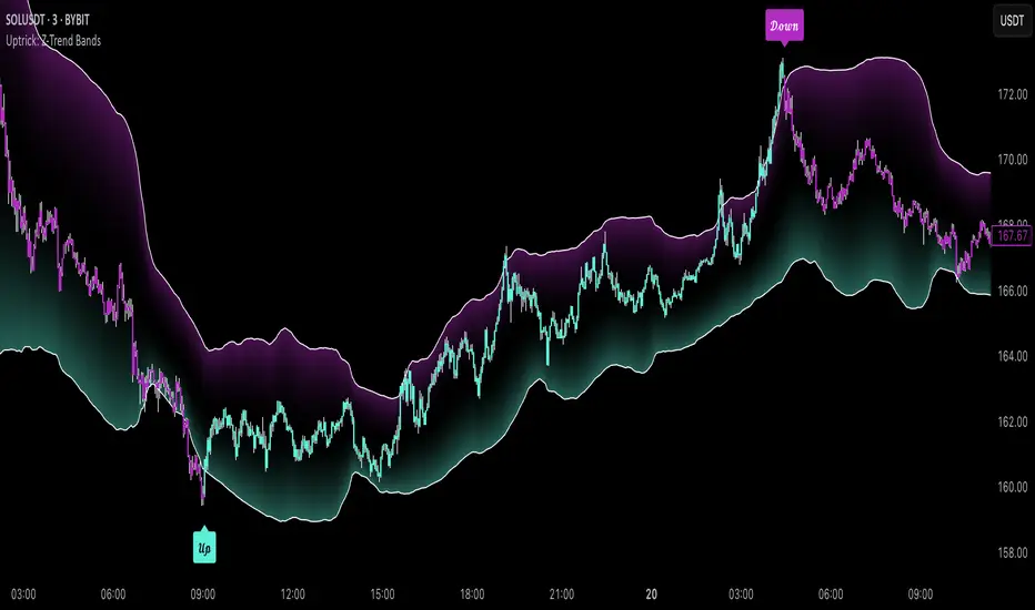
Uptrick: Z-Trend BandsOverview
Uptrick: Z-Trend Bands is a Pine Script overlay crafted to capture high-probability mean-reversion opportunities. It dynamically plots upper and lower statistical bands around an EMA baseline by converting price deviations into z-scores. Once price moves outside these bands and then reenters, the indicator verifies that momentum is genuinely reversing via an EMA-smoothed RSI slope. Signal memory ensures only one entry per momentum swing, and traders receive clear, real-time feedback through customizable bar-coloring modes, a semi-transparent fill highlighting the statistical zone, concise “Up”/“Down” labels, and a live five-metric scoring table.
Introduction
Markets often oscillate between trending and reverting, and simple thresholds or static envelopes frequently misfire when volatility shifts. Standard deviation quantifies how “wide” recent price moves have been, and a z-score transforms each deviation into a measure of how rare it is relative to its own history. By anchoring these bands to an exponential moving average, the script maintains a fluid statistical envelope that adapts instantly to both calm and turbulent regimes. Meanwhile, the Relative Strength Index (RSI) tracks momentum; smoothing RSI with an EMA and observing its slope filters out erratic spikes, ensuring that only genuine momentum flips—upward for longs and downward for shorts—qualify.
Purpose
This indicator is purpose-built for short-term mean-reversion traders operating on lower–timeframe charts. It reveals when price has strayed into the outer 5 percent of its recent range, signaling an increased likelihood of a bounce back toward fair value. Rather than firing on price alone, it demands that momentum follow suit: the smoothed RSI slope must flip in the opposite direction before any trade marker appears. This dual-filter approach dramatically reduces noise-driven, false setups. Traders then see immediate visual confirmation—bar colors that reflect the latest signal and age over time, clear entry labels, and an always-visible table of metric scores—so they can gauge both the validity and freshness of each signal at a glance.
Originality and Uniqueness
Uptrick: Z-Trend Bands stands apart from typical envelope or oscillator tools in four key ways. First, it employs fully normalized z-score bands, meaning ±2 always captures roughly the top and bottom 5 percent of moves, regardless of volatility regime. Second, it insists on two simultaneous conditions—price reentry into the bands and a confirming RSI slope flip—dramatically reducing whipsaw signals. Third, it uses slope-phase memory to lock out duplicate signals until momentum truly reverses again, enforcing disciplined entries. Finally, it offers four distinct bar-coloring schemes (solid reversal, fading reversal, exceeding bands, and classic heatmap) plus a dynamic scoring table, rather than a single, opaque alert, giving traders deep insight into every layer of analysis.
Why Each Component Was Picked
The EMA baseline was chosen for its blend of responsiveness—weighting recent price heavily—and smoothness, which filters market noise. Z-score deviation bands standardize price extremes relative to their own history, adapting automatically to shifting volatility so that “extreme” always means statistically rare. The RSI, smoothed with an EMA before slope calculation, captures true momentum shifts without the false spikes that raw RSI often produces. Slope-phase memory flags prevent repeated alerts within a single swing, curbing over-trading in choppy conditions. Bar-coloring modes provide flexible visual contexts—whether you prefer to track the latest reversal, see signal age, highlight every breakout, or view a continuous gradient—and the scoring table breaks down all five core checks for complete transparency.
Features
This indicator offers a suite of configurable visual and logical tools designed to make reversal signals both robust and transparent:
Dynamic z-score bands that expand or contract in real time to reflect current volatility regimes, ensuring the outer ±zThreshold levels always represent statistically rare extremes.
A smooth EMA baseline that weights recent price more heavily, serving as a fair-value anchor around which deviations are measured.
EMA-smoothed RSI slope confirmation, which filters out erratic momentum spikes by first smoothing raw RSI and then requiring its bar-to-bar slope to flip before any signal is allowed.
Slope-phase memory logic that locks out duplicate buy or sell markers until the RSI slope crosses back through zero, preventing over-trading during choppy swings.
Four distinct bar-coloring modes—Reversal Solid, Reversal Fade, Exceeding Bands, Classic Heat—plus a “None” option, so traders can choose whether to highlight the latest signal, show signal age, emphasize breakout bars, or view a continuous heat gradient within the bands.
A semi-transparent fill between the EMA and the upper/lower bands that visually frames the statistical zone and makes extremes immediately obvious.
Concise “Up” and “Down” labels that plot exactly when price re-enters a band with confirming momentum, keeping chart clutter to a minimum.
A real-time, five-metric scoring table (z-score, RSI slope, price vs. EMA, trend state, re-entry) that updates every two bars, displaying individual +1/–1/0 scores and an averaged Buy/Sell/Neutral verdict for complete transparency.
Calculations
Compute the fair-value EMA over fairLen bars.
Subtract that EMA from current price each bar to derive the raw deviation.
Over zLen bars, calculate the rolling mean and standard deviation of those deviations.
Convert each deviation into a z-score by subtracting the mean and dividing by the standard deviation.
Plot the upper and lower bands at ±zThreshold × standard deviation around the EMA.
Calculate raw RSI over rsiLen bars, then smooth it with an EMA of length rsiEmaLen.
Derive the RSI slope by taking the difference between the current and previous smoothed RSI.
Detect a potential reentry when price exits one of the bands on the prior bar and re-enters on the current bar.
Require that reentry coincide with an RSI slope flip (positive for a lower-band reentry, negative for an upper-band reentry).
On first valid reentry per momentum swing, fire a buy or sell signal and set a memory flag; reset that flag only when the RSI slope crosses back through zero.
For each bar, assign scores of +1, –1, or 0 for the z-score direction, RSI slope, price vs. EMA, trend-state, and reentry status.
Average those five scores; if the result exceeds +0.1, label “Buy,” if below –0.1, label “Sell,” otherwise “Neutral.”
Update bar colors, the semi-transparent fill, reversal labels, and the scoring table every two bars to reflect the latest calculations.
How It Actually Works
On each new candle, the EMA baseline and band widths update to reflect current volatility. The RSI is smoothed and its slope recalculated. The script then looks back one bar to see if price exited either band and forward to see if it reentered. If that reentry coincides with an appropriate RSI slope flip—and no signal has yet been generated in that swing—a concise label appears. Bar colors refresh according to your selected mode, and the scoring table updates to show which of the five conditions passed or failed, along with the overall verdict. This process repeats seamlessly at each bar, giving traders a continuous feed of disciplined, statistically filtered reversal cues.
Inputs
All parameters are fully user-configurable, allowing you to tailor sensitivity, lookbacks, and visuals to your trading style:
EMA length (fairLen): number of bars for the fair-value EMA; higher values smooth more but lag further behind price.
Z-Score lookback (zLen): window for calculating the mean and standard deviation of price deviations; longer lookbacks reduce noise but respond more slowly to new volatility.
Z-Score threshold (zThreshold): number of standard deviations defining the upper and lower bands; common default is 2.0 for roughly the outer 5 percent of moves.
Source (src): choice of price series (close, hl2, etc.) used for EMA, deviation, and RSI calculations.
RSI length (rsiLen): period for raw RSI calculation; shorter values react faster to momentum changes but can be choppier.
RSI EMA length (rsiEmaLen): period for smoothing raw RSI before taking its slope; higher values filter more noise.
Bar coloring mode (colorMode): select from None, Reversal Solid, Reversal Fade, Exceeding Bands, or Classic Heat to control how bars are shaded in relation to signals and band positions.
Show signals (showSignals): toggle on-chart “Up” and “Down” labels for reversal entries.
Show scoring table (enableTable): toggle the display of the five-metric breakdown table.
Table position (tablePos): choose which corner (Top Left, Top Right, Bottom Left, Bottom Right) hosts the scoring table.
Conclusion
By merging a normalized z-score framework, momentum slope confirmation, disciplined signal memory, flexible visuals, and transparent scoring into one Pine Script overlay, Uptrick: Z-Trend Bands offers a powerful yet intuitive tool for intraday mean-reversion trading. Its adaptability to real-time volatility and multi-layered filter logic deliver clear, high-confidence reversal cues without the clutter or confusion of simpler indicators.
Disclaimer
This indicator is provided solely for educational and informational purposes. It does not constitute financial advice. Trading involves substantial risk and may not be suitable for all investors. Past performance is not indicative of future results. Always conduct your own testing and apply careful risk management before trading live.
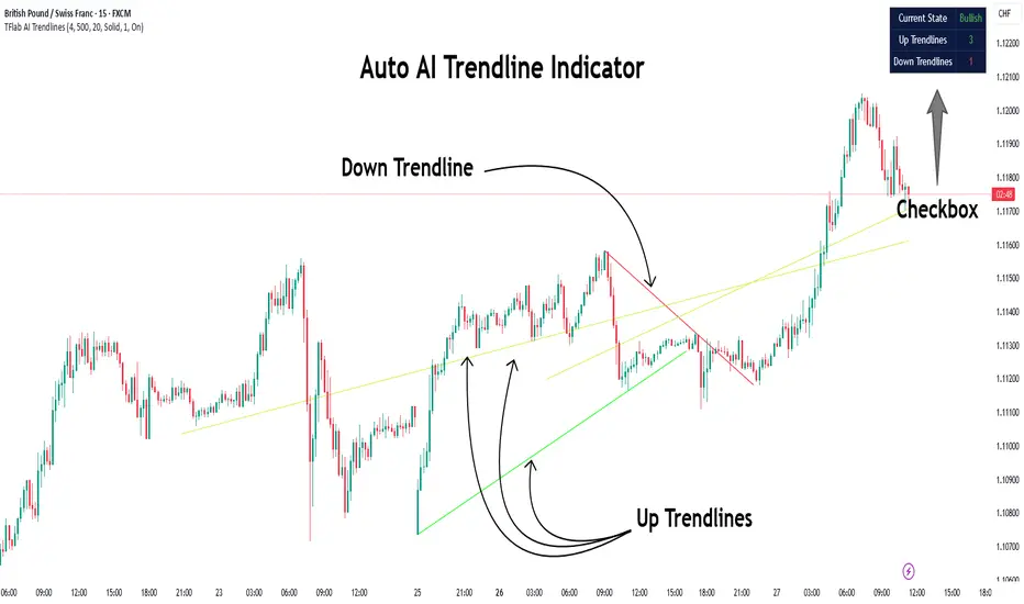
Auto AI Trendlines [TradingFinder] Clustering & Filtering Trends🔵 Introduction
Auto AI trendlines Clustering & Filtering Trends Indicator, draws a variety of trendlines. This auto plotting trendline indicator plots precise trendlines and regression lines, capturing trend dynamics.
Trendline trading is the strongest strategy in the financial market.
Regression lines, unlike trendlines, use statistical fitting to smooth price data, revealing trend slopes. Trendlines connect confirmed pivots, ensuring structural accuracy. Regression lines adapt dynamically.
The indicator’s ascending trendlines mark bullish pivots, while descending ones signal bearish trends. Regression lines extend in steps, reflecting momentum shifts. As the trend is your friend, this tool aligns traders with market flow.
Pivot-based trendlines remain fixed once confirmed, offering reliable support and resistance zones. Regression lines, adjusting to price changes, highlight short-term trend paths. Both are vital for traders across asset classes.
🔵 How to Use
There are four line types that are seen in the image below; Precise uptrend (green) and downtrend (red) lines connect exact price extremes, while Pivot-based uptrend and downtrend lines use significant swing points, both remaining static once formed.
🟣 Precise Trendlines
Trendlines only form after pivot points are confirmed, ensuring reliability. This reduces false signals in choppy markets. Regression lines complement with real-time updates.
The indicator always draws two precise trendlines on confirmed pivot points, one ascending and one descending. These are colored distinctly to mark bullish and bearish trends. They remain fixed, serving as structural anchors.
🟣 Dynamic Regression Lines
Regression lines, adjusting dynamically with price, reflect the latest trend slope for real-time analysis. Use these to identify trend direction and potential reversals.
Regression lines, updated dynamically, reflect real-time price trends and extend in steps. Ascending lines are green, descending ones orange, with shades differing from trendlines. This aids visual distinction.
🟣 Bearish Chart
A Bullish State emerges when uptrend lines outweigh or match downtrend lines, with recent upward momentum signaling a potential rise. Check the trend count in the state table to confirm, using it to plan long positions.
🟣 Bullish Chart
A Bearish State is indicated when downtrend lines dominate or equal uptrend lines, with recent downward moves suggesting a potential drop. Review the state table’s trend count to verify, guiding short position entries. The indicator reflects this shift for strategic planning.
🟣 Alarm
Set alerts for state changes to stay informed of Bullish or Bearish shifts without constant monitoring. For example, a transition to Bullish State may signal a buying opportunity. Toggle alerts On or Off in the settings.
🟣 Market Status
A table summarizes the chart’s status, showing counts of ascending and descending lines. This real-time overview simplifies trend monitoring. Check it to assess market bias instantly.
Monitor the table to track line counts and trend dominance.
A higher count of ascending lines suggests bullish bias. This helps traders align with the prevailing trend.
🔵 Settings
Number of Trendlines : Sets total lines (max 10, min 3), balancing chart clarity and trend coverage.
Max Look Back : Defines historical bars (min 50) for pivot detection, ensuring robust trendlines.
Pivot Range : Sets pivot sensitivity (min 2), adjusting trendline precision to market volatility.
Show Table Checkbox : Toggles display of a table showing ascending/descending line counts.
Alarm : Enable or Disable the alert.
🔵 Conclusion
The multi slopes indicator, blending pivot-based trendlines and dynamic regression lines, maps market trends with precision. Its dual approach captures both structural and short-term momentum.
Customizable settings, like trendline count and pivot range, adapt to diverse trading styles. The real-time table simplifies trend monitoring, enhancing efficiency. It suits forex, stocks, and crypto markets.
While trendlines anchor long-term trends, regression lines track intraday shifts, offering versatility. Contextual analysis, like price action, boosts signal reliability. This indicator empowers data-driven trading decisions.
Delta Volume Profile [BigBeluga]🔵Delta Volume Profile
A dynamic volume analysis tool that builds two separate horizontal profiles: one for bullish candles and one for bearish candles. This indicator helps traders identify the true balance of buying vs. selling volume across price levels, highlighting points of control (POCs), delta dominance, and hidden volume clusters with remarkable precision.
🔵 KEY FEATURES
Split Volume Profiles (Bull vs. Bear):
The indicator separates volume based on candle direction:
If close > open , the candle’s volume is added to the bullish profile (positive volume).
If close < open , it contributes to the bearish profile (negative volume).
ATR-Based Binning:
The price range over the selected lookback is split into bins using ATR(200) as the bin height.
Each bin accumulates both bull and bear volumes to form the dual-sided profile.
Bull and Bear Volume Bars:
Bullish volumes are shown as right-facing bars on the right side, colored with a bullish gradient.
Bearish volumes appear as left-facing bars on the left side, shaded with a bearish gradient.
Each bar includes a volume label (e.g., +12.45K or -9.33K) to show exact volume at that price level.
Points of Control (POC) Highlighting:
The bin with the highest bullish volume is marked with a border in POC+ color (default: blue).
The bin with the highest bearish volume is marked with a POC− color (default: orange).
Total Volume Density Map:
A neutral gray background box is plotted behind candles showing the total volume (bull + bear) per bin.
This reveals high-interest price zones regardless of direction.
Delta and Total Volume Summary:
A Delta label appears at the top, showing net % difference between bull and bear volume.
A Total label at the bottom shows total accumulated volume across all bins.
🔵 HOW IT WORKS
The indicator captures all candles within the lookback period .
It calculates the price range and splits it into bins using ATR for adaptive resolution.
For each candle:
If price intersects a bin and close > open , volume is added to the positive profile .
If close < open , volume is added to the negative profile .
The result is two side-by-side histograms at each price level—one for buyers, one for sellers.
The bin with the highest value on each side is visually emphasized using POC highlight colors.
At the end, the script calculates:
Delta: Total % difference between bull and bear volumes.
Total: Sum of all volumes in the lookback window.
🔵 USAGE
Volume Imbalance Zones: Identify price levels where buyers or sellers were clearly dominant.
Fade or Follow Volume Clusters: Use POC+ or POC− levels for reaction trades or breakouts.
Delta Strength Filtering: Strong delta values (> ±20%) suggest momentum or exhaustion setups.
Volume-Based Anchoring: Use profile levels to mark hidden support/resistance and execution zones.
🔵 CONCLUSION
Delta Volume Profile offers a unique advantage in market reading by separating buyer and seller activity into two visual layers. This allows traders to not only spot where volume was high, but also who was more aggressive. Whether you’re analyzing trend continuations, reversals, or absorption levels, this indicator gives you the transparency needed to trade with confidence.

UM Dual MA with Price Bar Color change & Fill
Description
This is a dual moving average indicator with colored bars and moving averages. I wrote this indicator to keep myself on the right side of the market and trends. It plots two moving averages, (length and type of MA are user-defined) and colors the MAs green when trending higher or red when trending lower. The price bars are green when both MAs are green, red when both MAs are red, and orange when one MA is green and the other is red. The idea behind the indicator is to be extremely visual. If I am buying a red bar, I ask myself "why?" If I am selling a green bar, again, "why?"
Recommended Usage
Configure your tow favorite Moving averages. Consider long positions when one or both turn green. Scale into a position with a portion upon the first MA turning green, and then more when the second turns green. Consider scaling out when the bars are orange after an up move.
Orange bars are either areas of consolidation or prior to major turns.
You can also look for MA crossovers.
The indicator works on any timeframe and any security. I use it on daily, hourly, 2 day charts.
Default settings
The defaults are the author's preferred settings:
- 8 period WMA and 16 period WMA.
- Bars are green when both MAs are trending higher, red when both MAs are trending lower, and orange when one MA is trending higher and the other is trending lower.
Moving average types, lengths, and colors are user-configurable. Bar colors are also user-configurable.
Alerts
Alerts can be set by right-clicking the indicator and selecting the dropdown:
- Bullish Trend Both MAs turning green
- Bearish Trend Both MAs turning red
- Mixed Trend, 1 green 1 red MA
Helpful Hints:
Look for bullish areas when both MAs turn green after a sustained downtrend
Look for bearish areas when both MAs turn red
Careful in areas of orange bars, this could be a consolidation or a warning to a potential trend direction change.
Switch up your timeframes, I toggle back and forth between 1 and 2 days.
Stretch your timeframe over a lower time frame; for example, I like the 8 and 16 daily WMA. With most securities I get 16 bars with pre and post market. This translates into 128 and 256 MAs on the hourly chart. This slows down moves and color transitions for better manageability.
Author's Subjective Observations
I like the 128/256 WMA on the hourly charts for leveraged and inverse ETFs such as SPXL/SPXS, TQQQ/SQQQ, TNA/TZA. Or even the volatility ETFs/ETNS: UVXY, VXX.
Here is a one-hour chart example:
I have noticed that as volatility increases, I should begin looking at higher timeframes. This seems counterintuitive, but higher volatility increases the level of noise or swings.
I question myself when I short a green bar or buy a red bar; "Why am I doing this?" The colors help me visually stay on the right side of trend. If I am going to speculate on a market turn, at least do it when the bars are orange (MA trends differ)
My last observation is a 2-day chart of leveraged ETFs with the 8 and 16 WMAs. I frequently trade SPXL, FNGA, and TNA. If you are really dissecting this indicator,
look at a few 2-day charts. 2-day charts seem to catch the major swings nicely up and down. They also weed out the daily sudden big swings such as a panic move from economic data
or tweets. When both the MAs turn red on a 2-day chart the same day or same bar, beware; this could be a rough ride or short opportunity. I found weekly charts too long for my style but good
to review for direction. Less decisions on longer charts equate to less brain damage for myself.
These are just my thoughts, of course you do you and what suits your style best! Happy Trading.

Cointegration Buy and Sell Signals [EdgeTerminal]The Cointegration Buy And Sell Signals is a sophisticated technical analysis tool to spot high-probability market turning points — before they fully develop on price charts.
Most reversal indicators rely on raw price action, visual patterns, or basic and common indicator logic — which often suffer in noisy or trending markets. In most cases, they lag behind the actual change in trend and provide useless and late signals.
This indicator is rooted in advanced concepts from statistical arbitrage, mean reversion theory, and quantitative finance, and it packages these ideas in a user-friendly visual format that works on any timeframe and asset class.
It does this by analyzing how the short-term and long-term EMAs behave relative to each other — and uses statistical filters like Z-score, correlation, volatility normalization, and stationarity tests to issue highly selective Buy and Sell signals.
This tool provides statistical confirmation of trend exhaustion, allowing you to trade mean-reverting setups. It fades overextended moves and uses signal stacking to reduce false entries. The entire indicator is based on a very interesting mathematically grounded model which I will get into down below.
Here’s how the indicator works at a high level:
EMAs as Anchors: It starts with two Exponential Moving Averages (EMAs) — one short-term and one long-term — to track market direction.
Statistical Spread (Regression Residuals): It performs a rolling linear regression between the short and long EMA. Instead of using the raw difference (short - long), it calculates the regression residual, which better models their natural relationship.
Normalize the Spread: The spread is divided by historical price volatility (ATR) to make it scale-invariant. This ensures the indicator works on low-priced stocks, high-priced indices, and crypto alike.
Z-Score: It computes a Z-score of the normalized spread to measure how “extreme” the current deviation is from its historical average.
Dynamic Thresholds: Unlike most tools that use fixed thresholds (like Z = ±2), this one calculates dynamic thresholds using historical percentiles (e.g., top 10% and bottom 10%) so that it adapts to the asset's current behavior to reduce false signals based on market’s extreme volatility at a certain time.
Z-Score Momentum: It tracks the direction of the Z-score — if Z is extreme but still moving away from zero, it's too early. It waits for reversion to start (Z momentum flips).
Correlation Check: Uses a rolling Pearson correlation to confirm the two EMAs are still statistically related. If they diverge (low correlation), no signal is shown.
Stationarity Filter (ADF-like): Uses the volatility of the regression residual to determine if the spread is stationary (mean-reverting) — a key concept in cointegration and statistical arbitrage. It’s not possible to build an exact ADF filter in Pine Script so we used the next best thing.
Signal Control: Prevents noisy charts and overtrading by ensuring no back-to-back buy or sell signals. Each signal must alternate and respect a cooldown period so you won’t be overwhelmed and won’t get a messy chart.
Important Notes to Remember:
The whole idea behind this indicator is to try to use some stat arb models to detect shifting patterns faster than they appear on common indicators, so in some cases, some assumptions are made based on historic values.
This means that in some cases, the indicator can “jump” into the conclusion too quickly. Although we try to eliminate this by using stationary filters, correlation checks, and Z-score momentum detection, there is still a chance some signals that are generated can be too early, in the stock market, that's the same as being incorrect. So make sure to use this with other indicators to confirm the movement.
How To Use The Indicator:
You can use the indicator as a standalone reversal system, as a filter for overbought and oversold setups, in combination with other trend indicators and as a part of a signal stack with other common indicators for divergence spotting and fade trades.
The indicator produces simple buy and sell signals when all criteria is met. Based on our own testing, we recommend treating these signals as standalone and independent from each other . Meaning that if you take position after a buy signal, don’t wait for a sell signal to appear to exit the trade and vice versa.
This is why we recommend using this indicator with other advanced or even simple indicators as an early confirmation tool.
The Display Table:
The floating diagnostic table in the top-right corner of the chart is a key part of this indicator. It's a live statistical dashboard that helps you understand why a signal is (or isn’t) being triggered, and whether the market conditions are lining up for a potential reversal.
1. Z-Score
What it shows: The current Z-score value of the volatility-normalized spread between the short EMA and the regression line of the long EMA.
Why it matters: Z-score tells you how statistically extreme the current relationship is. A Z-score of:
0 = perfectly average
> +2 = very overbought
< -2 = very oversold
How to use it: Look for Z-score reaching extreme highs or lows (beyond dynamic thresholds). Watch for it to start reversing direction, especially when paired with green table rows (see below)
2. Z-Score Momentum
What it shows: The rate of change (ROC) of the Z-score:
Zmomentum=Zt − Zt − 1
Why it matters: This tells you if the Z-score is still stretching out (e.g., getting more overbought/oversold), or reverting back toward the mean.
How to use it: A positive Z-momentum after a very low Z-score = potential bullish reversal A negative Z-momentum after a very high Z-score = potential bearish reversal. Avoid signals when momentum is still pushing deeper into extremes
3. Correlation
What it shows: The rolling Pearson correlation coefficient between the short EMA and long EMA.
Why it matters: High correlation (closer to +1) means the EMAs are still statistically connected — a key requirement for cointegration or mean reversion to be valid.
How to use it: Look for correlation > 0.7 for reliable signals. If correlation drops below 0.5, ignore the Z-score — the EMAs aren’t moving together anymore
4. Stationary
What it shows: A simplified "Yes" or "No" answer to the question:
“Is the spread statistically stable (stationary) and mean-reverting right now?”
Why it matters: Mean reversion strategies only work when the spread is stationary — that is, when the distance between EMAs behaves like a rubber band, not a drifting cloud.
How to use it: A "Yes" means the indicator sees a consistent, stable spread — good for trading. "No" means the market is too volatile, disjointed, or chaotic for reliable mean reversion. Wait for this to flip to "Yes" before trusting signals
5. Last Signal
What it shows: The last signal issued by the system — either "Buy", "Sell", or "None"
Why it matters: Helps avoid confusion and repeated entries. Signals only alternate — you won’t get another Buy until a Sell happens, and vice versa.
How to use it: If the last signal was a "Buy", and you’re watching for a Sell, don’t act on more bullish signals. Great for systems where you only want one position open at a time
6. Bars Since Signal
What it shows: How many bars (candles) have passed since the last Buy or Sell signal.
Why it matters: Gives you context for how long the current condition has persisted
How to use it: If it says 1 or 2, a signal just happened — avoid jumping in late. If it’s been 10+ bars, a new opportunity might be brewing soon. You can use this to time exits if you want to fade a recent signal manually
Indicator Settings:
Short EMA: Sets the short-term EMA period. The smaller the number, the more reactive and more signals you get.
Long EMA: Sets the slow EMA period. The larger this number is, the smoother baseline, and more reliable trend bases are generated.
Z-Score Lookback: The period or bars used for mean & std deviation of spread between short and long EMAs. Larger values result in smoother signals with fewer false positives.
Volatility Window: This value normalizes the spread by historical volatility. This allows you to prevent scale distortion, showing you a cleaner and better chart.
Correlation Lookback: How many periods or how far back to test correlation between slow and long EMAs. This filters out false positives when EMAs lose alignment.
Hurst Lookback: The multiplier to approximate stationarity. Lower leads to more sensitivity to regime change, higher produces a more stricter filtering.
Z Threshold Percentile: This value sets how extreme Z-score must be to trigger a signal. For example, 90 equals only top/bottom 10% of extremes, 80 = more frequent.
Min Bars Between Signals: This hard stop prevents back-to-back signals. The idea is to avoid over-trading or whipsaws in volatile markets even when Hurst lookback and volatility window values are not enough to filter signals.
Some More Recommendations:
We recommend trying different EMA pairs (10/50, 21/100, 5/20) for different asset behaviors. You can set percentile to 85 or 80 if you want more frequent but looser signals. You can also use the Z-score reversion monitor for powerful confirmation.

ADR% Extension Levels from SMA 50I created this indicator inspired by RealSimpleAriel (a swing trader I recommend following on X) who does not buy stocks extended beyond 4 ADR% from the 50 SMA and uses extensions from the 50 SMA at 7-8-9-10-11-12-13 ADR% to take profits with a 20% position trimming.
RealSimpleAriel's strategy (as I understood it):
-> Focuses on leading stocks from leading groups and industries, i.e., those that have grown the most in the last 1-3-6 months (see on Finviz groups and then select sector-industry).
-> Targets stocks with the best technical setup for a breakout, above the 200 SMA in a bear market and above both the 50 SMA and 200 SMA in a bull market, selecting those with growing Earnings and Sales.
-> Buys stocks on breakout with a stop loss set at the day's low of the breakout and ensures they are not extended beyond 4 ADR% from the 50 SMA.
-> 3-5 day momentum burst: After a breakout, takes profits by selling 1/2 or 1/3 of the position after a 3-5 day upward move.
-> 20% trimming on extension from the 50 SMA: At 7 ADR% (ADR% calculated over 20 days) extension from the 50 SMA, takes profits by selling 20% of the remaining position. Continues to trim 20% of the remaining position based on the stock price extension from the 50 SMA, calculated using the 20-period ADR%, thus trimming 20% at 8-9-10-11 ADR% extension from the 50 SMA. Upon reaching 12-13 ADR% extension from the 50 SMA, considers the stock overextended, closes the remaining position, and evaluates a short.
-> Trailing stop with ascending SMA: Uses a chosen SMA (10, 20, or 50) as the definitive stop loss for the position, depending on the stock's movement speed (preferring larger SMAs for slower-moving stocks or for long-term theses). If the stock's closing price falls below the chosen SMA, the entire position is closed.
In summary:
-->Buy a breakout using the day's low of the breakout as the stop loss (this stop loss is the most critical).
--> Do not buy stocks extended beyond 4 ADR% from the 50 SMA.
--> Sell 1/2 or 1/3 of the position after 3-5 days of upward movement.
--> Trim 20% of the position at each 7-8-9-10-11-12-13 ADR% extension from the 50 SMA.
--> Close the entire position if the breakout fails and the day's low of the breakout is reached.
--> Close the entire position if the price, during the rise, falls below a chosen SMA (10, 20, or 50, depending on your preference).
--> Definitively close the position if it reaches 12-13 ADR% extension from the 50 SMA.
I used Grok from X to create this indicator. I am not a programmer, but based on the ADR% I use, it works.
Below is Grok from X's description of the indicator:
Script Description
The script is a custom indicator for TradingView that displays extension levels based on ADR% relative to the 50-period Simple Moving Average (SMA). Below is a detailed description of its features, structure, and behavior:
1. Purpose of the Indicator
Name: "ADR% Extension Levels from SMA 50".
Objective: Draw horizontal blue lines above and below the 50-period SMA, corresponding to specific ADR% multiples (4, 7, 8, 9, 10, 11, 12, 13). These levels represent potential price extension zones based on the average daily percentage volatility.
Overlay: The indicator is overlaid on the price chart (overlay=true), so the lines and SMA appear directly on the price graph.
2. Configurable Inputs
The indicator allows users to customize parameters through TradingView settings:
SMA Length (smaLength):
Default: 50 periods.
Description: Specifies the number of periods for calculating the Simple Moving Average (SMA). The 50-period SMA serves as the reference point for extension levels.
Constraint: Minimum 1 period.
ADR% Length (adrLength):
Default: 20 periods.
Description: Specifies the number of days to calculate the moving average of the daily high/low ratio, used to determine ADR%.
Constraint: Minimum 1 period.
Scale Factor (scaleFactor):
Default: 1.0.
Description: An optional multiplier to adjust the distance of extension levels from the SMA. Useful if levels are too close or too far due to an overly small or large ADR%.
Constraint: Minimum 0.1, increments of 0.1.
Tooltip: "Adjust if levels are too close or far from SMA".
3. Main Calculations
50-period SMA:
Calculated with ta.sma(close, smaLength) using the closing price (close).
Serves as the central line around which extension levels are drawn.
ADR% (Average Daily Range Percentage):
Formula: 100 * (ta.sma(dhigh / dlow, adrLength) - 1).
Details:
dhigh and dlow are the daily high and low prices, obtained via request.security(syminfo.tickerid, "D", high/low) to ensure data is daily-based, regardless of the chart's timeframe.
The dhigh / dlow ratio represents the daily percentage change.
The simple moving average (ta.sma) of this ratio over 20 days (adrLength) is subtracted by 1 and multiplied by 100 to obtain ADR% as a percentage.
The result is multiplied by scaleFactor for manual adjustments.
Extension Levels:
Defined as ADR% multiples: 4, 7, 8, 9, 10, 11, 12, 13.
Stored in an array (levels) for easy iteration.
For each level, prices above and below the SMA are calculated as:
Above: sma50 * (1 + (level * adrPercent / 100))
Below: sma50 * (1 - (level * adrPercent / 100))
These represent price levels corresponding to a percentage change from the SMA equal to level * ADR%.
4. Visualization
Horizontal Blue Lines:
For each level (4, 7, 8, 9, 10, 11, 12, 13 ADR%), two lines are drawn:
One above the SMA (e.g., +4 ADR%).
One below the SMA (e.g., -4 ADR%).
Color: Blue (color.blue).
Style: Solid (style=line.style_solid).
Management:
Each level has dedicated variables for upper and lower lines (e.g., upperLine1, lowerLine1 for 4 ADR%).
Previous lines are deleted with line.delete before drawing new ones to avoid overlaps.
Lines are updated at each bar with line.new(bar_index , level, bar_index, level), covering the range from the previous bar to the current one.
Labels:
Displayed only on the last bar (barstate.islast) to avoid clutter.
For each level, two labels:
Above: E.g., "4 ADR%", positioned above the upper line (style=label.style_label_down).
Below: E.g., "-4 ADR%", positioned below the lower line (style=label.style_label_up).
Color: Blue background, white text.
50-period SMA:
Drawn as a gray line (color.gray) for visual reference.
Diagnostics:
ADR% Plot: ADR% is plotted in the status line (orange, histogram style) to verify the value.
ADR% Label: A label on the last bar near the SMA shows the exact ADR% value (e.g., "ADR%: 2.34%"), with a gray background and white text.
5. Behavior
Dynamic Updating:
Lines update with each new bar to reflect new SMA 50 and ADR% values.
Since ADR% uses daily data ("D"), it remains constant within the same day but changes day-to-day.
Visibility Across All Bars:
Lines are drawn on every bar, not just the last one, ensuring visibility on historical data as well.
Adaptability:
The scaleFactor allows level adjustments if ADR% is too small (e.g., for low-volatility symbols) or too large (e.g., for cryptocurrencies).
Compatibility:
Works on any timeframe since ADR% is calculated from daily data.
Suitable for symbols with varying volatility (e.g., stocks, forex, cryptocurrencies).
6. Intended Use
Technical Analysis: Extension levels represent significant price zones based on average daily volatility. They can be used to:
Identify potential price targets (e.g., take profit at +7 ADR%).
Assess support/resistance zones (e.g., -4 ADR% as support).
Measure price extension relative to the 50 SMA.
Trading: Useful for strategies based on breakouts or mean reversion, where ADR% levels indicate reversal or continuation points.
Debugging: Labels and ADR% plot help verify that values align with the symbol’s volatility.
7. Limitations
Dependence on Daily Data: ADR% is based on daily dhigh/dlow, so it may not reflect intraday volatility on short timeframes (e.g., 1 minute).
Extreme ADR% Values: For low-volatility symbols (e.g., bonds) or high-volatility symbols (e.g., meme stocks), ADR% may require adjustments via scaleFactor.
Graphical Load: Drawing 16 lines (8 upper, 8 lower) on every bar may slow the chart for very long historical periods, though line management is optimized.
ADR% Formula: The formula 100 * (sma(dhigh/dlow, Length) - 1) may produce different values compared to other ADR% definitions (e.g., (high - low) / close * 100), so users should be aware of the context.
8. Visual Example
On a chart of a stock like TSLA (daily timeframe):
The 50 SMA is a gray line tracking the average trend.
Assuming an ADR% of 3%:
At +4 ADR% (12%), a blue line appears at sma50 * 1.12.
At -4 ADR% (-12%), a blue line appears at sma50 * 0.88.
Other lines appear at ±7, ±8, ±9, ±10, ±11, ±12, ±13 ADR%.
On the last bar, labels show "4 ADR%", "-4 ADR%", etc., and a gray label shows "ADR%: 3.00%".
ADR% is visible in the status line as an orange histogram.
9. Code: Technical Structure
Language: Pine Script @version=5.
Inputs: Three configurable parameters (smaLength, adrLength, scaleFactor).
Calculations:
SMA: ta.sma(close, smaLength).
ADR%: 100 * (ta.sma(dhigh / dlow, adrLength) - 1) * scaleFactor.
Levels: sma50 * (1 ± (level * adrPercent / 100)).
Graphics:
Lines: Created with line.new, deleted with line.delete to avoid overlaps.
Labels: Created with label.new only on the last bar.
Plots: plot(sma50) for the SMA, plot(adrPercent) for debugging.
Optimization: Uses dedicated variables for each line (e.g., upperLine1, lowerLine1) for clear management and to respect TradingView’s graphical object limits.
10. Possible Improvements
Option to show lines only on the last bar: Would reduce visual clutter.
Customizable line styles: Allow users to choose color or style (e.g., dashed).
Alert for anomalous ADR%: A message if ADR% is too small or large.
Dynamic levels: Allow users to specify ADR% multiples via input.
Optimization for short timeframes: Adapt ADR% for intraday timeframes.
Conclusion
The script creates a visual indicator that helps traders identify price extension levels based on daily volatility (ADR%) relative to the 50 SMA. It is robust, configurable, and includes debugging tools (ADR% plot and labels) to verify values. The ADR% formula based on dhigh/dlow

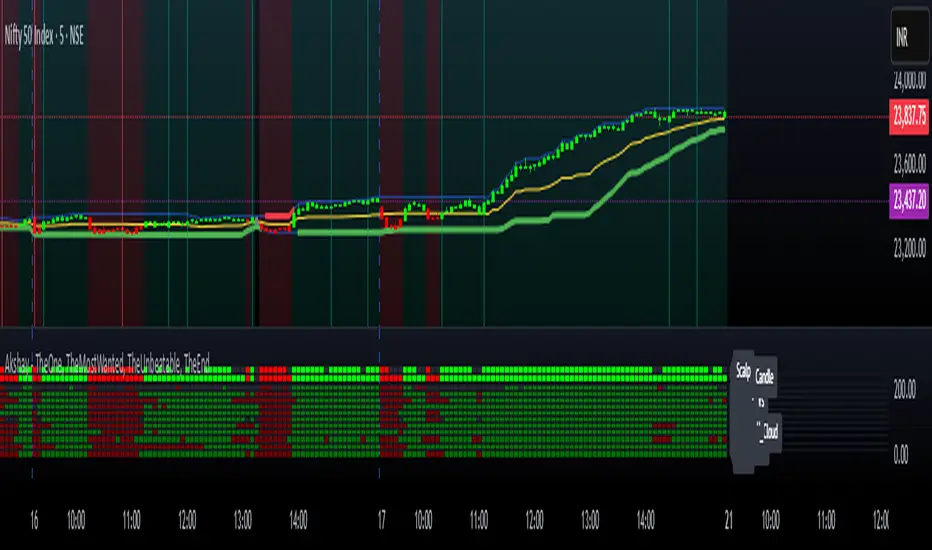
Akshay - TheOne, TheMostWanted, TheUnbeatable, TheEnd➤ All-in-One Solution (❌ No repaint):
This Technical Chart contains, MA24 Condition, Supertrend Indicator, HalfTrend Signal, Ichimoku Cloud Status, Parabolic SAR (P_SAR), First 5-Minute Candle Analysis (ORB5min), Volume-Weighted Moving Average (VWMA), Price-Volume Trend (PVT), Oscillator Composite, RSI Condition, ADX & Trend Strength.
Technicals don't lie.
🚀 Overview and Key Features
Comprehensive Multi-Indicator Approach:
The script is built to be an all-in-one technical indicator on TradingView. It integrates several well-known indicators and overlays—including Supertrend, HalfTrend, Ichimoku Cloud, various moving averages (EMA, SMA, VWMA), oscillators (Klinger, Price Oscillator, Awesome Oscillator, Chaikin Oscillator, Ultimate Oscillator, SMI Ergodic Oscillator, Chande Momentum Oscillator, Detrended Price Oscillator, Money Flow Index), ADX, and Donchian Channels—to create a composite picture of market sentiment.
Signal Generation and Alerts:
It not only calculates these indicators but also aggregates their output into “Master Candle” signals. Vertical lines are drawn on the chart with corresponding alerts to indicate potential buy or sell opportunities based on robust, combined conditions.
Visual Layering:
Through the use of colored histograms, custom candle plots, trend lines, and background color changes, the script offers a multi-layered visual representation of data, providing clarity about both short-term signals and overall market trends.
⚙️ How It Works and Functionality
MA24 Condition:
Uses the 24-period moving average as a proxy; if the price is above it, the bar is colored green, and red if below, with neutrality when conditions aren’t met.
Supertrend Indicator:
Evaluates price relative to the Supertrend level (calculated via ATR), coloring green when price is above it and red when below.
HalfTrend Signal:
Determines trend shifts by comparing the current close to a calculated trend level; green indicates an upward trend, while red suggests a downtrend.
Ichimoku Cloud Status:
Analyzes the relationship between the Conversion and Base lines; a bullish (green) signal is given when price is above both or the Conversion line is higher than the Base line.
Parabolic SAR (P_SAR):
Colors the signal based on whether the current price is above (green) or below (red) the Parabolic SAR marker, indicating stop and reverse conditions.
First 5-Minute Candle Analysis (ORB5min):
Uses key levels from the first 5-minute candle; if price exceeds the candle’s low, VWAP, and MA, it’s bullish (green), otherwise bearish (red).
Volume-Weighted Moving Average (VWMA):
Compares the current price to volume-weighted averages; a price above these levels is shown in green, below in red.
Price-Volume Trend (PVT):
Determines bullish or bearish momentum by comparing PVT to its VWAP—green when above and red when below.
Oscillator Composite:
Aggregates signals from multiple oscillators; a majority of positive results turn it green, while negative dominance results in red.
RSI Condition:
Uses a simple RSI threshold of 50, with values above signifying bullish (green) momentum and below marking bearish (red) conditions.
ADX & Trend Strength:
Reflects overall trend strength through ADX and directional movements; a combination favoring bullish conditions colors it green, with red signaling bearish pressure.
Master Candle Overall Signal:
Combines multiple indicator outputs into one “Master” signal—green for a consensus bullish trend and red for a bearish outlook.
Scalp Signal Variation:
Focused on short-term price changes, this signal adjusts quickly; green indicates improving short-term conditions, while red signals a downturn.
📊 Visualizations and 🎨 User Experience (❌ no repaint)
Dynamic Histograms & Bar Plots:
Each indicator is represented as a colored bar (with added vertical offsets) to facilitate easy comparison of their respective bullish or bearish contributions.
Clear Color-Coding & Labels:
Green (e.g., GreenFluorescent) indicates bullish sentiment.
Red (e.g., RedFluorescent) indicates bearish sentiment.
Custom labels and descriptive text accompany each bar for clarity.
Interactive Charting:
The overall background color adapts based on the “Master Candle” condition, offering an instant read on market sentiment.
The current candlestick is overlaid with color cues to reinforce the indicator’s signal, enhancing the trading experience.
Real-Time Alerts:
Vertical lines appear on signal events (buy/sell triggers), complemented by alerts that help traders stay on top of actionable market moves.
Sharp lines:
The Sharp lines are plotted based upon the EMA5 cross over with the same market trend, marks this as good time to reentry.
🔧 Settings and Customization
Flexible Timeframe Input:
Users can select their preferred timeframe for analysis, making the indicator adaptable to intraday or longer-term trading styles.
Customizable Indicator Parameters:
➤ Supertrend: Adjust ATR length and multiplier factors.
➤ HalfTrend: Tweak amplitude and channel deviation settings.
➤ Ichimoku Cloud & Oscillators: Fine-tune the conversion/base lines and oscillator lengths to match individual trading strategies.
Visual Customization:
The script’s color schemes and plotting styles can be altered as needed, giving users the freedom to tailor the interface to their taste or existing chart setups.
🌟 Uniqueness of the Concept
Integrated Multi-Indicator Synergy:
Combines a diverse range of trend, momentum, and volume-based indicators into a single cohesive system for a holistic market view.
Master Candle Aggregation:
Consolidates numerous individual signals into a "Master Candle" that filters out noise and provides a clear, consensus-based trading signal.
Layered Visual Feedback:
Uses color-coded histograms, adaptive background cues, and dynamic overlays to deliver a visually intuitive guide to market sentiment at a glance.
Customization and Flexibility:
Offers adjustable parameters for each indicator, allowing users to tailor the system to fit diverse trading styles and market conditions.
✅ Conclusion:
Robust Trading Tool & Non-Repainting Reliability:
This versatile technical analysis tool computes an extensive range of indicators, aggregates them into a stable, non-repainting “Master Candle” signal, and maintains consistent, verifiable outputs on historical data.
Holistic Market Insight & Consistent Signal Generation:
By combining trend detection, momentum oscillators, and volume analysis, the indicator delivers a comprehensive snapshot of market conditions and generates dependable signals across varying timeframes.
User-Centric Design with Rich Visual Feedback:
Customizable settings, clear color-coded outputs, adaptive backgrounds, and real-time alerts work together to provide actionable, transparent feedback—enhancing the overall trading experience.
A Unique All-in-One Solution:
The integrated approach not only simplifies complex market dynamics into an easy-to-read visual guide but also empowers systematic traders with a powerful, adaptable asset for accurate decision-making.
❤️ Credits:
Pine Script™ User Manual
Supertrend
Ichimoku Cloud
Parabolic SAR
Price Volume Trend (PVT)
Average Directional Index (ADX)
Volume Oscillator
HalfTrend
Donchian Trend
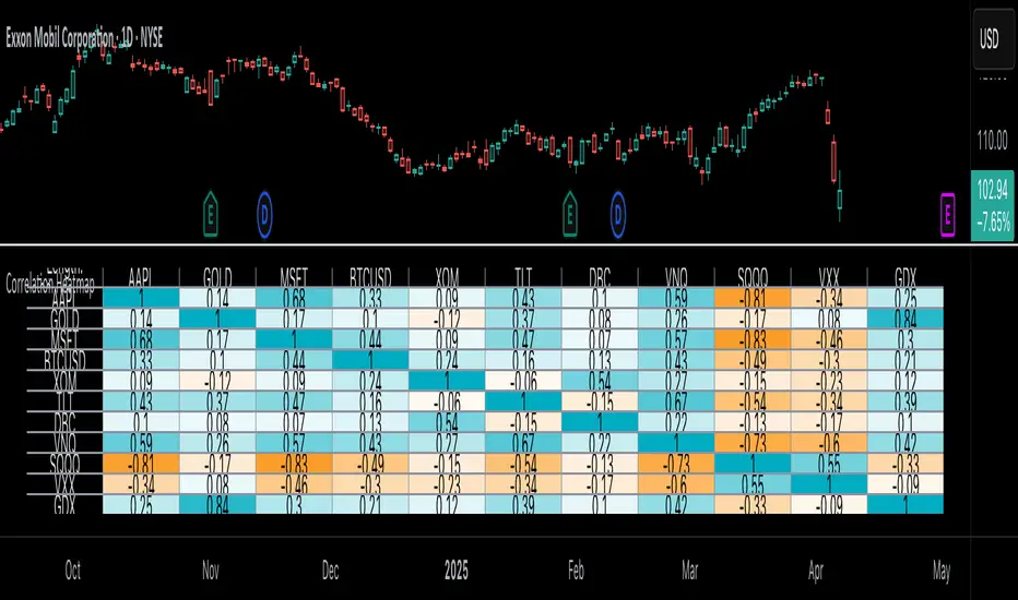
Correlation Heatmap█ OVERVIEW
This indicator creates a correlation matrix for a user-specified list of symbols based on their time-aligned weekly or monthly price returns. It calculates the Pearson correlation coefficient for each possible symbol pair, and it displays the results in a symmetric table with heatmap-colored cells. This format provides an intuitive view of the linear relationships between various symbols' price movements over a specific time range.
█ CONCEPTS
Correlation
Correlation typically refers to an observable statistical relationship between two datasets. In a financial time series context, it usually represents the extent to which sampled values from a pair of datasets, such as two series of price returns, vary jointly over time. More specifically, in this context, correlation describes the strength and direction of the relationship between the samples from both series.
If two separate time series tend to rise and fall together proportionally, they might be highly correlated. Likewise, if the series often vary in opposite directions, they might have a strong anticorrelation . If the two series do not exhibit a clear relationship, they might be uncorrelated .
Traders frequently analyze asset correlations to help optimize portfolios, assess market behaviors, identify potential risks, and support trading decisions. For instance, correlation often plays a key role in diversification . When two instruments exhibit a strong correlation in their returns, it might indicate that buying or selling both carries elevated unsystematic risk . Therefore, traders often aim to create balanced portfolios of relatively uncorrelated or anticorrelated assets to help promote investment diversity and potentially offset some of the risks.
When using correlation analysis to support investment decisions, it is crucial to understand the following caveats:
• Correlation does not imply causation . Two assets might vary jointly over an analyzed range, resulting in high correlation or anticorrelation in their returns, but that does not indicate that either instrument directly influences the other. Joint variability between assets might occur because of shared sensitivities to external factors, such as interest rates or global sentiment, or it might be entirely coincidental. In other words, correlation does not provide sufficient information to identify cause-and-effect relationships.
• Correlation does not predict the future relationship between two assets. It only reflects the estimated strength and direction of the relationship between the current analyzed samples. Financial time series are ever-changing. A strong trend between two assets can weaken or reverse in the future.
Correlation coefficient
A correlation coefficient is a numeric measure of correlation. Several coefficients exist, each quantifying different types of relationships between two datasets. The most common and widely known measure is the Pearson product-moment correlation coefficient , also known as the Pearson correlation coefficient or Pearson's r . Usually, when the term "correlation coefficient" is used without context, it refers to this correlation measure.
The Pearson correlation coefficient quantifies the strength and direction of the linear relationship between two variables. In other words, it indicates how consistently variables' values move together or in opposite directions in a proportional, linear manner. Its formula is as follows:
𝑟(𝑥, 𝑦) = cov(𝑥, 𝑦) / (𝜎𝑥 * 𝜎𝑦)
Where:
• 𝑥 is the first variable, and 𝑦 is the second variable.
• cov(𝑥, 𝑦) is the covariance between 𝑥 and 𝑦.
• 𝜎𝑥 is the standard deviation of 𝑥.
• 𝜎𝑦 is the standard deviation of 𝑦.
In essence, the correlation coefficient measures the covariance between two variables, normalized by the product of their standard deviations. The coefficient's value ranges from -1 to 1, allowing a more straightforward interpretation of the relationship between two datasets than what covariance alone provides:
• A value of 1 indicates a perfect positive correlation over the analyzed sample. As one variable's value changes, the other variable's value changes proportionally in the same direction .
• A value of -1 indicates a perfect negative correlation (anticorrelation). As one variable's value increases, the other variable's value decreases proportionally.
• A value of 0 indicates no linear relationship between the variables over the analyzed sample.
Aligning returns across instruments
In a financial time series, each data point (i.e., bar) in a sample represents information collected in periodic intervals. For instance, on a "1D" chart, bars form at specific times as successive days elapse.
However, the times of the data points for a symbol's standard dataset depend on its active sessions , and sessions vary across instrument types. For example, the daily session for NYSE stocks is 09:30 - 16:00 UTC-4/-5 on weekdays, Forex instruments have 24-hour sessions that span from 17:00 UTC-4/-5 on one weekday to 17:00 on the next, and new daily sessions for cryptocurrencies start at 00:00 UTC every day because crypto markets are consistently open.
Therefore, comparing the standard datasets for different asset types to identify correlations presents a challenge. If two symbols' datasets have bars that form at unaligned times, their correlation coefficient does not accurately describe their relationship. When calculating correlations between the returns for two assets, both datasets must maintain consistent time alignment in their values and cover identical ranges for meaningful results.
To address the issue of time alignment across instruments, this indicator requests confirmed weekly or monthly data from spread tickers constructed from the chart's ticker and another specified ticker. The datasets for spreads are derived from lower-timeframe data to ensure the values from all symbols come from aligned points in time, allowing a fair comparison between different instrument types. Additionally, each spread ticker ID includes necessary modifiers, such as extended hours and adjustments.
In this indicator, we use the following process to retrieve time-aligned returns for correlation calculations:
1. Request the current and previous prices from a spread representing the sum of the chart symbol and another symbol ( "chartSymbol + anotherSymbol" ).
2. Request the prices from another spread representing the difference between the two symbols ( "chartSymbol - anotherSymbol" ).
3. Calculate half of the difference between the values from both spreads ( 0.5 * (requestedSum - requestedDifference) ). The results represent the symbol's prices at times aligned with the sample points on the current chart.
4. Calculate the arithmetic return of the retrieved prices: (currentPrice - previousPrice) / previousPrice
5. Repeat steps 1-4 for each symbol requiring analysis.
It's crucial to note that because this process retrieves prices for a symbol at times consistent with periodic points on the current chart, the values can represent prices from before or after the closing time of the symbol's usual session.
Additionally, note that the maximum number of weeks or months in the correlation calculations depends on the chart's range and the largest time range common to all the requested symbols. To maximize the amount of data available for the calculations, we recommend setting the chart to use a daily or higher timeframe and specifying a chart symbol that covers a sufficient time range for your needs.
█ FEATURES
This indicator analyzes the correlations between several pairs of user-specified symbols to provide a structured, intuitive view of the relationships in their returns. Below are the indicator's key features:
Requesting a list of securities
The "Symbol list" text box in the indicator's "Settings/Inputs" tab accepts a comma-separated list of symbols or ticker identifiers with optional spaces (e.g., "XOM, MSFT, BITSTAMP:BTCUSD"). The indicator dynamically requests returns for each symbol in the list, then calculates the correlation between each pair of return series for its heatmap display.
Each item in the list must represent a valid symbol or ticker ID. If the list includes an invalid symbol, the script raises a runtime error.
To specify a broker/exchange for a symbol, include its name as a prefix with a colon in the "EXCHANGE:SYMBOL" format. If a symbol in the list does not specify an exchange prefix, the indicator selects the most commonly used exchange when requesting the data.
Note that the number of symbols allowed in the list depends on the user's plan. Users with non-professional plans can compare up to 20 symbols with this indicator, and users with professional plans can compare up to 32 symbols.
Timeframe and data length selection
The "Returns timeframe" input specifies whether the indicator uses weekly or monthly returns in its calculations. By default, its value is "1M", meaning the indicator analyzes monthly returns. Note that this script requires a chart timeframe lower than or equal to "1M". If the chart uses a higher timeframe, it causes a runtime error.
To customize the length of the data used in the correlation calculations, use the "Max periods" input. When enabled, the indicator limits the calculation window to the number of periods specified in the input field. Otherwise, it uses the chart's time range as the limit. The top-left corner of the table shows the number of confirmed weeks or months used in the calculations.
It's important to note that the number of confirmed periods in the correlation calculations is limited to the largest time range common to all the requested datasets, because a meaningful correlation matrix requires analyzing each symbol's returns under the same market conditions. Therefore, the correlation matrix can show different results for the same symbol pair if another listed symbol restricts the aligned data to a shorter time range.
Heatmap display
This indicator displays the correlations for each symbol pair in a heatmap-styled table representing a symmetric correlation matrix. Each row and column corresponds to a specific symbol, and the cells at their intersections correspond to symbol pairs . For example, the cell at the "AAPL" row and "MSFT" column shows the weekly or monthly correlation between those two symbols' returns. Likewise, the cell at the "MSFT" row and "AAPL" column shows the same value.
Note that the main diagonal cells in the display, where the row and column refer to the same symbol, all show a value of 1 because any series of non-na data is always perfectly correlated with itself.
The background of each correlation cell uses a gradient color based on the correlation value. By default, the gradient uses blue hues for positive correlation, orange hues for negative correlation, and white for no correlation. The intensity of each blue or orange hue corresponds to the strength of the measured correlation or anticorrelation. Users can customize the gradient's base colors using the inputs in the "Color gradient" section of the "Settings/Inputs" tab.
█ FOR Pine Script® CODERS
• This script uses the `getArrayFromString()` function from our ValueAtTime library to process the input list of symbols. The function splits the "string" value by its commas, then constructs an array of non-empty strings without leading or trailing whitespaces. Additionally, it uses the str.upper() function to convert each symbol's characters to uppercase.
• The script's `getAlignedReturns()` function requests time-aligned prices with two request.security() calls that use spread tickers based on the chart's symbol and another symbol. Then, it calculates the arithmetic return using the `changePercent()` function from the ta library. The `collectReturns()` function uses `getAlignedReturns()` within a loop and stores the data from each call within a matrix . The script calls the `arrayCorrelation()` function on pairs of rows from the returned matrix to calculate the correlation values.
• For consistency, the `getAlignedReturns()` function includes extended hours and dividend adjustment modifiers in its data requests. Additionally, it includes other settings inherited from the chart's context, such as "settlement-as-close" preferences.
• A Pine script can execute up to 40 or 64 unique `request.*()` function calls, depending on the user's plan. The maximum number of symbols this script compares is half the plan's limit, because `getAlignedReturns()` uses two request.security() calls.
• This script can use the request.security() function within a loop because all scripts in Pine v6 enable dynamic requests by default. Refer to the Dynamic requests section of the Other timeframes and data page to learn more about this feature, and see our v6 migration guide to learn what's new in Pine v6.
• The script's table uses two distinct color.from_gradient() calls in a switch structure to determine the cell colors for positive and negative correlation values. One call calculates the color for values from -1 to 0 based on the first and second input colors, and the other calculates the colors for values from 0 to 1 based on the second and third input colors.
Look first. Then leap.
ADR Nivele Horizontale dhe EMAThe user provided a Pine Script code for an indicator called "ADR Nivele Horizontale dhe EMA". The task is to explain how this code works. Hmm, first, I need to understand what this indicator does. The title mentions ADR levels and EMA, so it's probably combining horizontal lines based on Average Daily Range and some Exponential Moving Averages.
Looking at the code, the first part is the indicator declaration with version 6. The settings include an ADR period, levels above and below the mid, and line style. Then there's a section for calculations. They request daily high and low to compute the daily range. The ADR is the SMA of the daily range over the specified period. The mid is the average of daily high and low. The adr_val is half of ADR, maybe to create symmetrical levels around the mid.
Next, they create arrays for lines and labels above and below the mid. The loops go from 1 to levels_above/below, calculate each level, draw lines and labels. The mid line is also drawn with a different color. Then, there are several EMAs plotted: 13, 50, 200, 400, 600, 800, each with different colorsWait, but in Pine Script, when you use arrays to store lines and labels, you have to manage them properly to avoid repainting or memory issues. The code uses array.concat to add new lines and labels each bar. However, since this code is running on each bar, the for loops might be creating multiple lines each time, leading to too many objects. Oh right, but they use var to initialize the arrays, so they are only initialized once. Wait, no. The var keyword initializes the variable once, but in each iteration, they are concatenating new lines. Wait, no: the for loops are inside the main script, which runs on each bar. So every time a new bar is processed, the loops will run again, adding new lines and labels. That's a problem because each bar would create new lines, leading to an ever-increasing number of lines, which could hit the maximum limit (max_lines_count is set to 20, but maybe they have more bars). Oh, the indicator has max_lines_count=20, but the code might be creating multiple lines per bar. So maybe the code isn't handling the line management correctly. For example, if levels_above is 2, then each bar would create 2 new lines above and 2 below, plus the mid line. Over 20 bars, that's way over 20 lines. So this could cause the indicator to stop drawing after 20 lines. The user might not have realized that the lines are being recreated every bar, leading to a buildup. But perhaps the original code intended to have the lines update each bar, extending to the current bar. Let's see: in line.new, they use bar_index as the starting x1 and bar_index as x2. So each line is drawn from the previous bar's index to the current one. But since this is done on every bar, each line is only one bar long. Wait, no. Because on each new bar, the code creates a new line from the previous bar's index (bar_index , which is now the bar before the current one) to the current bar_index. So each line is just a segment from the previous bar to the current bar. But when the next bar comes, a new line is created again. So the result is that each level line is a series of one-bar-length segments, which might not be intended. The user probably wants continuous lines that extend from the left to the right, not just per bar. So this approach is incorrect. The correct way would be to have a line that starts at the first bar of the calculation and extends to the right, updating each bar. But the current code creates a new line each bar, leading to multiple short lines instead of one continuous line. That's a mistake.
So the main issue here is that the code is generating a new line segment for each bar, which is not efficient and would quickly hit the line limit. To fix this, instead of creating a new line every bar, they should create the line once and then update its position each bar. But in Pine Script, you can't directly update a line after it's created; instead, you need to track the line ID and use line.set_xy() to extend it. However, the current code uses array.concat to add new lines each bar, which isn't the right approach.
Therefore, the code as written will create multiple short lines instead of continuous horizontal lines. The correct approach for horizontal levels that extend to the right is to create the line once, starting at a certain bar and extending indefinitely, or to update the line's end point each new bar. But in Pine Script, you can't extend lines infinitely; you have to manage them each bar. Alternatively, using the 'line.extend' style might help, but I think the original code's logic is flawed here.
Additionally, the EMA part is straightforward: plotting multiple EMAs with different periods. That part should work as expected.
So the explanation should mention that the ADR levels are calculated based on the daily high and low, then the code attempts to draw horizontal lines above and below the mid-point. However, the way the lines are drawn may lead to multiple short segments instead of continuous lines, potentially causing performance issues or hitting the maximum line count. The EMAs are plotted correctly with various periods..

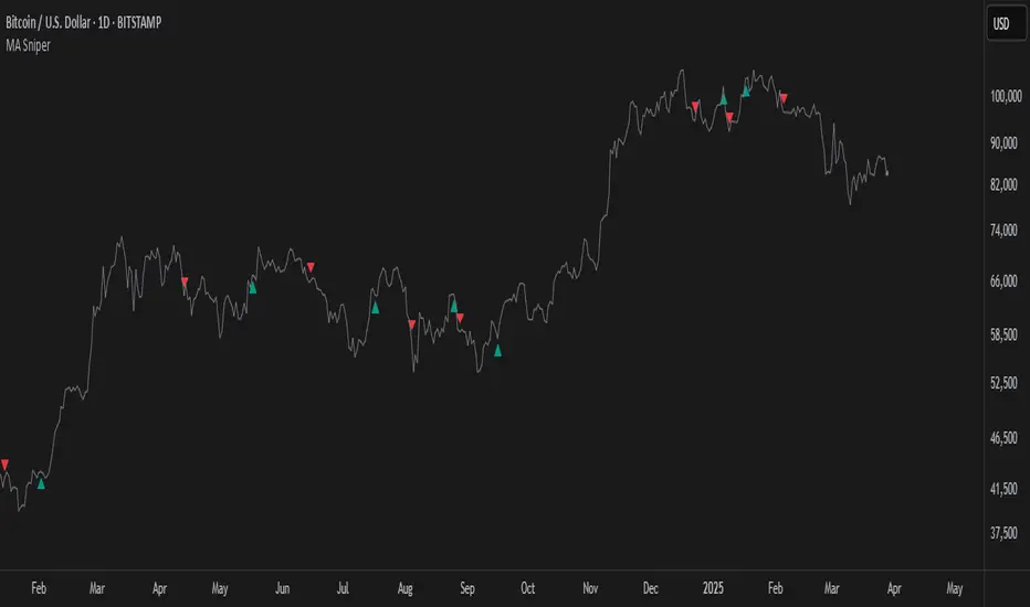
MA SniperThis indicator automatically finds the most effective moving average to use in a price crossover strategy—so you can focus on trading, not testing. It continuously evaluates a wide range of moving average periods, ranks them based on real-time market performance, and selects the one delivering the highest quality signals. The result? A smarter, adaptive tool that shows you exactly when price crosses its optimal moving average—bullish signals in green, bearish in red.
What makes it unique is the way it thinks.
Under the hood, the script doesn’t just pick a random MA or let you choose one manually. Instead, it backtests a large panel of moving average lengths for the current asset and timeframe. It evaluates each one by calculating its **Profit Factor**—a key performance metric used by pros to measure the quality of a strategy. Then, it assigns each MA a score and ranks them in a clean, built-in table so you can see, at a glance, which ones are currently most effective.
From that list, it picks the top-performing MA and uses it to generate live crossover signals on your chart. That MA is plotted automatically, and the signals adapt in real-time. This isn’t a static setup—it’s a dynamic system that evolves as the market evolves.
Even better: the indicator detects the type of instrument you’re trading (forex, stocks, etc.) and adjusts its internal calculations accordingly, including how many bars per day to consider. That means it remains highly accurate whether you’re trading EURUSD, SPX500, or TSLA.
You also get a real-time dashboard (via the table) that acts as a transparent scorecard. Want to see how other MAs are doing? You can. Want to understand why a certain MA was selected? The data is right there.
This tool is for traders who love crossover strategies but want something smarter, faster, and more precise—without spending hours manually testing. Whether you're scalping or swing trading, it offers a data-driven edge that’s hard to ignore.
Give it a try—you’ll quickly see how powerful it can be when your MA does the thinking for you.
This tool is for informational and educational purposes only. Trading involves risk, and past performance does not guarantee future results. Use responsibly.
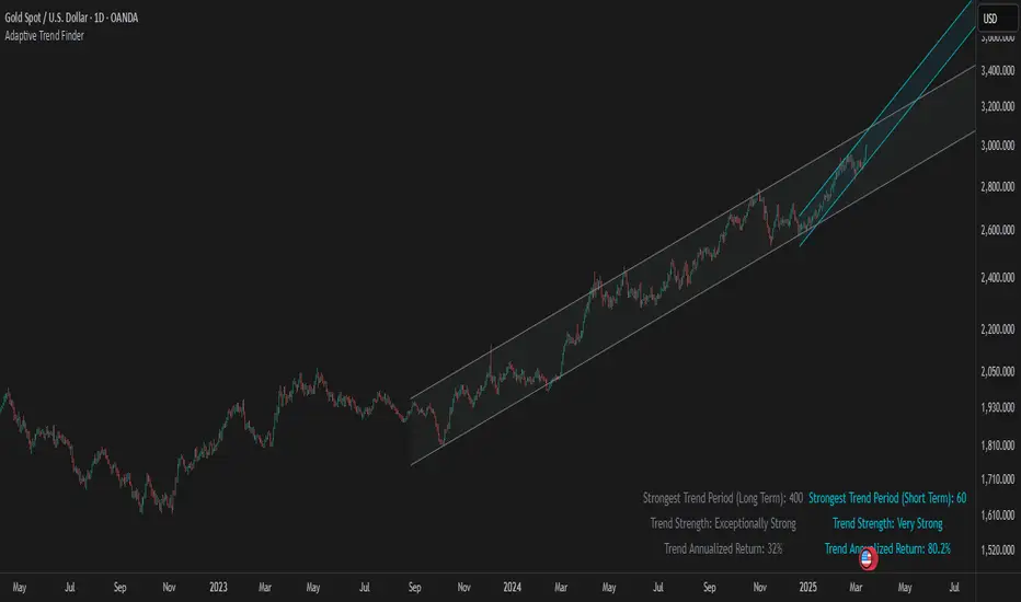
Adaptive Trend FinderAdaptive Trend Finder - The Ultimate Trend Detection Tool
Introducing Adaptive Trend Finder, the next evolution of trend analysis on TradingView. This powerful indicator is an enhanced and refined version of Adaptive Trend Finder (Log), designed to offer even greater flexibility, accuracy, and ease of use.
What’s New?
Unlike the previous version, Adaptive Trend Finder allows users to fully configure and adjust settings directly within the indicator menu, eliminating the need to modify chart settings manually. A major improvement is that users no longer need to adjust the chart's logarithmic scale manually in the chart settings; this can now be done directly within the indicator options, ensuring a smoother and more efficient experience. This makes it easier to switch between linear and logarithmic scaling without disrupting the analysis. This provides a seamless user experience where traders can instantly adapt the indicator to their needs without extra steps.
One of the most significant improvements is the complete code overhaul, which now enables simultaneous visualization of both long-term and short-term trend channels without needing to add the indicator twice. This not only improves workflow efficiency but also enhances chart readability by allowing traders to monitor multiple trend perspectives at once.
The interface has been entirely redesigned for a more intuitive user experience. Menus are now clearer, better structured, and offer more customization options, making it easier than ever to fine-tune the indicator to fit any trading strategy.
Key Features & Benefits
Automatic Trend Period Selection: The indicator dynamically identifies and applies the strongest trend period, ensuring optimal trend detection with no manual adjustments required. By analyzing historical price correlations, it selects the most statistically relevant trend duration automatically.
Dual Channel Display: Traders can view both long-term and short-term trend channels simultaneously, offering a broader perspective of market movements. This feature eliminates the need to apply the indicator twice, reducing screen clutter and improving efficiency.
Fully Adjustable Settings: Users can customize trend detection parameters directly within the indicator settings. No more switching chart settings – everything is accessible in one place.
Trend Strength & Confidence Metrics: The indicator calculates and displays a confidence score for each detected trend using Pearson correlation values. This helps traders gauge the reliability of a given trend before making decisions.
Midline & Channel Transparency Options: Users can fine-tune the visibility of trend channels, adjusting transparency levels to fit their personal charting style without overwhelming the price chart.
Annualized Return Calculation: For daily and weekly timeframes, the indicator provides an estimate of the trend’s performance over a year, helping traders evaluate potential long-term profitability.
Logarithmic Adjustment Support: Adaptive Trend Finder is compatible with both logarithmic and linear charts. Traders who analyze assets like cryptocurrencies, where log scaling is common, can enable this feature to refine trend calculations.
Intuitive & User-Friendly Interface: The updated menu structure is designed for ease of use, allowing quick and efficient modifications to settings, reducing the learning curve for new users.
Why is this the Best Trend Indicator?
Adaptive Trend Finder stands out as one of the most advanced trend analysis tools available on TradingView. Unlike conventional trend indicators, which rely on fixed parameters or lagging signals, Adaptive Trend Finder dynamically adjusts its settings based on real-time market conditions. By combining automatic trend detection, dual-channel visualization, real-time performance metrics, and an intuitive user interface, this indicator offers an unparalleled edge in trend identification and trading decision-making.
Traders no longer have to rely on guesswork or manually tweak settings to identify trends. Adaptive Trend Finder does the heavy lifting, ensuring that users are always working with the strongest and most reliable trends. The ability to simultaneously display both short-term and long-term trends allows for a more comprehensive market overview, making it ideal for scalpers, swing traders, and long-term investors alike.
With its state-of-the-art algorithms, fully customizable interface, and professional-grade accuracy, Adaptive Trend Finder is undoubtedly one of the most powerful trend indicators available.
Try it today and experience the future of trend analysis.
This indicator is a technical analysis tool designed to assist traders in identifying trends. It does not guarantee future performance or profitability. Users should conduct their own research and apply proper risk management before making trading decisions.
// Created by Julien Eche - @Julien_Eche
[GYTS-CE] Market Regime Detector🧊 Market Regime Detector (Community Edition)
🌸 Part of GoemonYae Trading System (GYTS) 🌸
🌸 --------- INTRODUCTION --------- 🌸
💮 What is the Market Regime Detector?
The Market Regime Detector is an advanced, consensus-based indicator that identifies the current market state to increase the probability of profitable trades. By distinguishing between trending (bullish or bearish) and cyclic (range-bound) market conditions, this detector helps you select appropriate tactics for different environments. Instead of forcing a single strategy across all market conditions, our detector allows you to adapt your approach based on real-time market behaviour.
💮 The Importance of Market Regimes
Markets constantly shift between different behavioural states or "regimes":
• Bullish trending markets - characterised by sustained upward price movement
• Bearish trending markets - characterised by sustained downward price movement
• Cyclic markets - characterised by range-bound, oscillating behaviour
Each regime requires fundamentally different trading approaches. Trend-following strategies excel in trending markets but fail in cyclic ones, while mean-reversion strategies shine in cyclic markets but underperform in trending conditions. Detecting these regimes is essential for successful trading, which is why we've developed the Market Regime Detector to accurately identify market states using complementary detection methods.
🌸 --------- KEY FEATURES --------- 🌸
💮 Consensus-Based Detection
Rather than relying on a single method, our detector employs two complementary detection methodologies that analyse different aspects of market behaviour:
• Dominant Cycle Average (DCA) - analyzes price movement relative to its lookback period, a proxy for the dominant cycle
• Volatility Channel - examines price behaviour within adaptive volatility bands
These diverse perspectives are synthesised into a robust consensus that minimises false signals while maintaining responsiveness to genuine regime changes.
💮 Dominant Cycle Framework
The Market Regime Detector uses the concept of dominant cycles to establish a reference framework. You can input the dominant cycle period that best represents the natural rhythm of your market, providing a stable foundation for regime detection across different timeframes.
💮 Intuitive Parameter System
We've distilled complex technical parameters into intuitive controls that traders can easily understand:
• Adaptability - how quickly the detector responds to changing market conditions
• Sensitivity - how readily the detector identifies transitions between regimes
• Consensus requirement - how much agreement is needed among detection methods
This approach makes the detector accessible to traders of all experience levels while preserving the power of the underlying algorithms.
💮 Visual Market Feedback
The detector provides clear visual feedback about the current market regime through:
• Colour-coded chart backgrounds (purple shades for bullish, pink for bearish, yellow for cyclic)
• Colour-coded price bars
• Strength indicators showing the degree of consensus
• Customizable colour schemes to match your preferences or trading system
💮 Integration in the GYTS suite
The Market Regime Detector is compatible with the GYTS Suite , i.e. it passes the regime into the 🎼 Order Orchestrator where you can set how to trade the trending and cyclic regime.
🌸 --------- CONFIGURATION SETTINGS --------- 🌸
💮 Adaptability
Controls how quickly the Market Regime detector adapts to changing market conditions. You can see it as a low-frequency, long-term change parameter:
Very Low: Very slow adaptation, most stable but may miss regime changes
Low: Slower adaptation, more stability but less responsiveness
Normal: Balanced between stability and responsiveness
High: Faster adaptation, more responsive but less stable
Very High: Very fast adaptation, highly responsive but may generate false signals
This setting affects lookback periods and filter parameters across all detection methods.
💮 Sensitivity
Controls how sensitive the detector is to market regime transitions. This acts as a high-frequency, short-term change parameter:
Very Low: Requires substantial evidence to identify a regime change
Low: Less sensitive, reduces false signals but may miss some transitions
Normal: Balanced sensitivity suitable for most markets
High: More sensitive, detects subtle regime changes but may have more noise
Very High: Very sensitive, detects minor fluctuations but may produce frequent changes
This setting affects thresholds for regime detection across all methods.
💮 Dominant Cycle Period
This parameter allows you to specify the market's natural rhythm in bars. This represents a complete market cycle (up and down movement). Finding the right value for your specific market and timeframe might require some experimentation, but it's a crucial parameter that helps the detector accurately identify regime changes. Most of the times the cycle is between 20 and 40 bars.
💮 Consensus Mode
Determines how the signals from both detection methods are combined to produce the final market regime:
• Any Method (OR) : Signals bullish/bearish if either method detects that regime. If methods conflict (one bullish, one bearish), the stronger signal wins. More sensitive, catches more regime changes but may produce more false signals.
• All Methods (AND) : Signals only when both methods agree on the regime. More conservative, reduces false signals but might miss some legitimate regime changes.
• Weighted Decision : Balances both methods with equal weighting. Provides a middle ground between sensitivity and stability.
Each mode also calculates a continuous regime strength value that's used for colour intensity in the 'unconstrained' display mode.
💮 Display Mode
Choose how to display the market regime colours:
• Unconstrained regime: Shows the regime strength as a continuous gradient. This provides more nuanced visualisation where the intensity of the colour indicates the strength of the trend.
• Consensus only: Shows only the final consensus regime with fixed colours based on the detected regime type.
The background and bar colours will change to indicate the current market regime:
• Purple shades: Bullish trending market (darker purple indicates stronger bullish trend)
• Pink shades: Bearish trending market (darker pink indicates stronger bearish trend)
• Yellow: Cyclic (range-bound) market
💮 Custom Colour Options
The Market Regime Detector allows you to customize the colour scheme to match your personal preferences or to coordinate with other indicators:
• Use custom colours: Toggle to enable your own colour choices instead of the default scheme
• Transparency: Adjust the transparency level of all regime colours
• Bullish colours: Define custom colours for strong, medium, weak, and very weak bullish trends
• Bearish colours: Define custom colours for strong, medium, weak, and very weak bearish trends
• Cyclic colour: Define a custom colour for cyclic (range-bound) market conditions
🌸 --------- DETECTION METHODS --------- 🌸
💮 Dominant Cycle Average (DCA)
The Dominant Cycle Average method forms a key part of our detection system:
1. Theoretical Foundation :
The DCA method builds on cycle analysis and the observation that in trending markets, price consistently remains on one side of a moving average calculated using the dominant cycle period. In contrast, during cyclic markets, price oscillates around this average.
2. Calculation Process :
• We calculate a Simple Moving Average (SMA) using the specified lookback period - a proxy for the dominant cycle period
• We then analyse the proportion of time that price spends above or below this SMA over a lookback window. The theory is that the price should cross the SMA each half cycle, assuming that the dominant cycle period is correct and price follows a sinusoid.
• This lookback window is adaptive, scaling with the dominant cycle period (controlled by the Adaptability setting)
• The different values are standardised and normalised to possess more resolving power and to be more robust to noise.
3. Regime Classification :
• When the normalised proportion exceeds a positive threshold (determined by Sensitivity setting), the market is classified as bullish trending
• When it falls below a negative threshold, the market is classified as bearish trending
• When the proportion remains between these thresholds, the market is classified as cyclic
💮 Volatility Channel
The Volatility Channel method complements the DCA method by focusing on price movement relative to adaptive volatility bands:
1. Theoretical Foundation :
This method is based on the observation that trending markets tend to sustain movement outside of normal volatility ranges, while cyclic markets tend to remain contained within these ranges. By creating adaptive bands that adjust to current market volatility, we can detect when price behaviour indicates a trending or cyclic regime.
2. Calculation Process :
• We first calculate a smooth base channel center using a low pass filter, creating a noise-reduced centreline for price
• True Range (TR) is used to measure market volatility, which is then smoothed and scaled by the deviation factor (controlled by Sensitivity)
• Upper and lower bands are created by adding and subtracting this scaled volatility from the centreline
• Price is smoothed using an adaptive A2RMA filter, which has a very flat and stable behaviour, to reduce noise while preserving trend characteristics
• The position of this smoothed price relative to the bands is continuously monitored
3. Regime Classification :
• When smoothed price moves above the upper band, the market is classified as bullish trending
• When smoothed price moves below the lower band, the market is classified as bearish trending
• When price remains between the bands, the market is classified as cyclic
• The magnitude of price's excursion beyond the bands is used to determine trend strength
4. Adaptive Behaviour :
• The smoothing periods and deviation calculations automatically adjust based on the Adaptability setting
• The measured volatility is calculated over a period proportional to the dominant cycle, ensuring the detector works across different timeframes
• Both the center line and the bands adapt dynamically to changing market conditions, making the detector responsive yet stable
This method provides a unique perspective that complements the DCA approach, with the consensus mechanism synthesising insights from both methods.
🌸 --------- USAGE GUIDE --------- 🌸
💮 Starting with Default Settings
The default settings (Normal for Adaptability and Sensitivity, Weighted Decision for Consensus Mode) provide a balanced starting point suitable for most markets and timeframes. Begin by observing how these settings identify regimes in your preferred instruments.
💮 Finding the Optimal Dominant Cycle
The dominant cycle period is a critical parameter. Here are some approaches to finding an appropriate value:
• Start with typical values, usually something around 25 works well
• Visually identify the average distance between significant peaks and troughs
• Experiment with different values and observe which provides the most stable regime identification
• Consider using cycle-finding indicators to help identify the natural rhythm of your market
💮 Adjusting Parameters
• If you notice too many regime changes → Decrease Sensitivity or increase Consensus requirement
• If regime changes seem delayed → Increase Adaptability
• If a trending regime is not detected, the market is automatically assigned to be in a cyclic state
• If you want to see more nuanced regime transitions → Try the "unconstrained" display mode (note that this will not affect the output to other indicators)
💮 Trading Applications
Regime-Specific Strategies:
• Bullish Trending Regime - Use trend-following strategies, trail stops wider, focus on breakouts, consider holding positions longer, and emphasize buying dips
• Bearish Trending Regime - Consider shorts, tighter stops, focus on breakdown points, sell rallies, implement downside protection, and reduce position sizes
• Cyclic Regime - Apply mean-reversion strategies, trade range boundaries, apply oscillators, target definable support/resistance levels, and use profit-taking at extremes
Strategy Switching:
Create a set of rules for each market regime and switch between them based on the detector's signal. This approach can significantly improve performance compared to applying a single strategy across all market conditions.
GYTS Suite Integration:
• In the GYTS 🎼 Order Orchestrator, select the '🔗 STREAM-int 🧊 Market Regime' as the market regime source
• Note that the consensus output (i.e. not the "unconstrained" display) will be used in this stream
• Create different strategies for trending (bullish/bearish) and cyclic regimes. The GYTS 🎼 Order Orchestrator is specifically made for this.
• The output stream is actually very simple, and can possibly be used in indicators and strategies as well. It outputs 1 for bullish, -1 for bearish and 0 for cyclic regime.
🌸 --------- FINAL NOTES --------- 🌸
💮 Development Philosophy
The Market Regime Detector has been developed with several key principles in mind:
1. Robustness - The detection methods have been rigorously tested across diverse markets and timeframes to ensure reliable performance.
2. Adaptability - The detector automatically adjusts to changing market conditions, requiring minimal manual intervention.
3. Complementarity - Each detection method provides a unique perspective, with the collective consensus being more reliable than any individual method.
4. Intuitiveness - Complex technical parameters have been abstracted into easily understood controls.
💮 Ongoing Refinement
The Market Regime Detector is under continuous development. We regularly:
• Fine-tune parameters based on expanded market data
• Research and integrate new detection methodologies
• Optimise computational efficiency for real-time analysis
Your feedback and suggestions are very important in this ongoing refinement process!
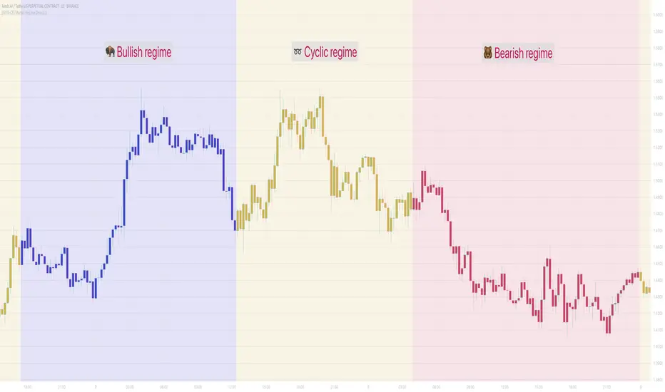
TimezoneLibrary with pre-defined timezone enums that can be used to request a timezone input from the user. The library provides a `tostring()` function to convert enum values to a valid string that can be used as a `timezone` parameter in pine script built-in functions. The library also includes a bonus function to get a formatted UTC offset from a UNIX timestamp.
The timezone enums in this library were compiled by referencing the available timezone options from TradingView chart settings as well as multiple Wikipedia articles relating to lists of time zones.
Some enums from this library are used to retrieve an IANA time zone identifier, while other enums only use UTC/GMT offset notation. It is important to note that the Pine Script User Manual recommends using IANA notation in most cases.
HOW TO USE
This library is intended to be used by Pine Coders who wish to provide their users with a simple way to input a timezone. Using this library is as easy as 1, 2, 3:
Step 1
Import the library into your script. Replace with the latest available version number for this library.
//@version=6
indicator("Example")
import n00btraders/Timezone/ as tz
Step 2
Select one of the available enums from the library and use it as an input. Tip: view the library source code and scroll through the enums at the top to find the best choice for your script.
timezoneInput = input.enum(tz.TimezoneID.EXCHANGE, "Timezone")
Step 3
Convert the user-selected input into a valid string that can be used in one of the pine script built-in functions that have a `timezone` parameter.
string timezone = tz.tostring(timezoneInput)
EXPORTED FUNCTIONS
There are multiple 𝚝𝚘𝚜𝚝𝚛𝚒𝚗𝚐() functions in this library: one for each timezone enum. The function takes a single parameter: any enum field from one of the available timezone enums that are exported by this library. Depending on the selected enum, the function will return a time zone string in either UTC/GMT notation or IANA notation.
Note: to avoid confusion with the built-in `str.tostring()` function, it is recommended to use this library's `tostring()` as a method rather than a function:
string timezone = timezoneInput.tostring()
offset(timestamp, format, timezone, prefix, colon)
Formats the time offset from a UNIX timestamp represented in a specified timezone.
Namespace types: series OffsetFormat
Parameters:
timestamp (int) : (series int) A UNIX time.
format (series OffsetFormat) : (series OffsetFormat) A time offset format.
timezone (string) : (series string) A UTC/GMT offset or IANA time zone identifier.
prefix (string) : (series string) Optional 'UTC' or 'GMT' prefix for the result.
colon (bool) : (series bool) Optional usage of colon separator.
Returns: Time zone offset using the selected format.
The 𝚘𝚏𝚏𝚜𝚎𝚝() function is provided as a convenient alternative to manually using `str.format_time()` and then manipulating the result.
The OffsetFormat enum is used to decide the format of the result from the `offset()` function. The library source code contains comments above this enum declaration that describe how each enum field will modify a time offset.
Tip: hover over the `offset()` function call in the Pine Editor to display a pop-up containing:
Function description
Detailed parameter list, including default values
Example function calls
Example outputs for different OffsetFormat.* enum values
NOTES
At the time of this publication, Pine cannot be used to access a chart's selected time zone. Therefore, the main benefit of this library is to provide a quick and easy way to create a pine script input for a time zone (most commonly, the same time zone selected in the user's chart settings).
At the time of the creation of this library, there are 95 Time Zones made available in the TradingView chart settings. If any changes are made to the time zone settings, this library will be updated to match the new changes.
All time zone enums (and their individual fields) in this library were manually verified and tested to ensure correctness.
An example usage of this library is included at the bottom of the source code.
Credits to HoanGhetti for providing a nice Markdown resource which I referenced to be able to create a formatted informational pop-up for this library's `offset()` function.

Uptrick: Time Based ReversionIntroduction
The Uptrick: Time Based Reversion indicator is designed to provide a comprehensive view of market momentum and potential trend shifts by combining multiple moving averages, a streak-based trend analysis system, and adaptive color visualization. It helps traders identify strong trends, spot potential reversals, and make more informed trading decisions.
Purpose
The primary goal of this indicator is to assist traders in distinguishing between sustained market movements and short-lived fluctuations. By evaluating how price behaves relative to its moving averages, and by measuring consecutive streaks above or below these averages, the indicator highlights areas where trends are likely to continue or lose momentum.
Overview
Uptrick: Time Based Reversion calculates one or more moving averages of price data and then tracks the number of consecutive bars (streaks) above or below these averages. This streak-based detection provides insight into whether a trend is gaining strength or nearing a potential reversal point. The indicator offers:
• Multiple moving average types (SMA, EMA, WMA)
• Optional second and third moving average layers for additional smoothing of first moving average
• A streak detection system to quantify trend intensity
• A dynamic color scheme that changes with streak strength
• Optional buy and sell signals for potential trade entries and exits
• A ribbon mode that applies moving averages to Open, High, Low, and Close prices for a more detailed visualization of overall trend alignment
Originality and Uniqueness
Unlike traditional moving average indicators, Uptrick: Time Based Reversion incorporates a streak measurement system to detect trend strength. This approach helps clarify whether a price movement is merely a quick fluctuation or part of a longer-lasting trend. Additionally, the optional ribbon mode extends this logic to Open, High, Low, and Close prices, creating a layered and intuitive visualization that shows complete trend alignment.
Inputs and Features
1. Enable Ribbon Mode
This input lets you activate or deactivate the ribbon display of multiple moving averages. When enabled, the script plots moving averages for the Open, High, Low, and Close prices and uses color fills to show whether these four data points are collectively above or below their respective moving averages.
2. Color Scheme Selection
Users can choose from several predefined color schemes, such as Default, Emerald, Crimson, Sapphire, Gold, Purple, Teal, Orange, Gray, Lime, or Aqua. Each scheme assigns distinct bullish, bearish and neutral colors..
3. Show Buy/Sell Signals
The indicator can display buy or sell signals based on its streak analysis logic. These signals appear as markers on the chart, indicating a “Safe Uptrend” (buy) or “Safe Downtrend” (sell).
4. Moving Average Types and Lengths
• First MA Type and Length: Choose SMA, EMA, or WMA along with a customizable period.
• Second and Third MA Types and Lengths: You can optionally stack additional moving averages for further smoothing, each with its own customizable type and period.
5. Streak Threshold Multiplier
This numeric input determines how strong a streak must be before the script considers it a “safe” trend. A higher multiplier requires a longer or more intense streak for a buy or sell signal.
6. Dynamic Transparency Calculation
The color intensity adapts to the streak’s strength. Longer streaks increase the transparency of the opposing color, making the current dominant color stand out. This feature ensures that a vigorous uptrend or downtrend is visually distinct from short-lived or weaker moves.
7. Ribbon Moving Averages
In ribbon mode, the script calculates moving averages for the Open, High, Low, and Close prices. Each of these is optionally smoothed again if the second and/or third moving average layers are active. The final result is a ribbon of moving averages that helps confirm whether the market is uniformly aligned above or below these key reference points.
Calculation Methodology
1. Initial Moving Average
The script calculates the first moving average (SMA, EMA, or WMA) of the closing price over a user-defined period.
2. Optional Secondary and Tertiary Averages
If selected, the script then applies a second and/or third smoothing step. Each of these steps can be a different type of moving average (SMA, EMA, or WMA) with its own period length.
3. Streak Detection
The indicator counts consecutive bars above or below the smoothed moving average. A running total (streakUp or streakDown) increments with every bar that remains above or below that average.
4. Reversion Intensity
The script compares the current streak value to its own average (calculated over the final chosen period). This ratio determines whether the streak is nearing a likely reversion or is strong enough to continue.
5. Color Assignment and Signals
The indicator calculates color transparency based on streak intensity. Buy and sell signals appear when the streak meets or exceeds the threshold multiplier, indicating a safe uptrend or downtrend.
Color Schemes and Visualization
This indicator offers multiple predefined color sets. Each scheme specifies a unique bullish color, bearish color and neutral color. The script automatically varies transparency to highlight strong trends and fade weaker ones, making it visually clear when a trend is intensifying or losing momentum.
Smoothing Techniques
By allowing up to three layers of moving average smoothing, the indicator accommodates different trading styles. A single layer provides faster reactions to market changes, while more layers reduce noise at the cost of slower responsiveness. Traders can choose the right balance between responsiveness and stability for their strategy, whether it is short-term scalping or long-term trend following.
Why It Combines Specific Smoothing Techniques
The Uptrick: Time Based Reversion indicator strategically combines specific smoothing techniques—SMA, EMA, and WMA—to leverage their complementary strengths. The SMA provides stable and consistent trend identification by equally weighting all data points, while the EMA emphasizes recent price movements, allowing quicker responses to market changes. WMA enhances sensitivity to recent price shifts, which helps in detecting subtle momentum changes early. By integrating these methods in layers, the indicator effectively balances responsiveness with stability, helping traders clearly identify genuine trend changes while filtering out short-term noise and false signals.
Ribbon Mode
If Open, High, Low, and Close prices remain above or below their respective moving averages consistently, the script colors the bars fully bullish or bearish. When the data points are mixed, a neutral color is applied. This mode provides a thorough perspective on whether the entire price range is aligned in one direction or showing conflicting signals.
Summary
Uptrick: Time Based Reversion combines multiple moving averages, streak detection, and dynamic color adjustments to help traders identify significant trends and potential reversal areas. Its flexibility allows it to be used either in a simpler form, with one moving average and streak analysis, or in a more advanced configuration with ribbon mode that charts multiple smoothed averages for a deeper understanding of price alignment. By adapting color intensities based on streak strength and providing optional buy/sell signals, this indicator delivers a clear and flexible tool suited to various trading strategies.
Disclaimer
This indicator is designed as an analysis aid and does not guarantee profitable trades. Past performance does not indicate future success, and market conditions can change unexpectedly. Users are advised to employ proper risk management and thoroughly evaluate trades before taking positions. Use this indicator as part of a broader strategy, not as a sole decision-making tool.
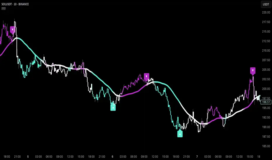
Normalised Price Crossover - MACD but TickersEver noticed two different tickers are correlated yet have different lags? Ever find one ticker moves first and when the other finally goes to catch up, the first one has already reversed?
So I thought to myself, would be wicked if I took the faster one and made it into a 'Signal Line' and the slow one and made it into a 'Slow Line' almost like a MACD if you will.
So that's what I did, I took the price charts of the tickers and I normalised the price data so they could actually cross, plotted it and sat back to see it generate signals, lo and behold!
Pretty neat, though I'd advise to use spreads and such for the different tickers to really feel the power of the indicator, works well when you use formulas that model actual mechanisms instead of arbitrary price data of different assets as correlation =/= causation.
Enjoy.

[TehThomas] - ICT Volume ImbalanceThis script is a Volume Imbalance (VI) detector and visualizer for use on the TradingView platform. The goal of the script is to automatically identify areas where there are significant imbalances in the volume of trades between consecutive candlesticks and visually highlight these areas. These imbalances can provide traders with valuable insights about the market’s current condition, often signaling potential reversal or continuation points based on price and volume action.
ICT (Inner Circle Trader) Concept of Volume Imbalances
Volume imbalances are a critical concept in the ICT trading methodology. They refer to situations where there is an unusual or significant difference in volume between two consecutive candlesticks, which might indicate institutional or large player activity. According to ICT principles, these imbalances can show us areas of market inefficiency or potential price manipulation. By identifying these imbalances, traders can gain an edge in understanding where the market is likely to move next.
Bullish and Bearish Volume Imbalances:
Bullish Volume Imbalance: This occurs when there is a strong increase in buying pressure, typically indicated by a higher volume on a candle that closes significantly above the previous one, often leaving a gap or larger price movement. The market could be preparing to push higher, and the volume shows a clear shift in buying demand.
Bearish Volume Imbalance:
Conversely, a bearish imbalance occurs when there is a strong increase in selling pressure, typically signaled by a candle that closes significantly lower than the previous one, again with higher volume. This could indicate that large players are offloading positions, and the price is likely to drop further.
Key Features and Functions of the Script
The script automates the process of detecting these volume imbalances and visually marking them on a price chart. Let’s explore its functionality in detail.
1. Inputs Section
The script allows for significant customization through its input options, which help traders adjust the detection and visualization of volume imbalances based on their individual preferences and trading style. Below are the details:
lookback (250 bars): This input specifies the number of bars (or candles) the script should look back when analyzing the volume imbalance. By setting this to 250, the user is looking at the last 250 bars on the chart to detect any significant volume imbalances. This period is adjustable between 50 to 500 bars.
volumeThreshold (1.0 multiplier): This input helps set the sensitivity for identifying volume imbalances. The script compares the volume of the current candle with the previous one, and if the current volume exceeds the previous volume by this threshold multiplier (in this case, 1.0 means at least equal to the previous volume), then it triggers an imbalance. Users can adjust the multiplier to suit different market conditions.
showBoxes (true/false): This toggle determines whether the boxes representing volume imbalances are drawn on the chart. When enabled, the script visually highlights the imbalances with colored boxes.
fillBaseColor (orange with 80% opacity): This is the color setting for the background of the imbalance boxes. A softer color (like orange with opacity) ensures the imbalance is highlighted without obscuring the price action.
borderColor (gray): The color of the border around the imbalance boxes. This adds a visual distinction to make the imbalance areas more visible.
borderWidth (1 pixel): This controls the width of the box's border to adjust how prominent it appears.
rightOffset (30 bars): This input controls how far the imbalance box extends to the right on the chart. It helps users anticipate the potential continuation of the imbalance beyond the current candle.
allowWickOverlap (true/false): This setting allows imbalances to be identified even if the wicks of the two consecutive candlesticks overlap. If set to false, only imbalances where the bodies of the candlesticks don’t overlap are considered.
showBrokenBoxes (true/false): If enabled, once a volume imbalance no longer holds true (i.e., the price breaks through the box), the box is marked as "broken." If disabled, the box is deleted when the imbalance condition no longer applies.
brokenBoxColor (red): This controls the color of the box when it is broken, which can be used as a visual cue that the imbalance was invalidated or no longer valid for analysis.
2. Volume Imbalance Function
This is the core function of the script, where the logic to detect bullish and bearish volume imbalances is implemented.
Bullish Imbalance Condition:
The first condition checks if the low of the current candle is greater than the high of the previous candle. This suggests that the market is moving upward with buying pressure.
The second condition checks whether the volume of the current candle is higher than the previous candle by the volumeThreshold multiplier. If both conditions are satisfied, a bullish imbalance is detected.
Bearish Imbalance Condition:
The first condition checks if the high of the current candle is lower than the low of the previous candle. This suggests downward price action with selling pressure.
The second condition checks whether the current volume exceeds the previous volume by the threshold
Allow Wick Overlap: If allowWickOverlap is set to true, the script will still detect imbalances if the wicks of the two candles overlap (common in volatile markets). If false, imbalances are only considered if the wicks do not overlap.
3. Box Creation and Management
When a volume imbalance is detected, the script creates a box on the chart:
The bullish imbalance box is drawn using the minimum of the open and close of the current bar as the top boundary and the maximum of the open and close of the previous bar as the bottom boundary.
Conversely, the bearish imbalance box is drawn in reverse, using the maximum of the current bar’s open and close as the top boundary and the minimum of the previous bar’s open and close as the bottom boundary.
Once the box is created, it is displayed on the chart with the specified background color, border color, and width.
4. Processing Existing Boxes
After detecting a new imbalance and drawing a box, the script checks whether the box should still remain on the chart:
If the price moves beyond the boundaries of the imbalance box, the box is marked as broken (if showBrokenBoxes is enabled), and its color is changed to red, signifying that the imbalance is no longer valid.
If the box remains intact (i.e., the price has not broken the defined boundaries), the script keeps the box extended to the right as the market continues to evolve.
5. Removing Outdated Boxes
Lastly, the script removes boxes that are older than the specified lookback period. For example, if a box was created 250 bars ago, it will be deleted after that period. This ensures the chart stays clean and only focuses on relevant imbalances.
Why This Script is Useful for Traders
This script is extremely valuable for traders, especially those following the ICT methodology, because it automates the process of detecting market inefficiencies or imbalances that might signal future price action. Here’s why it’s particularly useful:
Identifying Key Areas of Interest: Volume imbalances often point to areas where institutional or large-scale traders have entered the market. These areas could provide clues about the next significant move in the market.
Visualizing Market Structure: By automatically drawing boxes around volume imbalances, the script helps traders visually identify potential areas of support, resistance, or turning points, enabling them to make informed trading decisions.
Time Efficiency: Instead of manually analyzing each candlestick and volume spike, this script does the heavy lifting, saving traders valuable time and allowing them to focus on other aspects of their strategy.
Enhanced Trade Entries and Exits: By understanding where volume imbalances are occurring, traders can time their entries (buying during bullish imbalances and selling during bearish ones) and exits (as imbalances break) more effectively, thus improving their chances of success.
Conclusion
In summary, this script is a powerful tool for traders looking to implement volume imbalance strategies based on the ICT methodology. It automates the identification and visualization of significant imbalances in price and volume, offering traders a clear visual representation of potential market turning points. By customizing the settings, traders can tailor the script to their preferred timeframes and sensitivity, making it a flexible and effective tool for any trading strategy.
__________________________________________
Thanks for your support!
If you found this idea helpful or learned something new, drop a like 👍 and leave a comment, I’d love to hear your thoughts! 🚀
Make sure to follow me for more price action insights, free indicators, and trading guides. Let’s grow and trade smarter together! 📈
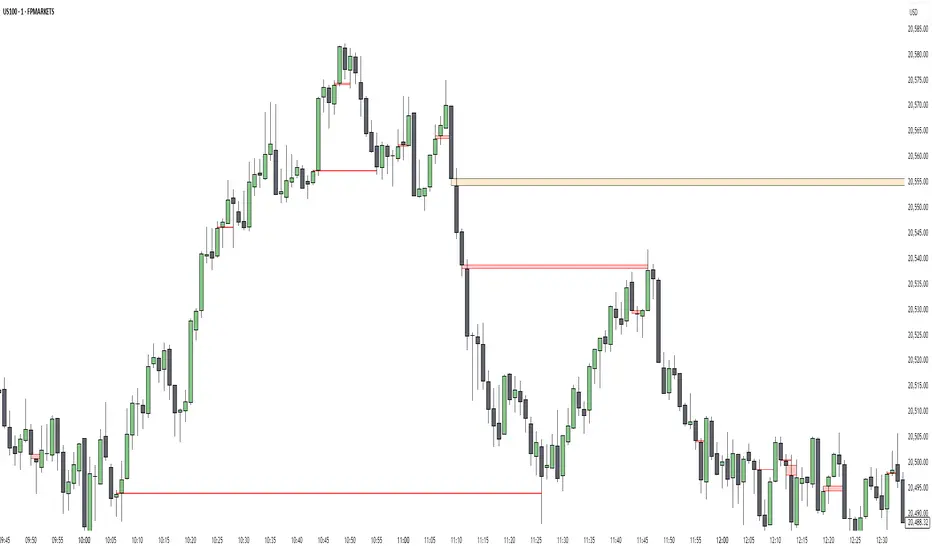
[COG]TMS Crossfire 🔍 TMS Crossfire: Guide to Parameters
📊 Core Parameters
🔸 Stochastic Settings (K, D, Period)
- **What it does**: These control how the first stochastic oscillator works. Think of it as measuring momentum speed.
- **K**: Determines how smooth the main stochastic line is. Lower values (1-3) react quickly, higher values (3-9) are smoother.
- **D**: Controls the smoothness of the signal line. Usually kept equal to or slightly higher than K.
- **Period**: How many candles are used to calculate the stochastic. Standard is 14 days, lower for faster signals.
- **For beginners**: Start with the defaults (K:3, D:3, Period:14) until you understand how they work.
🔸 Second Stochastic (K2, D2, Period2)
- **What it does**: Creates a second, independent stochastic for stronger confirmation.
- **How to use**: Can be set identical to the first one, or with slightly different values for dual confirmation.
- **For beginners**: Start with the same values as the first stochastic, then experiment.
🔸 RSI Length
- **What it does**: Controls the period for the RSI calculation, which measures buying/selling pressure.
- **Lower values** (7-9): More sensitive, good for short-term trading
- **Higher values** (14-21): More stable, better for swing trading
- **For beginners**: The default of 11 is a good balance between speed and reliability.
🔸 Cross Level
- **What it does**: The centerline where crosses generate signals (default is 50).
- **Traditional levels**: Stochastics typically use 20/80, but 50 works well for this combined indicator.
- **For beginners**: Keep at 50 to focus on trend following strategies.
🔸 Source
- **What it does**: Determines which price data is used for calculations.
- **Common options**:
- Close: Most common and reliable
- Open: Less common
- High/Low: Used for specialized indicators
- **For beginners**: Stick with "close" as it's most commonly used and reliable.
🎨 Visual Theme Settings
🔸 Bullish/Bearish Main
- **What it does**: Sets the overall color scheme for bullish (up) and bearish (down) movements.
- **For beginners**: Green for bullish and red for bearish is intuitive, but choose any colors that are easy for you to distinguish.
🔸 Bullish/Bearish Entry
- **What it does**: Colors for the entry signals shown directly on the chart.
- **For beginners**: Use bright, attention-grabbing colors that stand out from your chart background.
🌈 Line Colors
🔸 K1, K2, RSI (Bullish/Bearish)
- **What it does**: Controls the colors of each indicator line based on market direction.
- **For beginners**: Use different colors for each line so you can quickly identify which line is which.
⏱️ HTF (Higher Timeframe) Settings
🔸 HTF Timeframe
- **What it does**: Sets which higher timeframe to use for filtering (e.g., 240 = 4 hour chart).
- **How to choose**: Should be at least 4x your current chart timeframe (e.g., if trading on 15min, use 60min or higher).
- **For beginners**: Start with a timeframe 4x higher than your trading chart.
🔸 Use HTF Filter
- **What it does**: Toggles whether the higher timeframe filter is applied or not.
- **For beginners**: Keep enabled to reduce false signals, especially when learning.
🔸 HTF Confirmation Bars
- **What it does**: How many bars must confirm a trend change on higher timeframe.
- **Higher values**: More reliable but slower to react
- **Lower values**: Faster signals but more false positives
- **For beginners**: Start with 2-3 bars for a good balance.
📈 EMA Settings
🔸 Use EMA Filter
- **What it does**: Toggles price filtering with an Exponential Moving Average.
- **For beginners**: Keep enabled for better trend confirmation.
🔸 EMA Period
- **What it does**: Length of the EMA for filtering (shorter = faster reactions).
- **Common values**:
- 5-13: Short-term trends
- 21-50: Medium-term trends
- 100-200: Long-term trends
- **For beginners**: 5-10 is good for short-term trading, 21 for swing trading.
🔸 EMA Offset
- **What it does**: Shifts the EMA forward or backward on the chart.
- **For beginners**: Start with 0 and adjust only if needed for visual clarity.
🔸 Show EMA on Chart
- **What it does**: Toggles whether the EMA appears on your main price chart.
- **For beginners**: Keep enabled to see how price relates to the EMA.
🔸 EMA Color, Style, Width, Transparency
- **What it does**: Customizes how the EMA line looks on your chart.
- **For beginners**: Choose settings that make the EMA visible but not distracting.
🌊 Trend Filter Settings
🔸 Use EMA Trend Filter
- **What it does**: Enables a multi-EMA system that defines the overall market trend.
- **For beginners**: Keep enabled for stronger trend confirmation.
🔸 Show Trend EMAs
- **What it does**: Toggles visibility of the trend EMAs on your chart.
- **For beginners**: Enable to see how price moves relative to multiple EMAs.
🔸 EMA Line Thickness
- **What it does**: Controls how the thickness of EMA lines is determined.
- **Options**:
- Uniform: All EMAs have the same thickness
- Variable: Each EMA has its own custom thickness
- Hierarchical: Automatically sized based on period (longer periods = thicker)
- **For beginners**: "Hierarchical" is most intuitive as longer-term EMAs appear more dominant.
🔸 EMA Line Style
- **What it does**: Sets the line style (solid, dotted, dashed) for all EMAs.
- **For beginners**: "Solid" is usually clearest unless you have many lines overlapping.
🎭 Trend Filter Colors/Width
🔸 EMA Colors (8, 21, 34, 55)
- **What it does**: Sets the color for each individual trend EMA.
- **For beginners**: Use a logical progression (e.g., shorter EMAs brighter, longer EMAs darker).
🔸 EMA Width Settings
- **What it does**: Controls the thickness of each EMA line.
- **For beginners**: Thicker lines for longer EMAs make them easier to distinguish.
🔔 How These Parameters Work Together
The power of this indicator comes from how these components interact:
1. **Base Oscillator**: The stochastic and RSI components create the main oscillator
2. **HTF Filter**: The higher timeframe filter prevents trading against larger trends
3. **EMA Filter**: The EMA filter confirms signals with price action
4. **Trend System**: The multi-EMA system identifies the overall market environment
Think of it as multiple layers of confirmation, each adding more reliability to your trading signals.
💡 Tips for Beginners
1. **Start with defaults**: Use the default settings first and understand what each element does
2. **One change at a time**: When customizing, change only one parameter at a time
3. **Keep notes**: Write down how each change affects your results
4. **Backtest thoroughly**: Test any changes on historical data before trading real money
5. **Less is more**: Sometimes simpler settings work better than complicated ones
Remember, no indicator is perfect - always combine this with proper risk management and other forms of analysis!
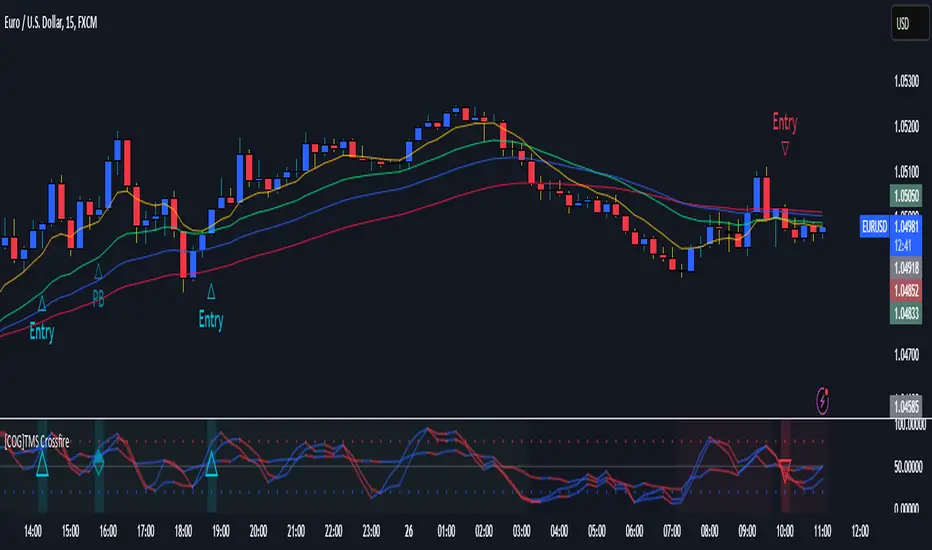
Uptrick: Alpha TrendIntroduction
Uptrick: Alpha Trend is a comprehensive technical analysis indicator designed to provide traders with detailed insights into market trends, momentum, and risk metrics. It adapts to various trading styles—from quick scalps to longer-term positions—by dynamically adjusting its calculations and visual elements. By combining multiple smoothing techniques, advanced color schemes, and customizable data tables, the indicator offers a holistic view of market behavior.
Originality
The Alpha Trend indicator distinguishes itself by blending established technical concepts with innovative adaptations. It employs three different smoothing techniques tailored to specific trading modes (Scalp, Swing, and Position), and it dynamically adjusts its parameters to match the chosen mode. The indicator also offers a wide range of color palettes and multiple on-screen tables that display key metrics. This unique combination of features, along with its ability to adapt in real time, sets it apart as a versatile tool for both novice and experienced traders.
Features
1. Multi-Mode Trend Line
The indicator automatically selects a smoothing method based on the trading mode:
- Scalp Mode uses the Hull Moving Average (HMA) for rapid responsiveness.
- Swing Mode employs the Exponential Moving Average (EMA) for balanced reactivity.
- Position Mode applies the Weighted Moving Average (WMA) for smoother, long-term trends.
Each method is chosen to best capture the price action dynamics appropriate to the trader’s timeframe.
2. Adaptive Momentum Thresholds
It tracks bullish and bearish momentum with counters that increment as the trend confirms directional movement. When these counters exceed a user-defined threshold, the indicator generates optional buy or sell signals. This approach helps filter out minor fluctuations and highlights significant market moves.
3. Gradient Fills
Two types of fills enhance visual clarity:
- Standard Gradient Fill displays ATR-based zones above and below the trend line, indicating potential bullish and bearish areas.
- Fading Gradient Fill creates a smooth transition between the trend line and the price, visually emphasizing the distance between them.
4. Bar Coloring and Signal Markers
The indicator can color-code bars based on market conditions—bullish, bearish, or neutral—allowing for immediate visual assessment. Additionally, signal markers such as buy and sell arrows are plotted when momentum thresholds are breached.
5. Comprehensive Data Tables
Uptrick: Alpha Trend offers several optional tables for detailed analysis:
- Insider Info: Displays key metrics like the current trend value, bullish/bearish momentum counts, and ATR.
- Indicator Metrics: Lists input settings such as trend length, damping, signal threshold, and net momentum.
- Market Analysis: Summarizes overall trend direction, trend strength, Sortino ratio, return, and volatility.
- Price & Trend Dynamics: Details price deviation from the trend, trend slope, and ATR ratio.
- Momentum & Volatility Insights: Presents RSI, standard deviation (volatility), and net momentum.
- Performance & Acceleration Metrics: Focuses on the Sortino ratio, trend acceleration, return, and trend strength.
Each table can be positioned flexibly on the chart, allowing traders to customize the layout according to their needs.
Why It Combines Specific Smoothing Techniques
Smoothing techniques are essential for filtering out market noise and revealing underlying trends. The indicator combines three smoothing methods for the following reasons:
- The Hull Moving Average (HMA) in Scalp Mode minimizes lag and responds quickly to price changes, which is critical for short-term trading.
- The Exponential Moving Average (EMA) in Swing Mode gives more weight to recent data, striking a balance between speed and smoothness. This makes it suitable for mid-term trend analysis.
- The Weighted Moving Average (WMA) in Position Mode smooths out short-term fluctuations, offering a clear view of longer-term trends and reducing the impact of transient market volatility.
By using these specific methods in their respective trading modes, the indicator ensures that the trend line is appropriately responsive for the intended time frame, enhancing decision-making while maintaining clarity.
Inputs
1. Trend Length (Default: 30)
Defines the lookback period for the smoothing calculation. A shorter trend length results in a more responsive line, while a longer length produces a smoother, less volatile trend.
2. Trend Damping (Default: 0.75)
Controls the degree of smoothing applied to the trend line. Lower values lead to a smoother curve, whereas higher values increase sensitivity to price fluctuations.
3. Signal Strength Threshold (Default: 5)
Specifies the number of consecutive bullish or bearish bars required to trigger a signal. Higher thresholds reduce the frequency of signals, focusing on stronger moves.
4. Enable Bar Coloring (Default: True)
Toggles whether each price bar is colored to indicate bullish, bearish, or neutral conditions.
5. Enable Signals (Default: True)
When enabled, this option plots buy or sell arrows on the chart once the momentum thresholds are met.
6. Enable Standard Gradient Fill (Default: False)
Activates ATR-based gradient fills around the trend line to visualize potential support and resistance zones.
7. Enable Fading Gradient Fill (Default: True)
Draws a gradual color transition between the trend line and the current price, emphasizing their divergence.
8. Trading Mode (Options: Scalp, Swing, Position)
Determines which smoothing method and ATR period to use, adapting the indicator’s behavior to short-term, medium-term, or long-term trading.
9. Table Position Inputs
Allows users to select from nine possible chart positions (top, middle, bottom; left, center, right) for each data table.
10. Show Table Booleans
Separate toggles control the display of each table (Insider Info, Indicator Metrics, Market Analysis, and the three Deep Tables), enabling a customized view of the data.
Color Schemes
(Default) - The colors in the preview image of the indicator.
(Emerald)
(Sapphire)
(Golden Blaze)
(Mystic)
(Monochrome)
(Pastel)
(Vibrant)
(Earth)
(Neon)
Calculations
1. Trend Line Methods
- Scalp Mode: Utilizes the Hull Moving Average (HMA), which computes two weighted moving averages (one at half the length and one at full length), subtracts them, and then applies a final weighted average based on the square root of the length. This method minimizes lag and increases responsiveness.
- Swing Mode: Uses the Exponential Moving Average (EMA), which assigns greater weight to recent prices, thus balancing quick reaction with smoothness.
- Position Mode: Applies the Weighted Moving Average (WMA) to focus on longer-term trends by emphasizing the entire lookback period and reducing the impact of short-term volatility.
2. Momentum Tracking
The indicator maintains separate counters for bullish and bearish momentum. These counters increase as the trend confirms directional movement and reset when the trend reverses. When a counter exceeds the defined signal strength threshold, a corresponding signal (buy or sell) is triggered.
3. Volatility and ATR Zones
The Average True Range (ATR) is calculated using a period that adapts to the selected trading mode (shorter for Scalp, longer for Position). The ATR value is then used to define upper and lower zones around the trend line, highlighting the current level of market volatility.
4. Return and Trend Acceleration
- Return is calculated as the difference between the current and previous closing prices, providing a simple measure of price change.
- Trend Acceleration is derived from the change in the trend line’s movement (its first derivative) compared to the previous bar. This metric indicates whether the trend is gaining or losing momentum.
5. Sortino Ratio and Standard Deviation
- The Sortino Ratio measures risk-adjusted performance by comparing returns to downside volatility (only considering negative price changes).
- Standard Deviation is computed over the lookback period to assess the extent of price fluctuations, offering insights into market stability.
Usage
This indicator is suitable for various time frames and market instruments. Traders can enable or disable specific visual elements such as gradient fills, bar coloring, and signal markers based on their preference. For a minimalist approach, one might choose to display only the primary trend line. For a deeper analysis, enabling multiple tables can provide extensive data on momentum, volatility, trend dynamics, and risk metrics.
Important Note on Risk
Trading involves inherent risk, and no indicator can eliminate the uncertainty of the markets. Past performance is not indicative of future results. It is essential to use proper risk management, test any new tool thoroughly, and consult multiple sources or professional advice before making trading decisions.
Conclusion
Uptrick: Alpha Trend unifies a diverse set of calculations, adaptive smoothing techniques, and customizable visual elements into one powerful tool. By combining the Hull, Exponential, and Weighted Moving Averages, the indicator is able to provide a trend line that is both responsive and smooth, depending on the trading mode. Its advanced color schemes, gradient fills, and detailed data tables deliver a comprehensive analysis of market trends, momentum, and risk. Whether you are a short-term trader or a long-term investor, this indicator aims to clarify price action and assist you in making more informed trading decisions.
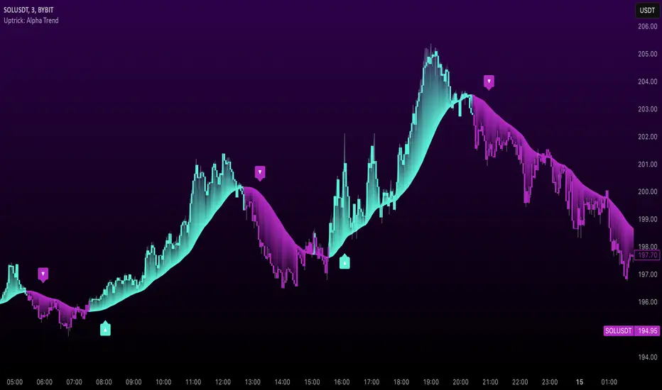
Momentum Theory Quick BiasMomentum Theory Quick Bias is a watchlist screener tool for rapid multi-timeframe analysis. It displays a variety of information from higher timeframes in order to set a directional bias including: breakout levels, peak levels, previous bar closes, and swing points.
✅ 8 Symbol Watchlist Scanner
✅ Quickly Set Directional Bias
✅ For Scalpers, Day Traders, and Swing Traders
--- 📷 INDICATOR GALLERY ---
--- 🚀 QUICK LOOK ---
✔ Multi-Timeframe Analysis
Displays various higher timeframe information in order to read how an asset is moving with one quick glance. Utilizes icons and colors that serve as visual cues.
--- ⚡ FEATURES ---
✔ Breakout Bias
Shows if the current price is above or below the breakout level on the timeframe.
✔ Peak Bias
Shows if the current previous peak has been triggered and where price is relative to it.
✔ Previous Bar Close
Shows how the previous bar closed and whether it's bullish or bearish.
Breakout
Fakeout
Inside
Outside
✔ Swing Point
Shows if the timeframe has currently flipped its breakout level.
✔ Bias Alignment
Shows visual icons if there is bias alignment between the timeframes.
↗️↘️ Breakout Bias Alignment
🔼🔽 Peak Bias Alignment
🔀 Breakout and Peak Bias Alignment, but opposite
✅ Breakout and Peak Bias Alignment
✔ Quick Analysis
Hover over the symbol name to view which timeframe levels are bullish or bearish and if peak levels have been triggered.
--- 🔥 OTHER FEATURES ---
✔ Built-In Presets
Create your own custom watchlist or use one of the built-in ones (using Oanda charts)
It's recommended to use the same source for all assets in your watchlist whenever possible
✔ Customized Layouts
Display the watchlist in a variety of different column arrangements.
✔ Dark and Light Modes
Adjustable theme colors to trade your chart the way you want.
✔ Plug-and-Play
Automatically changes the relevant levels depending on the viewed timeframe. Just fill in your watchlist, add it to your chart, and start trading!
Set the indicator to the following timeframes to view those arrangements:
Month Timeframe - Y / 6M / 3M / M
Week Timeframe - 6M / 3M / M / W
Day Timeframe - 3M / M / W / D
H4 Timeframe - Y / M / W / D
M15 Timeframe - M / W / D / H8
M10 Timeframe - M / W / D / H4
M5 Timeframe - W / D / H8 / H2
M3 Timeframe - W / D / H4 / H1
M2 Timeframe - D / H8 / H2 / M30
M1 Timeframe - D / H4 / H1 / M15
--- 📝 HOW TO USE ---
1) Create your watchlist or use one of the built-in presets and place it on the timeframe you want to see. If no watchlist is created, it automatically sets to the current asset.
2) Alignments will trigger in real-time and push to the top of the column.
It is recommended to place the indicator in a different chart window, so it won't have to refresh every time the asset or timeframe changes.
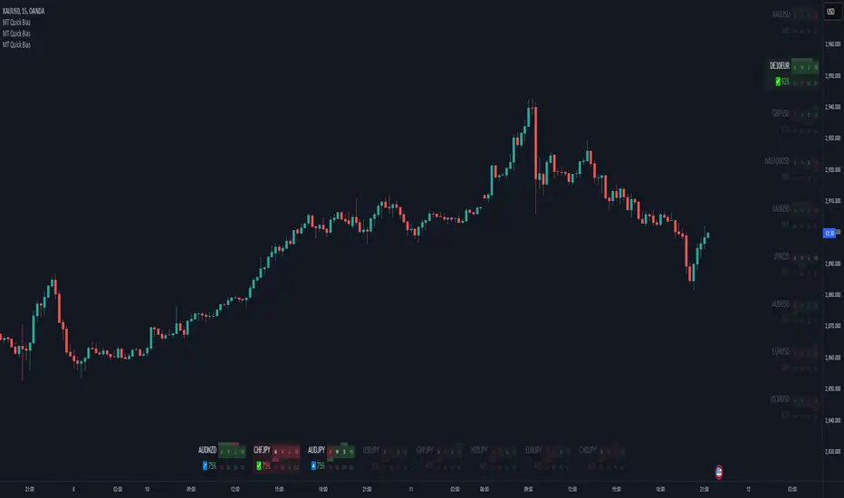
Pearson Correlation CoefficientDescription: The Pearson Correlation Coefficient measures the strength and direction of the linear relationship between two data series. Its value ranges from -1 to +1, where:
+1 indicates a perfect positive linear correlation: as one asset increases, the other asset increases proportionally.
0 indicates no linear correlation: variations in one asset have no relation to variations in the other asset.
-1 indicates a perfect negative linear correlation: as one asset increases, the other asset decreases proportionally.
This measure is widely used in technical analysis to assess the degree of correlation between two financial assets. The "Pearson Correlation (Manual Compare)" indicator allows users to manually select two assets and visually display their correlation relationship on a chart.
Features:
Correlation Period: The time period used for calculating the correlation can be adjusted (default: 50).
Comparison Asset: Users can select a secondary asset for comparison.
Visual Plots: The chart includes reference lines for perfect correlations (+1 and -1) and strong correlations (+0.7 and -0.7).
Alerts: Set alerts for when the correlation exceeds certain threshold values (e.g., +0.7 for strong positive correlation).
How to Select the Second Asset:
Primary Asset Selection: The primary asset is the one you select for viewing on the chart. This can be done by simply opening the chart for the desired asset.
Secondary Asset Selection: To select the secondary asset for comparison, use the input field labeled "Comparison Asset" in the script settings. You can manually enter the ticker symbol of the secondary asset you want to compare with the primary asset.
This indicator is ideal for traders looking to identify relationships and correlations between different financial assets to make informed trading decisions.
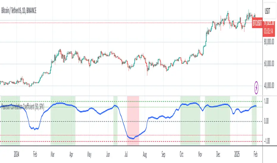
ELHAI Futures Trend Checker (ES, NQ, YM)The ELHAI Futures Trend Checker is a powerful TradingView indicator designed for futures traders who want to monitor the trend synchronization of the three major U.S. futures indices:
✅ E-mini S&P 500 (ES1!)
✅ E-mini Nasdaq 100 (NQ1!)
✅ E-mini Dow Jones (YM1!)
This indicator checks whether all three futures indices are bullish or bearish during each candle formation. If one of them is out of sync (e.g., two indices are bullish while one is bearish), the indicator triggers an alert and highlights the background in red, helping traders identify potential market indecision or divergence.
Key Features
📌 Designed for Futures Traders – Focuses on ES, NQ, and YM futures contracts.
📌 Live Market Monitoring – Works in real-time and updates dynamically with each tick.
📌 Bullish/Bearish Trend Confirmation – Detects when all three indices are in sync.
📌 Mismatch Detection – Alerts you when at least one index is out of trend.
📌 Custom Alerts – Set up TradingView alerts to be notified instantly when a trend mismatch occurs.
📌 Visual Background Highlight – A red background warns of a market divergence.
How It Works
The script retrieves open and close prices for ES, NQ, and YM.
Determines whether each futures index is bullish (close > open) or bearish (close < open).
If all three indices are bullish or all are bearish, it remains neutral.
If one index is different, an alert is triggered and the background turns red.
How to Use
Apply the indicator to your TradingView chart.
Choose any timeframe – Works well on intraday, daily, or higher timeframes.
Enable alerts: Go to Alerts → Create Alert, select "Futures Trend Mismatch", and set your preferred alert frequency.
Use alongside other indicators like moving averages, RSI, or MACD for better trade confirmation.
Best Use Cases
✔ Day traders & scalpers – Quickly spot market divergence in live trading.
✔ Swing traders – Identify when futures markets lose synchronization.
✔ Trend followers – Confirm if all major futures markets are aligned before making a move.
Final Notes
This indicator was built for Elhai to provide real-time trend analysis across major U.S. futures indices. Use it as a confirmation tool to improve market timing and decision-making.
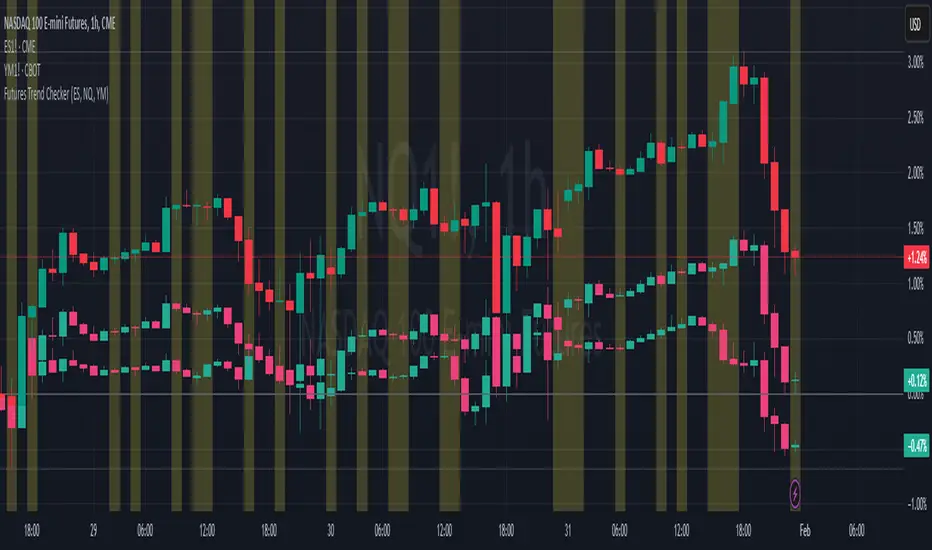
Custom Support LineIt is made with the following conditions in mind.
1. At the center of the candle at the moment,
Out of the last 10 candles, the low price (L) is within 3% of each other, drawing one line at the low prices of the candles.
2. Out of the last 10 candles, the market price (O) is within 3% of each other, drawing one line at the low end of each candle.
3.Out of the last 10 candles, the closing price (C) is within 3% of each other, and one line is drawn at the lower prices of the candles.
4. Draw one line when the three lines match the above three conditions.
We wanted to create a clear support line according to the above conditions.
