Enhanced Forex IndicatorDescription of the "Enhanced Forex Indicator"
The "Enhanced Forex Indicator" is designed for traders who want a comprehensive technical analysis tool on the TradingView platform. This script integrates Exponential Moving Averages (EMAs), support and resistance zones, and candlestick pattern recognition to provide actionable trading signals, particularly useful for Forex and other financial markets. The script is suitable for intraday trading and swing trading.
Components of the Indicator
Exponential Moving Averages (EMAs):
Short EMA (Blue Line): Faster responding average, good for identifying recent trend changes.
Long EMA (Red Line): Slower moving average, helps in confirming longer-term trends.
Support and Resistance Zones:
Resistance Zone (Red): Area where potential selling pressure could overcome buying pressure, halting price increases temporarily or reversing them.
Support Zone (Green): Area where potential buying pressure could overcome selling pressure, supporting prices and preventing them from falling further.
Candlestick Patterns:
Bullish Engulfing Pattern (Green Triangle Up 'BE'): Suggests a potential upward reversal or start of a bullish trend.
Bearish Engulfing Pattern (Red Triangle Down 'BE'): Indicates a potential downward reversal or start of a bearish trend.
Buy/Sell Signals:
Buy Signal (Green Label 'BUY'): Triggered when the price is above both EMAs and a bullish engulfing pattern is detected.
Sell Signal (Red Label 'SELL'): Triggered when the price is below both EMAs and a bearish engulfing pattern is detected.
Trading Setup:
Entry: Consider entering a buy position when the 'BUY' signal appears, indicating bullish conditions. Enter a sell position when the 'SELL' signal appears, indicating bearish conditions.
Exit: Look for closing signals opposite your entry or use predefined take profit and stop loss levels. For instance, exit a buy position on a 'SELL' signal or when the price drops below the support zone.
Risk Management:
Set stop losses just below the support zone for buy orders and above the resistance zone for sell orders to protect against significant losses.
Adjust position sizes according to your risk tolerance and account balance.
Considerations:
Use this indicator in conjunction with other analysis tools and fundamental data to confirm signals and strengthen your trading strategy.
Periodically backtest the strategy based on this indicator to ensure its effectiveness in current market conditions.
Optimization:
Adjust the lengths of the EMAs and the buffer size of the support and resistance zones to better fit the asset's volatility and your trading timeframe.
Search in scripts for "pattern"

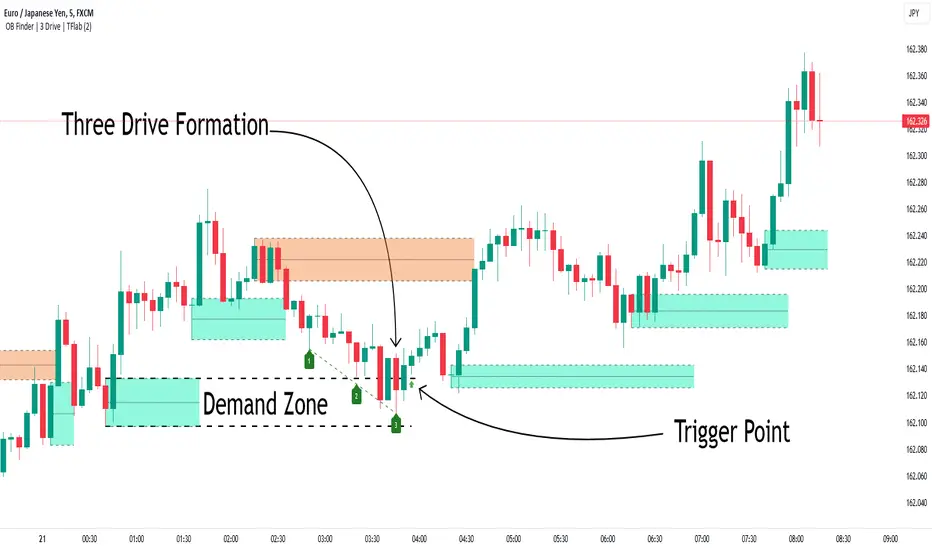
Smart Money Setup 04 [TradingFinder] Three Drive (Harmonic) + OB🔵 Introduction
The "Three Drive" pattern is a well-known formation in technical analysis, recognized for its ability to signal potential trend reversals in price action. Within the realm of trading, particularly in the context of "Reversal Patterns," the Three Drive pattern holds significance as a reliable indicator of shifts in market sentiment.
🟣 Bullish 3 Drive
This pattern typically manifests at a price bottom, where a sequence of lower lows suggests a prevailing negative trend. However, within the structure of the Three Drive pattern, a notable occurrence unfolds.
The second low breaches the range of the first low, followed by the third low surpassing the range of the second low. These penetrations signify a diminishing selling pressure and an emerging buying interest.
Traders often await the confirmation of the third low surpassing the second low as an entry point, with price targets set at the highs formed within the Three Drive pattern.
🟣 Bearish 3 Drive
Conversely, the Bearish Three Drive pattern emerges at a price top, characterized by a sequence of higher highs indicating an upward trend. Yet, amidst this apparent bullish momentum, a shift occurs.
The second high breaks beyond the range of the first high, succeeded by the third high exceeding the range of the second high. These breaches signify a waning buying strength and a resurgence in selling pressure.
Entry into a trade is often executed after the confirmation of the third high surpassing the second high, with targets set at the lows formed within the Three Drive pattern.
Importance :
Understanding the Three Drive pattern's significance extends beyond mere technical analysis. It bears resemblance to other established patterns, such as the Harmonic Pattern and Ending Diagonal within the Elliott Wave Theory.
Recognizing these parallels aids traders in comprehending broader market dynamics and potential price movements.
🔵 Formation of 3 Drive in Order Block Zone
The convergence of the Three Drive pattern with the concept of the Order Block Zone introduces a nuanced layer to traders' analytical approach.
In "Price Action" methodology, Order Blocks represent areas on the price chart where significant market players, such as institutional traders, have executed notable orders.
These zones often act as barriers, with price encountering resistance or support upon reaching them.
When the Three Drive pattern forms within an Order Block Zone, it signifies a confluence of market dynamics.
The completion of the pattern within this zone suggests a potential reversal in the prevailing trend, augmented by the presence of significant institutional orders.
Traders incorporate these Order Blocks into their analysis to identify probable levels where price may change direction, enhancing the reliability of their trading decisions.
🔵 How to Use :
To effectively utilize the Three Drive pattern within the Order Block Zone, traders seek alignment between the completion of the pattern and the presence of significant Order Blocks.
This convergence enhances the reliability of the pattern's signals, increasing the likelihood of successful trade outcomes.
Bullish Three Drive in Demand Zone :
Bearish Three Drive in Supply Zone :
Settings :
You can set your desired "Pivot Period" via settings for the indicator to identify setups based on it.
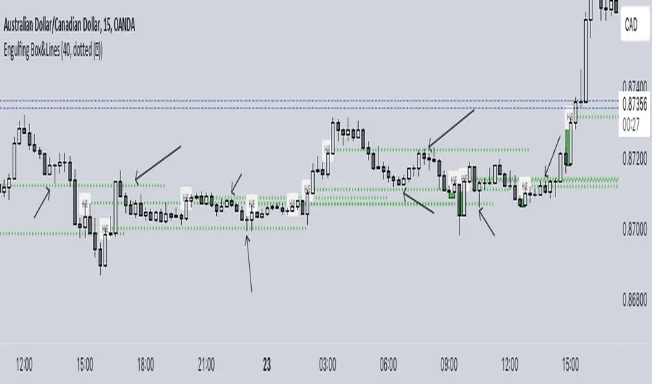
Engulfing Box & LinesThe "Engulfing Box & Lines" indicator aims to spot and highlight Engulfing candlestick patterns within a trend. These patterns can provide valuable indications of a possible trend reversal, and the indicator underlines them through the use of colored rectangles and horizontal lines. To fully understand the functioning and use of this indicator, let's explore its key elements and associated strategies.
Identification of Engulfing Patterns:
The indicator focuses on detecting two types of Engulfing candles:
Bullish Engulfing: Occurs when a bullish candle (open lower than close) completely encloses the body of the previous bearish candle. This could indicate a possible upside reversal.
Bearish Engulfing: Occurs when a bearish candle (opening higher than closing) entirely engulfs the body of the previous bullish candle. This could signal a potential bearish reversal.
Using the EMA 200:
The indicator uses the 200-period Exponential Moving Average (EMA) as a reference to determine the position of the candles with respect to the long-term trend. When the price is above the 200 EMA, the bullish Engulfing candles are highlighted with a green box, while below the 200 EMA, red boxes are shown for the bearish Engulfing candles.
Size of Boxes and Lines:
The colored boxes represent the size of the body of the candle that caused the Engulfing. Additionally, a horizontal line is drawn close to the body of the candle, serving as the fulcrum of the indicator.
Trading Strategies:
This indicator can be used for different trading strategies:
Trend Continuation: During a positive trend, the onset of an engulfing pattern suggests a possible continuation of the trend. The horizontal lines represent potential support areas, where the price could bounce. Traders might consider buying during such bounces.
Retracements and Entries: Lines can act as support or resistance zones, depending on the trend. When the price approaches a line, a retracement could occur. Traders might move to a lower timeframe to spot entry signals, using the line as a reference.
Closing Positions: Lines could also be used to define exit levels. For example, a trader might decide to exit a position when the price approaches a resistance line.
Confirmations with Other Indicators: The indicator could be used in conjunction with other technical tools, such as oscillators or candlestick analysis, to confirm signals and improve the accuracy of trading decisions.
RSI Primed [ChartPrime]
RSI Primed combines candlesticks, patterns, and the classic RSI indicator for advanced market trend indications
Introduction
Technical traders are always looking for innovative methods to pinpoint potential entry and exit points in the market. The RSI Prime indicator provides such traders with an enhanced view of market conditions by combining various charting styles and the Relative Strength Index (RSI). It offers users a unique perspective on the market trends and price momentum, enabling them to make better-informed decisions and stay ahead of the market curve.
The RSI Primed is a versatile indicator that combines different charting styles with the Relative Strength Index (RSI) to help traders analyze market trends and price momentum. It offers multiple visualization modes that serve specific purposes and provide unique insights into market performance:
Regular Candlesticks
Candlesticks with Patterns
Heikin Ashi Candles
Line Style
Regular Candlestick Mode
The Regular Candlestick Mode in RSI Primed depicts traditional Japanese candlesticks that most traders are familiar with. This mode bypasses any smoothing or modified calculations, representing real-price movements. Regular candlesticks offer a clear and straightforward way to visualize market trends and price action.
Candlestick with Patterns Mode
The Candlestick with Patterns Mode focuses on identifying high-probability candlestick patterns while incorporating RSI values. By leveraging the information captured by the RSI, this mode allows traders to spot significant market reversals or continuation patterns that could signal potential trading opportunities. Some recognizable patterns include engulfing bullish, engulfing bearish, morning star bullish, and evening star bearish patterns.
Heikin Ashi Candles Mode
The Heikin Ashi Candles Mode presents an advanced candlestick charting technique known for its excellent trend-following capabilities. Heikin Ashi Candles filter out noise in the market and provide a clear representation of market trends. In this mode, candlesticks are plotted based on RSI values of the open, high, low, and close prices, helping traders understand and utilize market trends effectively.
Line Style Mode
The Line Style Mode offers a simpler and minimalistic representation of the RSI values by using a line instead of candlesticks to visualize market trends. This mode helps traders focus on the overall trend direction and eliminates potential distractions caused by the complexity of candlestick patterns.
Candle Color Overlay Mode
The Candle Color Overlay Mode is a unique feature in the RSI Primed indicator that allows traders to visualize the RSI values on the chart's candles as a heat gradient. This mode adds a color overlay to the candlesticks, representing the RSI values in relation to the candlesticks' price action.
By displaying the RSI as a color gradient, traders can quickly assess market momentum and identify overbought or oversold conditions without having to switch between different modes or charts. The gradient ranges from cool colors (blue and green) for lower RSI values, indicating oversold conditions, to warm colors (orange and red) for higher RSI values, signifying overbought situations.
To enable the Candle Color Overlay Mode, traders can toggle the "Color Candles" option in the indicator settings. Once enabled, the color gradient will be applied to the candlesticks on the chart, providing a visually striking and informative representation of the RSI values in relation to price action. This mode can be used in tandem with any of the other charting styles, allowing traders to gain even more insights into market trends and momentum.
RSI Primed Implementation
The RSI Primed indicator combines the benefits of various charting styles with the RSI to help traders gain a comprehensive view of market trends and price momentum. It incorporates the Heikin Ashi and RSI values as inputs to generate several visualization modes, enabling traders to select the one that best suits their needs.
Chebyshev Digital Audio Filter in RSI Primed Indicator
A unique feature of the RSI Primed Indicator is the incorporation of the Chebyshev Digital Audio Filter, a powerful tool that significantly influences the indicator's accuracy and responsiveness. This signal processing method brings several benefits to the context of the RSI indicator, improving its performance and capabilities.
1. Improved Signal Filtering
The Chebyshev filter excels in its ability to remove high-frequency noise and unwanted signals from the RSI data. While other filtering techniques might introduce unwanted side effects or distort the RSI data, the Chebyshev filter accurately retains the main signal components, enhancing the RSI Primed's overall accuracy and reliability.
2. Faster Response Time
The Chebyshev filter offers a faster response time than most other filtering techniques. In the context of the RSI Primed Indicator, this means that the filtering process is quicker and more efficient, allowing traders to act swiftly during rapidly changing market conditions.
3. Enhanced Trend Detection
By effectively removing noise from the RSI data, the Chebyshev filter contributes to the enhanced detection of underlying market trends. This feature helps traders identify potential entry and exit points more accurately, improving their overall trading strategy and performance.
How to Use RSI Primed
Traders can choose from different visualization modes to suit their preferences while using the RSI Primed indicator. By closely monitoring the chosen visualization mode and the position of the moving average, traders can make informed decisions about market trends.
Green candlesticks or an upward line slope indicate a bullish trend, and red candlesticks or a downward line slope suggest a bearish trend. If the candles or line are above the moving average, it could signify an uptrend, whereas a position below the moving average may indicate a downtrend.
The RSI Primed indicator offers a unique and comprehensive perspective on market trends and price momentum by combining various charting styles with the RSI. Traders can choose from different visualization modes and make well-informed decisions to capitalize on market opportunities. This innovative indicator provides a clear and concise view of the market, enabling traders to make swift decisions and enhance their trading results.

Quinn-Fernandes Fourier Transform of Filtered Price [Loxx]Down the Rabbit Hole We Go: A Deep Dive into the Mysteries of Quinn-Fernandes Fast Fourier Transform and Hodrick-Prescott Filtering
In the ever-evolving landscape of financial markets, the ability to accurately identify and exploit underlying market patterns is of paramount importance. As market participants continuously search for innovative tools to gain an edge in their trading and investment strategies, advanced mathematical techniques, such as the Quinn-Fernandes Fourier Transform and the Hodrick-Prescott Filter, have emerged as powerful analytical tools. This comprehensive analysis aims to delve into the rich history and theoretical foundations of these techniques, exploring their applications in financial time series analysis, particularly in the context of a sophisticated trading indicator. Furthermore, we will critically assess the limitations and challenges associated with these transformative tools, while offering practical insights and recommendations for overcoming these hurdles to maximize their potential in the financial domain.
Our investigation will begin with a comprehensive examination of the origins and development of both the Quinn-Fernandes Fourier Transform and the Hodrick-Prescott Filter. We will trace their roots from classical Fourier analysis and time series smoothing to their modern-day adaptive iterations. We will elucidate the key concepts and mathematical underpinnings of these techniques and demonstrate how they are synergistically used in the context of the trading indicator under study.
As we progress, we will carefully consider the potential drawbacks and challenges associated with using the Quinn-Fernandes Fourier Transform and the Hodrick-Prescott Filter as integral components of a trading indicator. By providing a critical evaluation of their computational complexity, sensitivity to input parameters, assumptions about data stationarity, performance in noisy environments, and their nature as lagging indicators, we aim to offer a balanced and comprehensive understanding of these powerful analytical tools.
In conclusion, this in-depth analysis of the Quinn-Fernandes Fourier Transform and the Hodrick-Prescott Filter aims to provide a solid foundation for financial market participants seeking to harness the potential of these advanced techniques in their trading and investment strategies. By shedding light on their history, applications, and limitations, we hope to equip traders and investors with the knowledge and insights necessary to make informed decisions and, ultimately, achieve greater success in the highly competitive world of finance.
█ Fourier Transform and Hodrick-Prescott Filter in Financial Time Series Analysis
Financial time series analysis plays a crucial role in making informed decisions about investments and trading strategies. Among the various methods used in this domain, the Fourier Transform and the Hodrick-Prescott (HP) Filter have emerged as powerful techniques for processing and analyzing financial data. This section aims to provide a comprehensive understanding of these two methodologies, their significance in financial time series analysis, and their combined application to enhance trading strategies.
█ The Quinn-Fernandes Fourier Transform: History, Applications, and Use in Financial Time Series Analysis
The Quinn-Fernandes Fourier Transform is an advanced spectral estimation technique developed by John J. Quinn and Mauricio A. Fernandes in the early 1990s. It builds upon the classical Fourier Transform by introducing an adaptive approach that improves the identification of dominant frequencies in noisy signals. This section will explore the history of the Quinn-Fernandes Fourier Transform, its applications in various domains, and its specific use in financial time series analysis.
History of the Quinn-Fernandes Fourier Transform
The Quinn-Fernandes Fourier Transform was introduced in a 1993 paper titled "The Application of Adaptive Estimation to the Interpolation of Missing Values in Noisy Signals." In this paper, Quinn and Fernandes developed an adaptive spectral estimation algorithm to address the limitations of the classical Fourier Transform when analyzing noisy signals.
The classical Fourier Transform is a powerful mathematical tool that decomposes a function or a time series into a sum of sinusoids, making it easier to identify underlying patterns and trends. However, its performance can be negatively impacted by noise and missing data points, leading to inaccurate frequency identification.
Quinn and Fernandes sought to address these issues by developing an adaptive algorithm that could more accurately identify the dominant frequencies in a noisy signal, even when data points were missing. This adaptive algorithm, now known as the Quinn-Fernandes Fourier Transform, employs an iterative approach to refine the frequency estimates, ultimately resulting in improved spectral estimation.
Applications of the Quinn-Fernandes Fourier Transform
The Quinn-Fernandes Fourier Transform has found applications in various fields, including signal processing, telecommunications, geophysics, and biomedical engineering. Its ability to accurately identify dominant frequencies in noisy signals makes it a valuable tool for analyzing and interpreting data in these domains.
For example, in telecommunications, the Quinn-Fernandes Fourier Transform can be used to analyze the performance of communication systems and identify interference patterns. In geophysics, it can help detect and analyze seismic signals and vibrations, leading to improved understanding of geological processes. In biomedical engineering, the technique can be employed to analyze physiological signals, such as electrocardiograms, leading to more accurate diagnoses and better patient care.
Use of the Quinn-Fernandes Fourier Transform in Financial Time Series Analysis
In financial time series analysis, the Quinn-Fernandes Fourier Transform can be a powerful tool for isolating the dominant cycles and frequencies in asset price data. By more accurately identifying these critical cycles, traders can better understand the underlying dynamics of financial markets and develop more effective trading strategies.
The Quinn-Fernandes Fourier Transform is used in conjunction with the Hodrick-Prescott Filter, a technique that separates the underlying trend from the cyclical component in a time series. By first applying the Hodrick-Prescott Filter to the financial data, short-term fluctuations and noise are removed, resulting in a smoothed representation of the underlying trend. This smoothed data is then subjected to the Quinn-Fernandes Fourier Transform, allowing for more accurate identification of the dominant cycles and frequencies in the asset price data.
By employing the Quinn-Fernandes Fourier Transform in this manner, traders can gain a deeper understanding of the underlying dynamics of financial time series and develop more effective trading strategies. The enhanced knowledge of market cycles and frequencies can lead to improved risk management and ultimately, better investment performance.
The Quinn-Fernandes Fourier Transform is an advanced spectral estimation technique that has proven valuable in various domains, including financial time series analysis. Its adaptive approach to frequency identification addresses the limitations of the classical Fourier Transform when analyzing noisy signals, leading to more accurate and reliable analysis. By employing the Quinn-Fernandes Fourier Transform in financial time series analysis, traders can gain a deeper understanding of the underlying financial instrument.
Drawbacks to the Quinn-Fernandes algorithm
While the Quinn-Fernandes Fourier Transform is an effective tool for identifying dominant cycles and frequencies in financial time series, it is not without its drawbacks. Some of the limitations and challenges associated with this indicator include:
1. Computational complexity: The adaptive nature of the Quinn-Fernandes Fourier Transform requires iterative calculations, which can lead to increased computational complexity. This can be particularly challenging when analyzing large datasets or when the indicator is used in real-time trading environments.
2. Sensitivity to input parameters: The performance of the Quinn-Fernandes Fourier Transform is dependent on the choice of input parameters, such as the number of harmonic periods, frequency tolerance, and Hodrick-Prescott filter settings. Choosing inappropriate parameter values can lead to inaccurate frequency identification or reduced performance. Finding the optimal parameter settings can be challenging, and may require trial and error or a more sophisticated optimization process.
3. Assumption of stationary data: The Quinn-Fernandes Fourier Transform assumes that the underlying data is stationary, meaning that its statistical properties do not change over time. However, financial time series data is often non-stationary, with changing trends and volatility. This can limit the effectiveness of the indicator and may require additional preprocessing steps, such as detrending or differencing, to ensure the data meets the assumptions of the algorithm.
4. Limitations in noisy environments: Although the Quinn-Fernandes Fourier Transform is designed to handle noisy signals, its performance may still be negatively impacted by significant noise levels. In such cases, the identification of dominant frequencies may become less reliable, leading to suboptimal trading signals or strategies.
5. Lagging indicator: As with many technical analysis tools, the Quinn-Fernandes Fourier Transform is a lagging indicator, meaning that it is based on past data. While it can provide valuable insights into historical market dynamics, its ability to predict future price movements may be limited. This can result in false signals or late entries and exits, potentially reducing the effectiveness of trading strategies based on this indicator.
Despite these drawbacks, the Quinn-Fernandes Fourier Transform remains a valuable tool for financial time series analysis when used appropriately. By being aware of its limitations and adjusting input parameters or preprocessing steps as needed, traders can still benefit from its ability to identify dominant cycles and frequencies in financial data, and use this information to inform their trading strategies.
█ Deep-dive into the Hodrick-Prescott Fitler
The Hodrick-Prescott (HP) filter is a statistical tool used in economics and finance to separate a time series into two components: a trend component and a cyclical component. It is a powerful tool for identifying long-term trends in economic and financial data and is widely used by economists, central banks, and financial institutions around the world.
The HP filter was first introduced in the 1990s by economists Robert Hodrick and Edward Prescott. It is a simple, two-parameter filter that separates a time series into a trend component and a cyclical component. The trend component represents the long-term behavior of the data, while the cyclical component captures the shorter-term fluctuations around the trend.
The HP filter works by minimizing the following objective function:
Minimize: (Sum of Squared Deviations) + λ (Sum of Squared Second Differences)
Where:
1. The first term represents the deviation of the data from the trend.
2. The second term represents the smoothness of the trend.
3. λ is a smoothing parameter that determines the degree of smoothness of the trend.
The smoothing parameter λ is typically set to a value between 100 and 1600, depending on the frequency of the data. Higher values of λ lead to a smoother trend, while lower values lead to a more volatile trend.
The HP filter has several advantages over other smoothing techniques. It is a non-parametric method, meaning that it does not make any assumptions about the underlying distribution of the data. It also allows for easy comparison of trends across different time series and can be used with data of any frequency.
Another significant advantage of the HP Filter is its ability to adapt to changes in the underlying trend. This feature makes it particularly well-suited for analyzing financial time series, which often exhibit non-stationary behavior. By employing the HP Filter to smooth financial data, traders can more accurately identify and analyze the long-term trends that drive asset prices, ultimately leading to better-informed investment decisions.
However, the HP filter also has some limitations. It assumes that the trend is a smooth function, which may not be the case in some situations. It can also be sensitive to changes in the smoothing parameter λ, which may result in different trends for the same data. Additionally, the filter may produce unrealistic trends for very short time series.
Despite these limitations, the HP filter remains a valuable tool for analyzing economic and financial data. It is widely used by central banks and financial institutions to monitor long-term trends in the economy, and it can be used to identify turning points in the business cycle. The filter can also be used to analyze asset prices, exchange rates, and other financial variables.
The Hodrick-Prescott filter is a powerful tool for analyzing economic and financial data. It separates a time series into a trend component and a cyclical component, allowing for easy identification of long-term trends and turning points in the business cycle. While it has some limitations, it remains a valuable tool for economists, central banks, and financial institutions around the world.
█ Combined Application of Fourier Transform and Hodrick-Prescott Filter
The integration of the Fourier Transform and the Hodrick-Prescott Filter in financial time series analysis can offer several benefits. By first applying the HP Filter to the financial data, traders can remove short-term fluctuations and noise, effectively isolating the underlying trend. This smoothed data can then be subjected to the Fourier Transform, allowing for the identification of dominant cycles and frequencies with greater precision.
By combining these two powerful techniques, traders can gain a more comprehensive understanding of the underlying dynamics of financial time series. This enhanced knowledge can lead to the development of more effective trading strategies, better risk management, and ultimately, improved investment performance.
The Fourier Transform and the Hodrick-Prescott Filter are powerful tools for financial time series analysis. Each technique offers unique benefits, with the Fourier Transform being adept at identifying dominant cycles and frequencies, and the HP Filter excelling at isolating long-term trends from short-term noise. By combining these methodologies, traders can develop a deeper understanding of the underlying dynamics of financial time series, leading to more informed investment decisions and improved trading strategies. As the financial markets continue to evolve, the combined application of these techniques will undoubtedly remain an essential aspect of modern financial analysis.
█ Features
Endpointed and Non-repainting
This is an endpointed and non-repainting indicator. These are crucial factors that contribute to its usefulness and reliability in trading and investment strategies. Let us break down these concepts and discuss why they matter in the context of a financial indicator.
1. Endpoint nature: An endpoint indicator uses the most recent data points to calculate its values, ensuring that the output is timely and reflective of the current market conditions. This is in contrast to non-endpoint indicators, which may use earlier data points in their calculations, potentially leading to less timely or less relevant results. By utilizing the most recent data available, the endpoint nature of this indicator ensures that it remains up-to-date and relevant, providing traders and investors with valuable and actionable insights into the market dynamics.
2. Non-repainting characteristic: A non-repainting indicator is one that does not change its values or signals after they have been generated. This means that once a signal or a value has been plotted on the chart, it will remain there, and future data will not affect it. This is crucial for traders and investors, as it offers a sense of consistency and certainty when making decisions based on the indicator's output.
Repainting indicators, on the other hand, can change their values or signals as new data comes in, effectively "repainting" the past. This can be problematic for several reasons:
a. Misleading results: Repainting indicators can create the illusion of a highly accurate or successful trading system when backtesting, as the indicator may adapt its past signals to fit the historical price data. This can lead to overly optimistic performance results that may not hold up in real-time trading.
b. Decision-making uncertainty: When an indicator repaints, it becomes challenging for traders and investors to trust its signals, as the signal that prompted a trade may change or disappear after the fact. This can create confusion and indecision, making it difficult to execute a consistent trading strategy.
The endpoint and non-repainting characteristics of this indicator contribute to its overall reliability and effectiveness as a tool for trading and investment decision-making. By providing timely and consistent information, this indicator helps traders and investors make well-informed decisions that are less likely to be influenced by misleading or shifting data.
Inputs
Source: This input determines the source of the price data to be used for the calculations. Users can select from options like closing price, opening price, high, low, etc., based on their preferences. Changing the source of the price data (e.g., from closing price to opening price) will alter the base data used for calculations, which may lead to different patterns and cycles being identified.
Calculation Bars: This input represents the number of past bars used for the calculation. A higher value will use more historical data for the analysis, while a lower value will focus on more recent price data. Increasing the number of past bars used for calculation will incorporate more historical data into the analysis. This may lead to a more comprehensive understanding of long-term trends but could also result in a slower response to recent price changes. Decreasing this value will focus more on recent data, potentially making the indicator more responsive to short-term fluctuations.
Harmonic Period: This input represents the harmonic period, which is the number of harmonics used in the Fourier Transform. A higher value will result in more harmonics being used, potentially capturing more complex cycles in the price data. Increasing the harmonic period will include more harmonics in the Fourier Transform, potentially capturing more complex cycles in the price data. However, this may also introduce more noise and make it harder to identify clear patterns. Decreasing this value will focus on simpler cycles and may make the analysis clearer, but it might miss out on more complex patterns.
Frequency Tolerance: This input represents the frequency tolerance, which determines how close the frequencies of the harmonics must be to be considered part of the same cycle. A higher value will allow for more variation between harmonics, while a lower value will require the frequencies to be more similar. Increasing the frequency tolerance will allow for more variation between harmonics, potentially capturing a broader range of cycles. However, this may also introduce noise and make it more difficult to identify clear patterns. Decreasing this value will require the frequencies to be more similar, potentially making the analysis clearer, but it might miss out on some cycles.
Number of Bars to Render: This input determines the number of bars to render on the chart. A higher value will result in more historical data being displayed, but it may also slow down the computation due to the increased amount of data being processed. Increasing the number of bars to render on the chart will display more historical data, providing a broader context for the analysis. However, this may also slow down the computation due to the increased amount of data being processed. Decreasing this value will speed up the computation, but it will provide less historical context for the analysis.
Smoothing Mode: This input allows the user to choose between two smoothing modes for the source price data: no smoothing or Hodrick-Prescott (HP) smoothing. The choice depends on the user's preference for how the price data should be processed before the Fourier Transform is applied. Choosing between no smoothing and Hodrick-Prescott (HP) smoothing will affect the preprocessing of the price data. Using HP smoothing will remove some of the short-term fluctuations from the data, potentially making the analysis clearer and more focused on longer-term trends. Not using smoothing will retain the original price fluctuations, which may provide more detail but also introduce noise into the analysis.
Hodrick-Prescott Filter Period: This input represents the Hodrick-Prescott filter period, which is used if the user chooses to apply HP smoothing to the price data. A higher value will result in a smoother curve, while a lower value will retain more of the original price fluctuations. Increasing the Hodrick-Prescott filter period will result in a smoother curve for the price data, emphasizing longer-term trends and minimizing short-term fluctuations. Decreasing this value will retain more of the original price fluctuations, potentially providing more detail but also introducing noise into the analysis.
Alets and signals
This indicator featues alerts, signals and bar coloring. You have to option to turn these on/off in the settings menu.
Maximum Bars Restriction
This indicator requires a large amount of processing power to render on the chart. To reduce overhead, the setting "Number of Bars to Render" is set to 500 bars. You can adjust this to you liking.
█ Related Indicators and Libraries
Goertzel Cycle Composite Wave
Goertzel Browser
Fourier Spectrometer of Price w/ Extrapolation Forecast
Fourier Extrapolator of 'Caterpillar' SSA of Price
Normalized, Variety, Fast Fourier Transform Explorer
Real-Fast Fourier Transform of Price Oscillator
Real-Fast Fourier Transform of Price w/ Linear Regression
Fourier Extrapolation of Variety Moving Averages
Fourier Extrapolator of Variety RSI w/ Bollinger Bands
Fourier Extrapolator of Price w/ Projection Forecast
Fourier Extrapolator of Price
STD-Stepped Fast Cosine Transform Moving Average
Variety RSI of Fast Discrete Cosine Transform
loxfft

Custom XABCD Validation and Backtesting ToolOverview:
We hear a lot about Gartleys, bats, crabs and the rest of the barnyard crew, but have you ever wondered what other creatures might be lurking out there yet to be discovered? Well wonder no longer, it's time to find out for yourself! The Custom XABCD Validation and Backtesting Tool allows you to define retracement ratios and targets for your very own patterns.
Tips:
(1) Adjust the patterns entry/stop/target configuration and see how it affects the pattern's backtesting results.
(2) Adjust the weights of pattern score components (% error, PRZ confluence, Point D/PRZ confluence), along with the entry minimum score requirements ('If score is above'), and see how it affects the patterns' results.
Pattern Scoring:
The pattern's score is an attempt to represent the quality of a pattern with a single metric. This is one of the most powerful aspects of the tool because it can quickly tell you whether a trade is worth entering. The score is based on 3 components:
(1) Retracement % Accuracy - this measures how closely a pattern's retracement ratios match your defined theoretical values. You can change the "Allowed ratio error %" in Settings to be more or less inclusive.
(2) PRZ Level Confluence - Potential Reversal Zone levels are retracements of the XA, BC, and/or XC legs. These levels indicate where a potential reversal might occur (i.e. pivot point D). The PRZ Level Confluence component measures the closeness of the two closest PRZ levels, relative to the height of the of the XA leg.
(3) Point D / PRZ Confluence - this measures the closeness of point D to either of the two closest PRZ levels (identified in the PRZ Level Confluence component above), relative to the height of the XA leg. In theory, the closer together these levels are, the higher the probability of a reversal.
While the score is percentage-based, it should not be confused with a probability. A score of 96% does not imply a 96% chance of success. It simply represents the average of the three components mentioned above, weighted according to the defined weight parameters. A score of 100% would mean that (1) all leg retracements match the defined theoretical retracement ratios exactly, (2) all PRZ retracement levels are exactly the same value, and (3) pivot point D occurred exactly at the confluent PRZ level.
Pattern scoring research has been ongoing since I introduced the concept with my Harmonic Pattern Detection, Prediction and Backtesting Tool (see below). So the way that the score is calculated is subject to change based on the results of that research.

Stock Tech Bot One ViewTechnical indicators are not limited. Hence, here is another indicator with the combination of OBV, RSI, and MACD along with support, and resistance that follows the price while honoring the moving average of 200, 90 & 50.
The default lookback period of this indicator is 21 though it is changeable as per the user's desire.
The highest high and lowest low for the last 21 days lookback period proven to be the perfect Support & Resistance as the price of particular stock values are decided by market psychology. The support and resistance lines are very important to understand the market psychology which is very well proven with price action patterns and the lines are drawn based on,
Lower Extreme = 0.1 (Changeable)
Maximum Range = 21 days highest high - 21 days lowest low.
Support Line = 21 days lowest low + (Maximum Range * Lower Extreme)
Resistance Line = 21 days highest high - (Maximum Range * Lower Extreme)
RSI - Relative strength indicator is very famous to find the market momentum within the range of 0 - 100. Though the lookback period is changeable, the 14 days lookback period is the perfect match as the momentum of market movement for the last 3 weeks will always assist to identify the market regime. Here the momentum is just to highlight the indication (green up arrow under the candle for long and red down arrow above the candle for short) of market movement though it is not very important to consider if the price of the stock respect the support & resistance lines along with volume indicator (* = violet color).
OBV - Momentum:
The on-balance volume is always going indicator on any kind of tickers, which helps to identify the buying interest. Now, applying momentum on OBV with the positive movement for at least two consecutive days gives perfect confirmation for entry. A combination of the price along with this momentum(OBV) in the chart will help us to know the whipsaw in the price.
The Symbol "*" on top of each bar shows the market interest in that particular stock. If your ticker is fundamentally strong then you can see this "*" even when the market falls.
MACD:
One of the favorites and simple indicators widely used, where the thump of the rule is not to change the length even if it is allowed. It's OK to believe blindly in certain indicator and consider it while trading. That's why the indicator changes the bar color by following the MACD histogram.
Volume:
It may be the OBV works based on the open price and close price along with volume movement, it is wise to have the volume that is plotted along with price movement that should help you to decide whether the market is greedy or fearful.
The symbol "-" on top of each bar tells you a lot and don't ignore it.
Moving Average:
Moving average is a very good trend indicator as everyone considers seeing along with the price in the chart which is not omitted while we gauge the price movement alone with volume in this indicator. The 200, 90 & 50 MA's are everyone's favorite, and the same is plotted on the chart.
As explained above, the combination of all four indicators with price movement will give us very good confidence to take entry.
Candlestick Pattern:
You should admire the techniques of the candlestick pattern as you navigate the chart from right to left. Though there are a lot of patterns that exist, it is easy to enable and disable to view the signal as the label.
Further, last but not least, the exit always depends on individual conviction and how often the individual watch the price movement, if your conviction is strong then follow the down arrow red indication. If not, then exit with a trailing stop that indicates the bar with orange color.
Happy investing
Note: It is just a combination of multiple indicators and patterns to get one holistic view. So, the credit goes to all wise developers who publically published.

Regression Channel Alternative MTF█ OVERVIEW
This indicator displays 3 timeframes of parallel channel using linear regression calculation to assist manual drawing of chart patterns.
This indicator is not true Multi Timeframe (MTF) but considered as Alternative MTF which calculate 100 bars for Primary MTF, can be refer from provided line helper.
The timeframe scenarios are defined based on Position, Swing and Intraday Trader.
█ INSPIRATIONS
These timeframe scenarios are defined based on Harmonic Trading : Volume Three written by Scott M Carney.
By applying channel on each timeframe, MW or ABCD patterns can be easily identified manually.
This can also be applied on other chart patterns.
█ CREDITS
Scott M Carney, Harmonic Trading : Volume Three (Reaction vs. Reversal)
█ TIMEFRAME EXPLAINED
Higher / Distal : The (next) longer or larger comparative timeframe after primary pattern has been identified.
Primary / Clear : Timeframe that possess the clearest pattern structure.
Lower / Proximate : The (next) shorter timeframe after primary pattern has been identified.
Lowest : Check primary timeframe as main reference.
█ EXAMPLE OF USAGE / EXPLAINATION

Head & Shoulders S/R RegularThis is my take in Head & Shoulders (regular H&S)
The script will wait until a valid point E is found, which means A, C and E are alined
Then it will find the highest point between C - E -> Head (= D),
together with the highest point between A - C -> Left Shoulder (= B)
After this, the pattern is drawn, together with a 'trigger' area (E-G - E'-G' ~ 'Right shoulder area')
ONLY in this field, when a close is higher than E'-G', the figure will turn green, if lower than E-G, it will turn red, else, it will be blue
Settings:
Date range filtering
Here you can filter the patterns by setting the date period (for E)
Pivot Points -> Leftbars - Rightbars
min/max retrace AD -> E
Set the retracement for E (retracement A -> D -> E, here between 1.4 & 1.5)
% tolerance
Tolerance of Right shoulder height against Left shoulder height
0% (= the same relative height):
85% (-> now close isn't higher than E'-G' -> blue coloured):
min/max %
Sets the desired B height against D (here B is between 35-45% of D):
width R shoulder = L shoulder + x%
Sets the width of Right shoulder against Left shoulder
0% (nothing extra, just the same width as Left shoulder)
100% (Right shoulder area is double as large as the Left shoulder):
-70% (Right shoulder area much narrower than Left shoulder):
maximum visible patterns:
Set the maximum visible amount of patterns
This script uses one of the latest fantastic Pinescript features:
linefill and for ... in loop
Cheers!

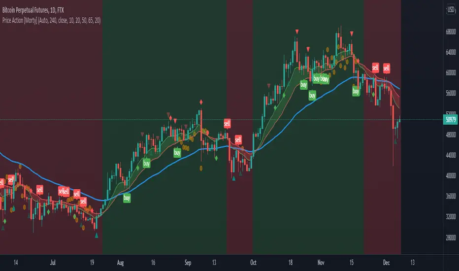
Price Action [Morty]This price action indicator uses the higher timeframe SSL channel to identify trends.
The long entry signal is a bullish candlestick pattern when the price retraces to EMA20 in an uptrend.
The short entry signal is a bearish candlestick pattern when the price retraces to the EMA20 in a downrend.
Currently, this indicator shows engulfing patterns, pin bar patterns, 2 bar reversal patterns and harami patterns.
It also shows a volatility squeeze signal when the Bollinger bands is within the Kelter channels.
The buy and sell signal can also be filter by the ADX indicator greater than a threshold.
You can set your stoploss to the previous low/high when you go long/short.
The risk/reward ratio could be 1 to 1.5.
This indicator can be used in any market.
Tweezers and Kangaroo TailHello Traders,
Here Tweezers and Kangaroo Tail script is in your service. The script searches for Tweezer / Kangaroo Tail candlestick patterns and shows them as T (Tweezer) and K (Kangaroo Tail). Thanks to RorschachT who game me the idea and some details while working on this script.
What are these candlestick patterns?
Tweezers :
- A tweezers pattern occurs when the highs/Lows of two candlesticks occur at almost exactly the same level
- Both candles must have wicks
- Bigger Wick / Smaller Wick rate should not be greater than 150% ( 150% by default and you have option to change it)
- First Candle must be highest/lowest for last 5 candles (5 by default and you have option to change it)
- The level of High for Top, Low for Bottom must be almost lower than 20% of the bigger wick of tweezer candles (20% by default and you have option to change it)
- The Candles can be right next to each other or apart but not more than 12 candles apart (12 by default and you have option to change it)
- You will see that Tweezers pattern occurs frequently
Kangaroo Tail:
- Looks almost like a Hammer or Inverted Hammer candle
- They have both its open and close in the top or bottom third of the candle
- There must be some space/room on the left of the kangaroo tail
- The open and close of the Kangaroo Tail candle must be inside the range of the previous candlestick
- The next candle should create a new high or new low
- You have several options to set details about the "Room" that should be on the left and also options for Wick/Body rates
- You can see example below
You have option to enable/disable any of these patterns.
as far as I have tested they are strong reversal patterns but none of the indicators or patterns may not be enough alone. so you should confirm the signals using other indicators or tools
If you need more information you can find a lot of info on the net ;)
Example: Tweezers - Aparted
Example: Kangaroo Tail - Bullish
Enjoy!

[RS]ZigZag PA V1ZigZag Based on price oscilation.
added pattern recognition, also added recognition of head and shoulders and contracting/expanding triangles to previous list of patterns :p
Use Alt Timeframe: enables optional timeframes, use higher timeframes to reduce noise.
Timeframe: said Alt Timeframe.
Show Patterns: toggles Pattern Recognition on.

First presented FVG (w/stats) w/statistical hourly ranges & biasOverview
This indicator identifies the first Fair Value Gap (FVG) that forms during each hourly session and provides comprehensive statistical analysis based on 12 years of historical NASDAQ (NQ) data. It combines price action analysis with probability-based statistics to help traders make informed decisions.
⚠️ IMPORTANT - Compatibility
Market: This indicator is designed exclusively for NASDAQ futures (NQ/MNQ)
Timeframe: Statistical data is based on FVGs formed on the 5-minute timeframe
FVG Detection: Works on any timeframe, but use 5-minute for accuracy matching the statistical analysis
All hardcoded statistics are derived from 12 years of NQ historical data
What It Does
1. FVG Detection & Visualization
Automatically detects the first FVG (bullish or bearish) that forms each hour
Draws colored boxes around FVGs:
Blue boxes = Bullish FVG (gap up)
Red boxes = Bearish FVG (gap down)
FVG boxes extend to the end of the hour
Optional midpoint lines show the center of each FVG
Uses volume imbalance logic (outside prints) to refine FVG boundaries
2. Hourly Reference Lines
Vertical Delimiter: Marks the start of each hour
Hourly Open Line: Shows where the current hour opened
Expected Range Lines: Projects the anticipated high/low based on historical data
Choose between Mean (average) or Median (middle value) statistics
Upper range line (teal/green)
Lower range line (red)
All lines span exactly one hour from the moment it opens
Optional labels show price values at line ends
3. Real-Time Statistics Table
The table displays live data for the current hour only:
Hour: Current hour in 12-hour format (AM/PM)
FVG Status: Shows if a Bull FVG, Bear FVG, or no FVG has formed yet
Green background = Bullish FVG detected
Red background = Bearish FVG detected
1st 15min: Direction of the first 15 minutes (Bullish/Bearish/Neutral/Pending)
Continuation %: Historical probability that the hour continues in the first 15-minute direction
Color-coded: Green for bullish, red for bearish
Avg Range %: Expected percentage range for the current hour (based on 12-year mean)
FVG Effect %: Historical probability that FVG direction predicts hourly close direction
Shows BISI→Bull % for bullish FVGs
Shows SIBI→Bear % for bearish FVGs
Blank if no FVG has formed yet
Time Left: Countdown timer showing MM:SS remaining in the hour (updates in real-time)
Hourly Bias: Historical directional tendency (bullish % or bearish %)
H Open: Current hour's opening price
Exp Range: Projected price range (Low - High) based on historical average
Customization Options
Detection Settings:
Lower Timeframe Selection (15S, 1min, 5min) - controls FVG detection granularity
Display Settings:
FVG box colors (bullish/bearish)
Midpoint lines (show/hide, color, style)
Table Settings:
Position (9 locations: corners, edges, center)
Text size (Tiny, Small, Normal, Large)
Hourly Lines:
Toggle each line type on/off
Hour delimiter (color, width)
Open line (color, width, style)
Range lines (color, width, style)
Choose Mean or Median statistics for range calculation
Show/hide labels with customizable text size
How to Use
Apply to NQ futures chart (NQ1! or MNQ1!)
Set chart to 5-minute timeframe for optimal FVG detection matching the statistical data
Watch for the first FVG to form each hour
Reference the table for probability-based decision support:
High continuation % = strong directional bias
FVG Effect % shows reliability of the FVG signal
Time Left helps manage entries/exits within the hour
Use range lines as potential targets or reversal zones
Statistical Foundation
All statistics are derived from:
12 years of NASDAQ (NQ) historical data
Hourly analysis of FVG formation patterns
First 15-minute directional analysis
Mean and Median calculations for range expectations
Data encompasses 2,400+ samples per hour
Best Practices
✅ Use on NQ/MNQ futures only
✅ Best on 5-minute charts (matches statistical data)
✅ Combine FVG signals with continuation probabilities
✅ Use range lines as potential profit targets
✅ Watch the countdown timer for hour-end setups
❌ Do not use on other markets (statistics won't apply)
❌ Avoid using during low-liquidity hours (5PM ET has minimal data)
Technical Notes
Timezone: America/New_York (EST/EDT)
Weekend filtering: Automatically hides data during market closure
Updates in real-time on live bars
Maximum 500 boxes/lines for performance
FVG detection includes volume imbalance (body gap) refinement
Credits
Statistical analysis based on 12 years of NASDAQ historical data. FVG detection methodology follows ICT concepts with volume imbalance refinement.
Disclaimer: This indicator provides statistical analysis based on historical data. Past performance does not guarantee future results. Always use proper risk management.
Would you like me to adjust any section or add/remove anything?6-9 Session & Levels - Customizable Range Analysis Indicator
Description:
This indicator provides comprehensive session-based range analysis designed for intraday traders. It calculates and displays key levels based on a customizable session period (default 6:00-9:00 AM ET).
Core Features:
Sespastedthis is a summary for another indicator- i was hoping for something more like this in terms of content etc22:23Architected comprehensive indicator summary matching professional documentation style.The user wants me to rewrite the summary for their FVG indicator in a similar style to the example provided. The example is more structured, detailed, and professional. Let me create a comprehensive summary that follows that format:
Clear title
Description/Overview
Core Features (broken down into sections)
Input Settings Explained (detailed breakdown of all customization options)
How It Works section
Use Case
Note/Disclaimer
Let me make it thorough and match the style while being accurate to their indicator's functionality.Here's a detailed summary in that format:
Every Hour 1st FVG with Statistical Analysis - NASDAQ Hourly Trading Intelligence
Description:
This indicator identifies the first Fair Value Gap (FVG) that forms during each hourly session and provides comprehensive probability-based statistical analysis derived from 12 years of NASDAQ (NQ) historical data. It combines real-time FVG detection with hardcoded statistical probabilities to help intraday traders make informed decisions based on historical patterns and hourly price action dynamics.
IMPORTANT: This indicator is specifically calibrated for NASDAQ futures (NQ/MNQ) only. All statistical data is derived from 12 years of NQ historical analysis with FVGs detected on the 5-minute timeframe. Using this indicator on other markets will produce invalid statistical results.
Core Features:
FVG Detection & Visualization
Automatically detects and displays the first Fair Value Gap (bullish or bearish) that forms within each hourly session
Color-coded boxes mark FVG zones: Blue for bullish FVGs (gap up), Red for bearish FVGs (gap down)
FVG boxes extend precisely to the end of the hour boundary
Optional midpoint lines show the center point of each FVG
Uses volume imbalance logic (outside prints) to refine FVG boundaries beyond simple wick-to-wick gaps
Supports both chart timeframe detection and lower timeframe detection via request.security_lower_tf
Hourly Reference Lines
Vertical Hour Delimiter: Marks the exact start of each new hour with an extendable vertical line
Hourly Open Line: Displays the opening price of the current hour
Expected Range Lines: Projects anticipated high and low levels based on 12 years of statistical data
Choose between Mean (average) or Median (middle value) calculations
Upper range line shows expected high
Lower range line shows expected low
All lines span exactly one hour from open to close
Optional labels display exact price values at the end of each line
Real-Time Statistics Table
Displays comprehensive live data for the current hour only:
Hour: Current hour in 12-hour format (e.g., "9AM", "2PM")
FVG Status: Shows detection state with color coding
"None Yet" (white background) - No FVG detected
"Bull FVG" (green background) - Bullish FVG identified
"Bear FVG" (red background) - Bearish FVG identified
1st 15min: Direction of first 15 minutes (Bullish/Bearish/Neutral/Pending)
Continuation %: Historical probability that the hour closes in the direction of the first 15 minutes
Green background with up arrow (↑) for bullish continuation probability
Red background with down arrow (↓) for bearish continuation probability
Avg Range %: Expected percentage range for the current hour based on 12-year mean
FVG Effect %: Historical effectiveness of FVG directional prediction
Shows "BISI→Bull %" for bullish FVGs (gap up predicting bullish hourly close)
Shows "SIBI→Bear %" for bearish FVGs (gap down predicting bearish hourly close)
Displays blank if no FVG has formed yet
Time Left: Real-time countdown timer showing minutes and seconds remaining in the hour (MM:SS format)
Hourly Bias: Historical directional tendency showing bullish or bearish percentage bias
H Open: Current hour's opening price
Exp Range: Projected price range showing "Low - High" based on selected statistic (mean or median)
Input Settings Explained:
Detection Settings
Lower Timeframe: Select the base timeframe for FVG detection
Options: 15S (15 seconds), 1 (1 minute), 5 (5 minutes)
Recommendation: Use 5-minute to match the statistical data sample
The indicator uses this timeframe to scan for FVG patterns even when viewing higher timeframes
Display Settings
Bullish FVG Color: Set the color and transparency for bullish (upward) FVG boxes
Bearish FVG Color: Set the color and transparency for bearish (downward) FVG boxes
Show Midpoint Lines: Toggle horizontal lines at the center of each FVG box
Midpoint Line Color: Customize the midpoint line color
Midpoint Line Style: Choose between Solid, Dotted, or Dashed line styles
Table Settings
Table Position: Choose from 9 locations:
Top: Left, Center, Right
Middle: Left, Center, Right
Bottom: Left, Center, Right
Table Text Size: Select from Tiny, Small, Normal, or Large for readability on different screen sizes
Hourly Lines Settings
Show Hourly Lines: Master toggle for all hourly reference lines
Show Hour Delimiter: Toggle the vertical line marking each hour's start
Delimiter Color: Customize color and transparency
Delimiter Width: Set line thickness (1-5)
Show Hourly Open: Toggle the horizontal line at the hour's opening price
Open Line Color: Customize color
Open Line Width: Set thickness (1-5)
Open Line Style: Choose Solid, Dashed, or Dotted
Show Range Lines: Toggle the expected high/low projection lines
Range Statistic: Choose "Mean" (12-year average) or "Median" (12-year middle value)
Range High Color: Customize upper range line color and transparency
Range Low Color: Customize lower range line color and transparency
Range Line Width: Set thickness (1-5)
Range Line Style: Choose Solid, Dashed, or Dotted
Show Line Labels: Toggle price labels at the end of all horizontal lines
Label Text Size: Choose Tiny, Small, or Normal
How It Works:
FVG Detection Logic:
The indicator scans price action on the selected lower timeframe (default: 1-minute) looking for Fair Value Gaps using a 3-candle pattern:
Bullish FVG: Formed when candle 's high is below candle 's low, creating an upward gap
Bearish FVG: Formed when candle 's low is above candle 's high, creating a downward gap
The detection is refined using volume imbalance logic by checking for body gaps (outside prints) on both sides of the middle candle. This narrows the FVG zone to areas where bodies don't touch, indicating stronger imbalances.
Only the first FVG that forms during each hour is displayed. If a bullish FVG forms first, it takes priority. The FVG box is drawn from the formation time through to the end of the hour.
Statistical Analysis:
All probability statistics are hardcoded from 12 years (2,400+ samples per hour) of NASDAQ futures analysis:
First 15-Minute Direction: At 15 minutes into each hour, the indicator determines if price closed above, below, or equal to the hour's opening price
Continuation Probability: Historical analysis shows the likelihood that the hour closes in the same direction as the first 15 minutes
Example: If 9AM's first 15 minutes are bullish, there's a 60.1% chance the entire 9AM hour closes bullish (lowest continuation hour)
4PM shows the highest continuation at 86.1% for bullish first 15 minutes
FVG Effectiveness: Tracks how often the first FVG's direction correctly predicts the hourly close direction
BISI (Bullish Imbalance/Sell-side Inefficiency) → Bullish close probability
SIBI (Bearish Imbalance/Buy-side Inefficiency) → Bearish close probability
Range Expectations: Mean and median values represent typical price movement percentage for each hour
9AM and 10AM show the largest ranges (~0.6%)
5PM shows minimal range (~0.06%) due to low liquidity
Hourly Reference Lines:
When each new hour begins:
Vertical delimiter marks the hour's start
Hourly open line plots at the first bar's opening price
Range projection lines calculate expected high/low:
Upper Range = Hourly Open + (Range% / 100 × Hourly Open)
Lower Range = Hourly Open - (Range% / 100 × Hourly Open)
Lines extend exactly to the hour's end time
Labels appear at line endpoints showing exact prices
Real-Time Updates:
FVG Status: Updates immediately when the first FVG forms
First 15min Direction: Locked in at the 15-minute mark
Countdown Timer: Uses timenow to update every second
Table Statistics: Refresh on every bar close
Timezone Handling:
All times are in America/New_York (Eastern Time)
Automatically filters weekend periods (Saturday and Sunday before 6PM)
Hour detection accounts for daylight saving time changes
Use Cases:
Intraday Trading Strategy Development:
FVG Entry Signals: Use the first hourly FVG as a directional bias
Bullish FVG + High continuation % = Strong long setup
Bearish FVG + High continuation % = Strong short setup
First 15-Minute Breakout: Combine first 15-min direction with continuation probabilities
Wait for first 15 minutes to complete
If continuation % is above 70%, trade in that direction
Example: 4PM bullish first 15 min = 86.1% chance hour closes bullish
Range Targeting: Use expected high/low lines as profit targets or reversal zones
Price approaching mean high = potential resistance
Price approaching mean low = potential support
Compare mean vs median for different risk tolerance (median is more conservative)
Hour Selection: Focus trading on hours with:
High FVG effectiveness (11AM: 81.5% BISI→Bull)
High continuation rates (4PM: 86.1% bull continuation)
Avoid low-continuation hours like 9AM (60.1%)
Time Management: Use the countdown timer to:
Enter early in the hour when FVG forms
Exit before hour-end if no follow-through
Avoid late-hour entries with <15 minutes remaining
Statistical Edge Identification:
Compare current hour's FVG against historical effectiveness
Identify when first 15-min direction contradicts FVG direction (conflict = caution)
Use hourly bias to confirm or contradict FVG signals
Monitor if price stays within expected range or breaks out (outlier moves)
Risk Management:
Expected range lines provide logical stop-loss placement
FVG Effect % helps size positions (higher % = larger position)
Time Left countdown aids in time-based stop management
Avoid trading hours with neutral bias or low continuation rates
Statistical Foundation:
All embedded statistics are derived from:
12 years of NASDAQ futures (NQ) continuous contract data
5-minute timeframe FVG detection methodology
24 hours per day analysis (excluding weekends)
2,400+ samples per hour for robust statistical validity
America/New_York timezone for session alignment
Data includes:
Hourly range analysis (mean, median, standard deviation)
First 15-minute directional analysis
FVG formation frequency and effectiveness
Continuation probability matrices
Bullish/bearish bias percentages
Best Practices:
✅ Do:
Use exclusively on NASDAQ futures (NQ1! or MNQ1!)
Apply on 5-minute charts for optimal FVG detection matching statistical samples
Wait for first 15 minutes to complete before acting on continuation probabilities
Combine FVG signals with continuation % and FVG Effect % for confluence
Use expected range lines as initial profit targets
Monitor the countdown timer for time-based trade management
Focus on hours with high statistical edges (4PM, 11AM, 10AM)
❌ Don't:
Use on other markets (ES, RTY, YM, stocks, forex, crypto) - statistics will be invalid
Rely solely on FVG without confirming with continuation probabilities
Trade during low-liquidity hours (5PM shows only 0.06% average range)
Ignore the first 15-minute direction when it conflicts with FVG direction
Apply to timeframes significantly different from 5-minute for FVG detection
Use median range expectations aggressively (they're conservative)
Technical Implementation Notes:
Timezone: Fixed to America/New_York with automatic DST adjustment
Weekend Filtering: Automatically hides data Saturday and Sunday before 6PM ET
Performance: Maximum 500 boxes and 500 lines for optimal chart rendering
Update Frequency: Table updates on every bar close; timer updates every second using timenow
FVG Priority: Bullish FVGs take precedence when both form simultaneously
Lower Timeframe Detection: Uses request.security_lower_tf for accurate sub-chart-timeframe FVG detection
Precision: All price labels use format.mintick for appropriate decimal precision
Big thanks to @Trades-Dont-Lie for the FPFVG code in his excellent indicator that I've used here

Elliott Wave Full Fractal System v2.0Elliott Wave Full Fractal System v2.0 – Q.C. FINAL (Guaranteed R/R)
Elliott Wave Full Fractal System is a multi-timeframe wave engine that automatically labels Elliott impulses and ABC corrections, then builds a rule-based, ATR-driven risk/reward framework around the “W3–W4–W5” leg.
“Guaranteed R/R” here means every order is placed with a predefined stop-loss and take-profit that respect a minimum Reward:Risk ratio – it does not mean guaranteed profits.
Core Idea
This strategy turns a full fractal Elliott Wave labelling engine into a systematic trading model.
It scans fractal pivots on three wave degrees (Primary, Intermediate, Minor) to detect 5-wave impulses and ABC corrections.
A separate “Trading Degree” pivot stream, filtered by a 200-EMA trend filter and ATR-based dynamic pivots, is then used to find W4 pullback entries with a minimum, user-defined Reward:Risk ratio.
Default Properties & Risk Assumptions
The backtest uses realistic but conservative defaults:
// Default properties used for backtesting
strategy(
"Elliott Wave Full Fractal System - Q.C. FINAL (Guaranteed R/R)",
overlay = true,
initial_capital = 10000, // realistic account size
default_qty_type = strategy.percent_of_equity,
default_qty_value = 1, // 1% risk per trade
commission_type = strategy.commission.cash_per_contract,
commission_value = 0.005, // example stock commission
slippage = 0 // see notes below
)
Account size: 10,000 (can be changed to match your own account).
Position sizing: 1% of equity per trade to keep risk per idea sustainable and aligned with TradingView’s recommendations.
Commission: 0.005 cash per contract/share as a realistic example for stock trading.
Slippage: set to 0 in code for clarity of “pure logic” backtesting. Real-life trading will experience slippage, so users should adjust this according to their market and broker.
Always re-run the backtest after changing any of these values, and avoid using high risk fractions (5–10%+) as that is rarely sustainable.
1. Full Fractal Wave Engine
The script builds and maintains four pivot streams using ATR-adaptive fractals:
Primary Degree (Macro Trend):
Captures the large swings that define the major trend. Labels ①–⑤ and ⒶⒷⒸ using blue “Circle” labels and thicker lines.
Intermediate Degree (Trading Degree):
Captures the medium swings (swing-trading horizon). Uses teal labels ( (1)…(5), (A)(B)(C) ).
Minor Degree (Micro Structure):
Tracks short-term swings inside the larger waves. Uses red roman numerals (i…v, a b c).
ABC Corrections (Optional):
When enabled, the engine tries to detect standard A–B–C corrective structures that follow a completed 5-wave impulse and plots them with dashed lines.
Each degree uses a dynamic pivot lookback that expands when ATR is above its EMA, so the system naturally requires “stronger” pivots in volatile environments and reacts faster in quiet conditions.
2. Theory Rules & Strict Mode
Normal Mode: More permissive detection. Designed to show more wave structures for educational / exploratory use.
Strict Mode: Enforces key Elliott constraints:
Wave 3 not shorter than waves 1 and 5.
No invalid W4 overlap with W1 (for standard impulses).
ABC Logic: After a confirmed bullish impulse, the script expects a down-up-down corrective pattern (A,B,C). After a bearish impulse, it looks for up-down-up.
3. Trend Filter & Pivots
EMA Trend Filter: A configurable EMA (default 200) is used as a non-wave trend filter.
Price above EMA → Only long setups are considered.
Price below EMA → Only short setups are considered.
ATR-Adaptive Pivots: The pivot engine scales its left/right bars based on current ATR vs ATR EMA, making waves and trading pivots more robust in volatile regimes.
4. Dynamic Risk Management (Guaranteed R/R Engine)
The trading engine is designed around risk, not just pattern recognition:
ATR-Based Stop:
Stop-loss is placed at:
Entry ± ATR × Multiplier (user-configurable, default 2.0).
This anchors risk to current volatility.
Minimum Reward:Risk Ratio:
For each setup, the script:
Computes the distance from entry to stop (risk).
Projects a take-profit target at risk × min_rr_ratio away from entry.
Only accepts the setup if risk is positive and the required R:R ratio is achievable.
Result: Every order is created with both TP and SL at a predefined distance, so each trade starts with a known, minimum Reward:Risk profile by design.
“Guaranteed R/R” refers exclusively to this order placement logic (TP/SL geometry), not to win-rate or profitability.
5. Trading Logic – W3–W4–W5 Pattern
The Trading pivot stream (separate from visual wave degrees) looks for a simple but powerful pattern:
Bullish structure:
Sequence of pivots forms a higher-high / higher-low pattern.
Price is above the EMA trend filter.
A strong “W3” leg is confirmed with structure rules (optionally stricter in Strict mode).
Entry (Long – W4 Pullback):
The “height” of W3 is measured.
Entry is placed at a configurable Fibonacci pullback (default 50%) inside that leg.
ATR-based stop is placed below entry.
Take-profit is projected to satisfy min Reward:Risk.
Bearish structure:
Mirrored logic (lower highs/lows, price below EMA, W3 down, W4 retrace up, W5 continuation down).
Once a valid setup is found, the script draws a colored box around the entry zone and a label describing the type of signal (“LONG SETUP” or “SHORT SETUP”) with the suggested limit price.
6. Orders & Execution
Entry Orders: The strategy uses limit orders at the computed W4 level (“Sniper Long” or “Sniper Short”).
Exits: A single strategy.exit() is attached to each entry with:
Take-profit at the projected minimum R:R target.
Stop-loss at ATR-based level.
One Trade at a Time: New setups are only used when there is no open position (strategy.opentrades == 0) to keep the logic clear and risk contained.
7. Visual Guide on the Chart
Wave Labels:
Primary: ①,②,③,④,⑤, ⒶⒷⒸ
Intermediate: (1)…(5), (A)(B)(C)
Minor: i…v, a b c
Trend EMA: Single blue EMA showing the dominant trend.
Setup Boxes:
Green transparent box → long entry zone.
Red transparent box → short entry zone.
Labels: “LONG SETUP / SHORT SETUP” labels mark the proposed limit entry with price.
8. How to Use This Strategy
Attach the strategy to your chart
Choose your market (stocks, indices, FX, crypto, futures, etc.) and timeframe (for example 1h, 4h, or Daily). Then add the strategy to the chart from your Scripts list.
Start with the default settings
Leave all inputs on their defaults first. This lets you see the “intended” behaviour and the exact properties used for the published backtest (account size, 1% risk, commission, etc.).
Study the wave map
Zoom in and out and look at the three wave degrees:
Blue circles → Primary degree (big picture trend).
Teal (1)…(5) → Intermediate degree (swing structure).
Red i…v → Minor degree (micro waves).
Use this to understand how the engine is interpreting the Elliott structure on your symbol.
Watch for valid setups
Look for the coloured boxes and labels:
Green box + “LONG SETUP” label → potential W4 pullback long in an uptrend.
Red box + “SHORT SETUP” label → potential W4 pullback short in a downtrend.
Only trades in the direction of the EMA trend filter are allowed by the strategy.
Check the Reward:Risk of each idea
For each setup, inspect:
Limit entry price.
ATR-based stop level.
Projected take-profit level.
Make sure the minimum Reward:Risk ratio matches your own rules before you consider trading it.
Backtest and evaluate
Open the Strategy Tester:
Verify you have a decent sample size (ideally 100+ trades).
Check drawdowns, average trade, win-rate and R:R distribution.
Change markets and timeframes to see where the logic behaves best.
Adapt to your own risk profile
If you plan to use it live:
Set Initial Capital to your real account size.
Adjust default_qty_value to a risk level you are comfortable with (often 0.5–2% per trade).
Set commission and slippage to realistic broker values.
Re-run the backtest after every major change.
Use as a framework, not a signal machine
Treat this as a structured Elliott/R:R framework:
Filter signals by higher-timeframe trend, major S/R, volume, or fundamentals.
Optionally hide some wave degrees or ABC labels if you want a cleaner chart.
Combine the system’s structure with your own trade management and discretion.
Best Practices & Limitations
This is an approximate Elliott Wave engine based on fractal pivots. It does not replace a full discretionary Elliott analysis.
All wave counts are algorithmic and can differ from a manual analyst’s interpretation.
Like any backtest, results depend heavily on:
Symbol and timeframe.
Sample size (more trades are better).
Realistic commission/slippage settings.
The 0-slippage default is chosen only to show the “raw logic”. In real markets, slippage can significantly impact performance.
No strategy wins all the time. Losing streaks and drawdowns will still occur even with a strict R:R framework.
Disclaimer
This script is for educational and research purposes only and does not constitute financial advice or a recommendation to buy or sell any security. Past performance, whether real or simulated, is not indicative of future results. Always test on multiple symbols/timeframes, use conservative risk, and consult your financial advisor before trading live capital.

Universal Pivot ScannerUniversal Pivot Scanner
Professional pivot pattern detection for any market data source.
A robust pivot detector designed to work across all timeframes and data types - price action, technical indicators, volume, or custom studies. One tool, multiple applications.
Core Functionality
Identifies two high-probability retracement patterns:
HH+HL → Bullish continuation setup (higher high followed by higher low)
LL+LH → Bearish continuation setup (lower low followed by lower high)
Key Features
Non-repainting detection. Labels and alerts trigger at pivot confirmation, ensuring real-time actionable signals without historical bias.
Source flexibility. Compatible with any input - price data, oscillators (RSI, MACD), volume analysis, or proprietary indicators. Single implementation across multiple strategies.
Adaptive configuration. Adjustable lookback period optimizes performance for different market conditions and data types.
Recommended Settings
Lookback: 1 → Oscillators and momentum indicators
Lookback: 3-10 → Price action and ranging markets
Includes visualization table displaying recent pivot sequence and active pattern status.
Designed for systematic traders requiring consistent, verifiable signals across diverse market conditions.

CRT / ORB Signals [Yosiet]What is the CRT Pattern?
The Counter-Retracement Pattern is a classic three-candle setup that reveals moments of market structure weakness and potential reversal. It occurs when a strong move is temporarily rejected, signaling a possible continuation.
Several names for the same candlestick pattern: CRT, ORB, Morning Star, Evening Star, and others, but I'm not going to talk about it.
Here’s the anatomy of a Bullish CRT:
Candle 1 (C1: The Signal Candle): A significant momentum candle in a downtrend.
Candle 2 (C2: The Retracement/Sweep Candle): This is the critical candle. It must sweep the low of C1 (liquidity grab / sweep) but then close with its body inside the range of C1 .
Candle 3 (C3: The Confirmation/Entry Candle): A bullish candle that closes above C2's close, confirming the pattern.
Here’s the anatomy of a Bearish CRT:
The bearish pattern is the exact inverse, sweeping the high of Candle 1.
Why This Indicator?
Clarity and Precision. This script is built for accuracy and minimalism.
No Repainting: The logic is calculated on the closed historical bars. The signal is only plotted on the entry candle (Candle 3) after it has closed.
Clean Visuals: Instead of cluttering every candle, it shows you only what you need:
Green Up Arrow: Signals a confirmed Bullish CRT, suggesting a Long entry.
Red Down Arrow: Signals a confirmed Bearish CRT, suggesting a Short entry.
Faint Circles: Subtle white circles mark the high/low of Candle 1 and Candle 2, helping you visually trace the pattern structure without obstruction.

Algorithm Predator - ML-liteAlgorithm Predator - ML-lite
This indicator combines four specialized trading agents with an adaptive multi-armed bandit selection system to identify high-probability trade setups. It is designed for swing and intraday traders who want systematic signal generation based on institutional order flow patterns , momentum exhaustion , liquidity dynamics , and statistical mean reversion .
Core Architecture
Why These Components Are Combined:
The script addresses a fundamental challenge in algorithmic trading: no single detection method works consistently across all market conditions. By deploying four independent agents and using reinforcement learning algorithms to select or blend their outputs, the system adapts to changing market regimes without manual intervention.
The Four Trading Agents
1. Spoofing Detector Agent 🎭
Detects iceberg orders through persistent volume at similar price levels over 5 bars
Identifies spoofing patterns via asymmetric wick analysis (wicks exceeding 60% of bar range with volume >1.8× average)
Monitors order clustering using simplified Hawkes process intensity tracking (exponential decay model)
Signal Logic: Contrarian—fades false breakouts caused by institutional manipulation
Best Markets: Consolidations, institutional trading windows, low-liquidity hours
2. Exhaustion Detector Agent ⚡
Calculates RSI divergence between price movement and momentum indicator over 5-bar window
Detects VWAP exhaustion (price at 2σ bands with declining volume)
Uses VPIN reversals (volume-based toxic flow dissipation) to identify momentum failure
Signal Logic: Counter-trend—enters when momentum extreme shows weakness
Best Markets: Trending markets reaching climax points, over-extended moves
3. Liquidity Void Detector Agent 💧
Measures Bollinger Band squeeze (width <60% of 50-period average)
Identifies stop hunts via 20-bar high/low penetration with immediate reversal and volume spike
Detects hidden liquidity absorption (volume >2× average with range <0.3× ATR)
Signal Logic: Breakout anticipation—enters after liquidity grab but before main move
Best Markets: Range-bound pre-breakout, volatility compression zones
4. Mean Reversion Agent 📊
Calculates price z-scores relative to 50-period SMA and standard deviation (triggers at ±2σ)
Implements Ornstein-Uhlenbeck process scoring (mean-reverting stochastic model)
Uses entropy analysis to detect algorithmic trading patterns (low entropy <0.25 = high predictability)
Signal Logic: Statistical reversion—enters when price deviates significantly from statistical equilibrium
Best Markets: Range-bound, low-volatility, algorithmically-dominated instruments
Adaptive Selection: Multi-Armed Bandit System
The script implements four reinforcement learning algorithms to dynamically select or blend agents based on performance:
Thompson Sampling (Default - Recommended):
Uses Bayesian inference with beta distributions (tracks alpha/beta parameters per agent)
Balances exploration (trying underused agents) vs. exploitation (using proven winners)
Each agent's win/loss history informs its selection probability
Lite Approximation: Uses pseudo-random sampling from price/volume noise instead of true random number generation
UCB1 (Upper Confidence Bound):
Calculates confidence intervals using: average_reward + sqrt(2 × ln(total_pulls) / agent_pulls)
Deterministic algorithm favoring agents with high uncertainty (potential upside)
More conservative than Thompson Sampling
Epsilon-Greedy:
Exploits best-performing agent (1-ε)% of the time
Explores randomly ε% of the time (default 10%, configurable 1-50%)
Simple, transparent, easily tuned via epsilon parameter
Gradient Bandit:
Uses softmax probability distribution over agent preference weights
Updates weights via gradient ascent based on rewards
Best for Blend mode where all agents contribute
Selection Modes:
Switch Mode: Uses only the selected agent's signal (clean, decisive)
Blend Mode: Combines all agents using exponentially weighted confidence scores controlled by temperature parameter (smooth, diversified)
Lock Agent Feature:
Optional manual override to force one specific agent
Useful after identifying which agent dominates your specific instrument
Only applies in Switch mode
Four choices: Spoofing Detector, Exhaustion Detector, Liquidity Void, Mean Reversion
Memory System
Dual-Layer Architecture:
Short-Term Memory: Stores last 20 trade outcomes per agent (configurable 10-50)
Long-Term Memory: Stores episode averages when short-term reaches transfer threshold (configurable 5-20 bars)
Memory Boost Mechanism: Recent performance modulates agent scores by up to ±20%
Episode Transfer: When an agent accumulates sufficient results, averages are condensed into long-term storage
Persistence: Manual restoration of learned parameters via input fields (alpha, beta, weights, microstructure thresholds)
How Memory Works:
Agent generates signal → outcome tracked after 8 bars (performance horizon)
Result stored in short-term memory (win = 1.0, loss = 0.0)
Short-term average influences agent's future scores (positive feedback loop)
After threshold met (default 10 results), episode averaged into long-term storage
Long-term patterns (weighted 30%) + short-term patterns (weighted 70%) = total memory boost
Market Microstructure Analysis
These advanced metrics quantify institutional order flow dynamics:
Order Flow Toxicity (Simplified VPIN):
Measures buy/sell volume imbalance over 20 bars: |buy_vol - sell_vol| / (buy_vol + sell_vol)
Detects informed trading activity (institutional players with non-public information)
Values >0.4 indicate "toxic flow" (informed traders active)
Lite Approximation: Uses simple open/close heuristic instead of tick-by-tick trade classification
Price Impact Analysis (Simplified Kyle's Lambda):
Measures market impact efficiency: |price_change_10| / sqrt(volume_sum_10)
Low values = large orders with minimal price impact ( stealth accumulation )
High values = retail-dominated moves with high slippage
Lite Approximation: Uses simplified denominator instead of regression-based signed order flow
Market Randomness (Entropy Analysis):
Counts unique price changes over 20 bars / 20
Measures market predictability
High entropy (>0.6) = human-driven, chaotic price action
Low entropy (<0.25) = algorithmic trading dominance (predictable patterns)
Lite Approximation: Simple ratio instead of true Shannon entropy H(X) = -Σ p(x)·log₂(p(x))
Order Clustering (Simplified Hawkes Process):
Tracks self-exciting event intensity (coordinated order activity)
Decays at 0.9× per bar, spikes +1.0 when volume >1.5× average
High intensity (>0.7) indicates clustering (potential spoofing/accumulation)
Lite Approximation: Simple exponential decay instead of full λ(t) = μ + Σ α·exp(-β(t-tᵢ)) with MLE
Signal Generation Process
Multi-Stage Validation:
Stage 1: Agent Scoring
Each agent calculates internal score based on its detection criteria
Scores must exceed agent-specific threshold (adjusted by sensitivity multiplier)
Agent outputs: Signal direction (+1/-1/0) and Confidence level (0.0-1.0)
Stage 2: Memory Boost
Agent scores multiplied by memory boost factor (0.8-1.2 based on recent performance)
Successful agents get amplified, failing agents get dampened
Stage 3: Bandit Selection/Blending
If Adaptive Mode ON:
Switch: Bandit selects single best agent, uses only its signal
Blend: All agents combined using softmax-weighted confidence scores
If Adaptive Mode OFF:
Traditional consensus voting with confidence-squared weighting
Signal fires when consensus exceeds threshold (default 70%)
Stage 4: Confirmation Filter
Raw signal must repeat for consecutive bars (default 3, configurable 2-4)
Minimum confidence threshold: 0.25 (25%) enforced regardless of mode
Trend alignment check: Long signals require trend_score ≥ -2, Short signals require trend_score ≤ 2
Stage 5: Cooldown Enforcement
Minimum bars between signals (default 10, configurable 5-15)
Prevents over-trading during choppy conditions
Stage 6: Performance Tracking
After 8 bars (performance horizon), signal outcome evaluated
Win = price moved in signal direction, Loss = price moved against
Results fed back into memory and bandit statistics
Trading Modes (Presets)
Pre-configured parameter sets:
Conservative: 85% consensus, 4 confirmations, 15-bar cooldown
Expected: 60-70% win rate, 3-8 signals/week
Best for: Swing trading, capital preservation, beginners
Balanced: 70% consensus, 3 confirmations, 10-bar cooldown
Expected: 55-65% win rate, 8-15 signals/week
Best for: Day trading, most traders, general use
Aggressive: 60% consensus, 2 confirmations, 5-bar cooldown
Expected: 50-58% win rate, 15-30 signals/week
Best for: Scalping, high-frequency trading, active management
Elite: 75% consensus, 3 confirmations, 12-bar cooldown
Expected: 58-68% win rate, 5-12 signals/week
Best for: Selective trading, high-conviction setups
Adaptive: 65% consensus, 2 confirmations, 8-bar cooldown
Expected: Varies based on learning
Best for: Experienced users leveraging bandit system
How to Use
1. Initial Setup (5 Minutes):
Select Trading Mode matching your style (start with Balanced)
Enable Adaptive Learning (recommended for automatic agent selection)
Choose Thompson Sampling algorithm (best all-around performance)
Keep Microstructure Metrics enabled for liquid instruments (>100k daily volume)
2. Agent Tuning (Optional):
Adjust Agent Sensitivity multipliers (0.5-2.0):
<0.8 = Highly selective (fewer signals, higher quality)
0.9-1.2 = Balanced (recommended starting point)
1.3 = Aggressive (more signals, lower individual quality)
Monitor dashboard for 20-30 signals to identify dominant agent
If one agent consistently outperforms, consider using Lock Agent feature
3. Bandit Configuration (Advanced):
Blend Temperature (0.1-2.0):
0.3 = Sharp decisions (best agent dominates)
0.5 = Balanced (default)
1.0+ = Smooth (equal weighting, democratic)
Memory Decay (0.8-0.99):
0.90 = Fast adaptation (volatile markets)
0.95 = Balanced (most instruments)
0.97+ = Long memory (stable trends)
4. Signal Interpretation:
Green triangle (▲): Long signal confirmed
Red triangle (▼): Short signal confirmed
Dashboard shows:
Active agent (highlighted row with ► marker)
Win rate per agent (green >60%, yellow 40-60%, red <40%)
Confidence bars (█████ = maximum confidence)
Memory size (short-term buffer count)
Colored zones display:
Entry level (current close)
Stop-loss (1.5× ATR)
Take-profit 1 (2.0× ATR)
Take-profit 2 (3.5× ATR)
5. Risk Management:
Never risk >1-2% per signal (use ATR-based stops)
Signals are entry triggers, not complete strategies
Combine with your own market context analysis
Consider fundamental catalysts and news events
Use "Confirming" status to prepare entries (not to enter early)
6. Memory Persistence (Optional):
After 50-100 trades, check Memory Export Panel
Record displayed alpha/beta/weight values for each agent
Record VPIN and Kyle threshold values
Enable "Restore From Memory" and input saved values to continue learning
Useful when switching timeframes or restarting indicator
Visual Components
On-Chart Elements:
Spectral Layers: EMA8 ± 0.5 ATR bands (dynamic support/resistance, colored by trend)
Energy Radiance: Multi-layer glow boxes at signal points (intensity scales with confidence, configurable 1-5 layers)
Probability Cones: Projected price paths with uncertainty wedges (15-bar projection, width = confidence × ATR)
Connection Lines: Links sequential signals (solid = same direction continuation, dotted = reversal)
Kill Zones: Risk/reward boxes showing entry, stop-loss, and dual take-profit targets
Signal Markers: Triangle up/down at validated entry points
Dashboard (Configurable Position & Size):
Regime Indicator: 4-level trend classification (Strong Bull/Bear, Weak Bull/Bear)
Mode Status: Shows active system (Adaptive Blend, Locked Agent, or Consensus)
Agent Performance Table: Real-time win%, confidence, and memory stats
Order Flow Metrics: Toxicity and impact indicators (when microstructure enabled)
Signal Status: Current state (Long/Short/Confirming/Waiting) with confirmation progress
Memory Panel (Configurable Position & Size):
Live Parameter Export: Alpha, beta, and weight values per agent
Adaptive Thresholds: Current VPIN sensitivity and Kyle threshold
Save Reminder: Visual indicator if parameters should be recorded
What Makes This Original
This script's originality lies in three key innovations:
1. Genuine Meta-Learning Framework:
Unlike traditional indicator mashups that simply display multiple signals, this implements authentic reinforcement learning (multi-armed bandits) to learn which detection method works best in current conditions. The Thompson Sampling implementation with beta distribution tracking (alpha for successes, beta for failures) is statistically rigorous and adapts continuously. This is not post-hoc optimization—it's real-time learning.
2. Episodic Memory Architecture with Transfer Learning:
The dual-layer memory system mimics human learning patterns:
Short-term memory captures recent performance (recency bias)
Long-term memory preserves historical patterns (experience)
Automatic transfer mechanism consolidates knowledge
Memory boost creates positive feedback loops (successful strategies become stronger)
This architecture allows the system to adapt without retraining , unlike static ML models that require batch updates.
3. Institutional Microstructure Integration:
Combines retail-focused technical analysis (RSI, Bollinger Bands, VWAP) with institutional-grade microstructure metrics (VPIN, Kyle's Lambda, Hawkes processes) typically found in academic finance literature and professional trading systems, not standard retail platforms. While simplified for Pine Script constraints, these metrics provide insight into informed vs. uninformed trading , a dimension entirely absent from traditional technical analysis.
Mashup Justification:
The four agents are combined specifically for risk diversification across failure modes:
Spoofing Detector: Prevents false breakout losses from manipulation
Exhaustion Detector: Prevents chasing extended trends into reversals
Liquidity Void: Exploits volatility compression (different regime than trending)
Mean Reversion: Provides mathematical anchoring when patterns fail
The bandit system ensures the optimal tool is automatically selected for each market situation, rather than requiring manual interpretation of conflicting signals.
Why "ML-lite"? Simplifications and Approximations
This is the "lite" version due to necessary simplifications for Pine Script execution:
1. Simplified VPIN Calculation:
Academic Implementation: True VPIN uses volume bucketing (fixed-volume bars) and tick-by-tick buy/sell classification via Lee-Ready algorithm or exchange-provided trade direction flags
This Implementation: 20-bar rolling window with simple open/close heuristic (close > open = buy volume)
Impact: May misclassify volume during ranging/choppy markets; works best in directional moves
2. Pseudo-Random Sampling:
Academic Implementation: Thompson Sampling requires true random number generation from beta distributions using inverse transform sampling or acceptance-rejection methods
This Implementation: Deterministic pseudo-randomness derived from price and volume decimal digits: (close × 100 - floor(close × 100)) + (volume % 100) / 100
Impact: Not cryptographically random; may have subtle biases in specific price ranges; provides sufficient variation for agent selection
3. Hawkes Process Approximation:
Academic Implementation: Full Hawkes process uses maximum likelihood estimation with exponential kernels: λ(t) = μ + Σ α·exp(-β(t-tᵢ)) fitted via iterative optimization
This Implementation: Simple exponential decay (0.9 multiplier) with binary event triggers (volume spike = event)
Impact: Captures self-exciting property but lacks parameter optimization; fixed decay rate may not suit all instruments
4. Kyle's Lambda Simplification:
Academic Implementation: Estimated via regression of price impact on signed order flow over multiple time intervals: Δp = λ × Δv + ε
This Implementation: Simplified ratio: price_change / sqrt(volume_sum) without proper signed order flow or regression
Impact: Provides directional indicator of impact but not true market depth measurement; no statistical confidence intervals
5. Entropy Calculation:
Academic Implementation: True Shannon entropy requires probability distribution: H(X) = -Σ p(x)·log₂(p(x)) where p(x) is probability of each price change magnitude
This Implementation: Simple ratio of unique price changes to total observations (variety measure)
Impact: Measures diversity but not true information entropy with probability weighting; less sensitive to distribution shape
6. Memory System Constraints:
Full ML Implementation: Neural networks with backpropagation, experience replay buffers (storing state-action-reward tuples), gradient descent optimization, and eligibility traces
This Implementation: Fixed-size array queues with simple averaging; no gradient-based learning, no state representation beyond raw scores
Impact: Cannot learn complex non-linear patterns; limited to linear performance tracking
7. Limited Feature Engineering:
Advanced Implementation: Dozens of engineered features, polynomial interactions (x², x³), dimensionality reduction (PCA, autoencoders), feature selection algorithms
This Implementation: Raw agent scores and basic market metrics (RSI, ATR, volume ratio); minimal transformation
Impact: May miss subtle cross-feature interactions; relies on agent-level intelligence rather than feature combinations
8. Single-Instrument Data:
Full Implementation: Multi-asset correlation analysis (sector ETFs, currency pairs, volatility indices like VIX), lead-lag relationships, risk-on/risk-off regimes
This Implementation: Only OHLCV data from displayed instrument
Impact: Cannot incorporate broader market context; vulnerable to correlated moves across assets
9. Fixed Performance Horizon:
Full Implementation: Adaptive horizon based on trade duration, volatility regime, or profit target achievement
This Implementation: Fixed 8-bar evaluation window
Impact: May evaluate too early in slow markets or too late in fast markets; one-size-fits-all approach
Performance Impact Summary:
These simplifications make the script:
✅ Faster: Executes in milliseconds vs. seconds (or minutes) for full academic implementations
✅ More Accessible: Runs on any TradingView plan without external data feeds, APIs, or compute servers
✅ More Transparent: All calculations visible in Pine Script (no black-box compiled models)
✅ Lower Resource Usage: <500 bars lookback, minimal memory footprint
⚠️ Less Precise: Approximations may reduce statistical edge by 5-15% vs. academic implementations
⚠️ Limited Scope: Cannot capture tick-level dynamics, multi-order-book interactions, or cross-asset flows
⚠️ Fixed Parameters: Some thresholds hardcoded rather than dynamically optimized
When to Upgrade to Full Implementation:
Consider professional Python/C++ versions with institutional data feeds if:
Trading with >$100K capital where precision differences materially impact returns
Operating in microsecond-competitive environments (HFT, market making)
Requiring regulatory-grade audit trails and reproducibility
Backtesting with tick-level precision for strategy validation
Need true real-time adaptation with neural network-based learning
For retail swing/day trading and position management, these approximations provide sufficient signal quality while maintaining usability, transparency, and accessibility. The core logic—multi-agent detection with adaptive selection—remains intact.
Technical Notes
All calculations use standard Pine Script built-in functions ( ta.ema, ta.atr, ta.rsi, ta.bb, ta.sma, ta.stdev, ta.vwap )
VPIN and Kyle's Lambda use simplified formulas optimized for OHLCV data (see "Lite" section above)
Thompson Sampling uses pseudo-random noise from price/volume decimal digits for beta distribution sampling
No repainting: All calculations use confirmed bar data (no forward-looking)
Maximum lookback: 500 bars (set via max_bars_back parameter)
Performance evaluation: 8-bar forward-looking window for reward calculation (clearly disclosed)
Confidence threshold: Minimum 0.25 (25%) enforced on all signals
Memory arrays: Dynamic sizing with FIFO queue management
Limitations and Disclaimers
Not Predictive: This indicator identifies patterns in historical data. It cannot predict future price movements with certainty.
Requires Human Judgment: Signals are entry triggers, not complete trading strategies. Must be confirmed with your own analysis, risk management rules, and market context.
Learning Period Required: The adaptive system requires 50-100 bars minimum to build statistically meaningful performance data for bandit algorithms.
Overfitting Risk: Restoring memory parameters from one market regime to a drastically different regime (e.g., low volatility to high volatility) may cause poor initial performance until system re-adapts.
Approximation Limitations: Simplified calculations (see "Lite" section) may underperform academic implementations by 5-15% in highly efficient markets.
No Guarantee of Profit: Past performance, whether backtested or live-traded, does not guarantee future performance. All trading involves risk of loss.
Forward-Looking Bias: Performance evaluation uses 8-bar forward window—this creates slight look-ahead for learning (though not for signals). Real-time performance may differ from indicator's internal statistics.
Single-Instrument Limitation: Does not account for correlations with related assets or broader market regime changes.
Recommended Settings
Timeframe: 15-minute to 4-hour charts (sufficient volatility for ATR-based stops; adequate bar volume for learning)
Assets: Liquid instruments with >100k daily volume (forex majors, large-cap stocks, BTC/ETH, major indices)
Not Recommended: Illiquid small-caps, penny stocks, low-volume altcoins (microstructure metrics unreliable)
Complementary Tools: Volume profile, order book depth, market breadth indicators, fundamental catalysts
Position Sizing: Risk no more than 1-2% of capital per signal using ATR-based stop-loss
Signal Filtering: Consider external confluence (support/resistance, trendlines, round numbers, session opens)
Start With: Balanced mode, Thompson Sampling, Blend mode, default agent sensitivities (1.0)
After 30+ Signals: Review agent win rates, consider increasing sensitivity of top performers or locking to dominant agent
Alert Configuration
The script includes built-in alert conditions:
Long Signal: Fires when validated long entry confirmed
Short Signal: Fires when validated short entry confirmed
Alerts fire once per bar (after confirmation requirements met)
Set alert to "Once Per Bar Close" for reliability
Taking you to school. — Dskyz, Trade with insight. Trade with anticipation.

RSI Donchian Channel [DCAUT]█ RSI Donchian Channel
📊 ORIGINALITY & INNOVATION
The RSI Donchian Channel represents an important synthesis of two complementary analytical frameworks: momentum oscillators and breakout detection systems. This indicator addresses a common limitation in traditional RSI analysis by replacing fixed overbought/oversold thresholds with adaptive zones derived from historical RSI extremes.
Key Enhancement:
Traditional RSI analysis relies on static threshold levels (typically 30/70), which may not adequately reflect changing market volatility regimes. This indicator adapts the reference zones dynamically based on the actual RSI behavior over the lookback period, helping traders identify meaningful momentum extremes relative to recent price action rather than arbitrary fixed levels.
The implementation combines the proven momentum measurement capabilities of RSI with Donchian Channel's breakout detection methodology, creating a framework that identifies both momentum exhaustion points and potential continuation signals through the same analytical lens.
📐 MATHEMATICAL FOUNDATION
Core Calculation Process:
Step 1: RSI Calculation
The Relative Strength Index measures momentum by comparing the magnitude of recent gains to recent losses:
Calculate price changes between consecutive periods
Separate positive changes (gains) from negative changes (losses)
Apply selected smoothing method (RMA standard, also supports SMA, EMA, WMA) to both gain and loss series
Compute Relative Strength (RS) as the ratio of smoothed gains to smoothed losses
Transform RS into bounded 0-100 scale using the formula: RSI = 100 - (100 / (1 + RS))
Step 2: Donchian Channel Application
The Donchian Channel identifies the highest and lowest RSI values within the specified lookback period:
Upper Channel: Highest RSI value over the lookback period, represents the recent momentum peak
Lower Channel: Lowest RSI value over the lookback period, represents the recent momentum trough
Middle Channel (Basis): Average of upper and lower channels, serves as equilibrium reference
Channel Width Dynamics:
The distance between upper and lower channels reflects RSI volatility. Wide channels indicate high momentum variability, while narrow channels suggest momentum consolidation and potential breakout preparation. The indicator monitors channel width over a 100-period window to identify squeeze conditions that often precede significant momentum shifts.
📊 COMPREHENSIVE SIGNAL ANALYSIS
Primary Signal Categories:
Breakout Signals:
Upper Breakout: RSI crosses above the upper channel, indicates momentum reaching new relative highs and potential trend continuation, particularly significant when accompanied by price confirmation
Lower Breakout: RSI crosses below the lower channel, suggests momentum reaching new relative lows and potential trend exhaustion or reversal setup
Breakout strength is enhanced when the channel is narrow prior to the breakout, indicating a transition from consolidation to directional movement
Mean Reversion Signals:
Upper Touch Without Breakout: RSI reaches the upper channel but fails to break through, may indicate momentum exhaustion and potential reversal opportunity
Lower Touch Without Breakout: RSI reaches the lower channel without breakdown, suggests potential bounce as momentum reaches oversold extremes
Return to Basis: RSI moving back toward the middle channel after touching extremes signals momentum normalization
Trend Strength Assessment:
Sustained Upper Channel Riding: RSI consistently remains near or above the upper channel during strong uptrends, indicates persistent bullish momentum
Sustained Lower Channel Riding: RSI stays near or below the lower channel during strong downtrends, reflects persistent bearish pressure
Basis Line Position: RSI position relative to the middle channel helps identify the prevailing momentum bias
Channel Compression Patterns:
Squeeze Detection: Channel width narrowing to 100-period lows indicates momentum consolidation, often precedes significant directional moves
Expansion Phase: Channel widening after a squeeze confirms the initiation of a new momentum regime
Persistent Narrow Channels: Extended periods of tight channels suggest market indecision and accumulation/distribution phases
🎯 STRATEGIC APPLICATIONS
Trend Continuation Strategy:
This approach focuses on identifying and trading momentum breakouts that confirm established trends:
Identify the prevailing price trend using higher timeframe analysis or trend-following indicators
Wait for RSI to break above the upper channel in uptrends (or below the lower channel in downtrends)
Enter positions in the direction of the breakout when price action confirms the momentum shift
Place protective stops below the recent swing low (long positions) or above swing high (short positions)
Target profit levels based on prior swing extremes or use trailing stops to capture extended moves
Exit when RSI crosses back through the basis line in the opposite direction
Mean Reversion Strategy:
This method capitalizes on momentum extremes and subsequent corrections toward equilibrium:
Monitor for RSI reaching the upper or lower channel boundaries
Look for rejection signals (price reversal patterns, volume divergence) when RSI touches the channels
Enter counter-trend positions when RSI begins moving back toward the basis line
Use the basis line as the initial profit target for mean reversion trades
Implement tight stops beyond the channel extremes to limit risk on failed reversals
Scale out of positions as RSI approaches the basis line and closes the position when RSI crosses the basis
Breakout Preparation Strategy:
This approach positions traders ahead of potential volatility expansion from consolidation phases:
Identify squeeze conditions when channel width reaches 100-period lows
Monitor price action for consolidation patterns (triangles, rectangles, flags) during the squeeze
Prepare conditional orders for breakouts in both directions from the consolidation
Enter positions when RSI breaks out of the narrow channel with expanding width
Use the channel width expansion as a confirmation signal for the breakout's validity
Manage risk with stops just inside the opposite channel boundary
Multi-Timeframe Confluence Strategy:
Combining RSI Donchian Channel analysis across multiple timeframes can improve signal reliability:
Identify the primary trend direction using a higher timeframe RSI Donchian Channel (e.g., daily or weekly)
Use a lower timeframe (e.g., 4-hour or hourly) to time precise entry points
Enter long positions when both timeframes show RSI above their respective basis lines
Enter short positions when both timeframes show RSI below their respective basis lines
Avoid trades when timeframes provide conflicting signals (e.g., higher timeframe below basis, lower timeframe above)
Exit when the higher timeframe RSI crosses its basis line in the opposite direction
Risk Management Guidelines:
Effective risk management is essential for all RSI Donchian Channel strategies:
Position Sizing: Calculate position sizes based on the distance between entry point and stop loss, limiting risk to 1-2% of capital per trade
Stop Loss Placement: For breakout trades, place stops just inside the opposite channel boundary; for mean reversion trades, use stops beyond the channel extremes
Profit Targets: Use the basis line as a minimum target for mean reversion trades; for trend trades, target prior swing extremes or use trailing stops
Channel Width Context: Increase position sizes during narrow channels (lower volatility) and reduce sizes during wide channels (higher volatility)
Correlation Awareness: Monitor correlations between traded instruments to avoid over-concentration in similar setups
📋 DETAILED PARAMETER CONFIGURATION
RSI Source:
Defines the price data series used for RSI calculation:
Close (Default): Standard choice providing end-of-period momentum assessment, suitable for most trading styles and timeframes
High-Low Average (HL2): Reduces the impact of closing auction dynamics, useful for markets with significant end-of-day volatility
High-Low-Close Average (HLC3): Provides a more balanced view incorporating the entire period's range
Open-High-Low-Close Average (OHLC4): Offers the most comprehensive price representation, helpful for identifying overall period sentiment
Strategy Consideration: Use Close for end-of-period signals, HL2 or HLC3 for intraday volatility reduction, OHLC4 for capturing full period dynamics
RSI Length:
Controls the number of periods used for RSI calculation:
Short Periods (5-9): Highly responsive to recent price changes, produces more frequent signals with increased false signal risk, suitable for short-term trading and volatile markets
Standard Period (14): Widely accepted default balancing responsiveness with stability, appropriate for swing trading and intermediate-term analysis
Long Periods (21-28): Produces smoother RSI with fewer signals but more reliable trend identification, better for position trading and reducing noise in choppy markets
Optimization Approach: Test different lengths against historical data for your specific market and timeframe, consider using longer periods in ranging markets and shorter periods in trending markets
RSI MA Type:
Determines the smoothing method applied to price changes in RSI calculation:
RMA (Relative Moving Average - Default): Wilder's original smoothing method providing stable momentum measurement with gradual response to changes, maintains consistency with classical RSI interpretation
SMA (Simple Moving Average): Treats all periods equally, responds more quickly to changes than RMA but may produce more whipsaws in volatile conditions
EMA (Exponential Moving Average): Weights recent periods more heavily, increases responsiveness at the cost of potential noise, suitable for traders prioritizing early signal generation
WMA (Weighted Moving Average): Applies linear weighting favoring recent data, offers a middle ground between SMA and EMA responsiveness
Selection Guidance: Maintain RMA for consistency with traditional RSI analysis, use EMA or WMA for more responsive signals in fast-moving markets, apply SMA for maximum simplicity and transparency
DC Length:
Specifies the lookback period for Donchian Channel calculation on RSI values:
Short Periods (10-14): Creates tight channels that adapt quickly to changing momentum conditions, generates more frequent trading signals but increases sensitivity to short-term RSI fluctuations
Standard Period (20): Balances channel responsiveness with stability, aligns with traditional Bollinger Bands and moving average periods, suitable for most trading styles
Long Periods (30-50): Produces wider, more stable channels that better represent sustained momentum extremes, reduces signal frequency while improving reliability, appropriate for position traders and higher timeframes
Calibration Strategy: Match DC length to your trading timeframe (shorter for day trading, longer for swing trading), test channel width behavior during different market regimes, consider using adaptive periods that adjust to volatility conditions
Market Adaptation: Use shorter DC lengths in trending markets to capture momentum shifts earlier, apply longer periods in ranging markets to filter noise and focus on significant extremes
Parameter Combination Recommendations:
Scalping/Day Trading: RSI Length 5-9, DC Length 10-14, EMA or WMA smoothing for maximum responsiveness
Swing Trading: RSI Length 14, DC Length 20, RMA smoothing for balanced analysis (default configuration)
Position Trading: RSI Length 21-28, DC Length 30-50, RMA or SMA smoothing for stable signals
High Volatility Markets: Longer RSI periods (21+) with standard DC length (20) to reduce noise
Low Volatility Markets: Standard RSI length (14) with shorter DC length (10-14) to capture subtle momentum shifts
📈 PERFORMANCE ANALYSIS & COMPETITIVE ADVANTAGES
Adaptive Threshold Mechanism:
Unlike traditional RSI analysis with fixed 30/70 thresholds, this indicator's Donchian Channel approach provides several improvements:
Context-Aware Extremes: Overbought/oversold levels adjust automatically based on recent momentum behavior rather than arbitrary fixed values
Volatility Adaptation: In low volatility periods, channels narrow to reflect tighter momentum ranges; in high volatility, channels widen appropriately
Market Regime Recognition: The indicator implicitly adapts to different market conditions without manual threshold adjustments
False Signal Reduction: Adaptive channels help reduce premature reversal signals that often occur with fixed thresholds during strong trends
Signal Quality Characteristics:
The indicator's dual-purpose design provides distinct advantages for different trading objectives:
Breakout Trading: Channel boundaries offer clear, objective breakout levels that update dynamically, eliminating the ambiguity of when momentum becomes "too high" or "too low"
Mean Reversion: The basis line provides a natural profit target for reversion trades, representing the midpoint of recent momentum extremes
Trend Strength: Persistent channel boundary riding offers an objective measure of trend strength without additional indicators
Consolidation Detection: Channel width analysis provides early warning of potential volatility expansion from compression phases
Comparative Analysis:
When compared to traditional RSI implementations and other momentum frameworks:
vs. Fixed Threshold RSI: Provides market-adaptive reference levels rather than static values, helping to reduce false signals during trending markets where RSI can remain "overbought" or "oversold" for extended periods
vs. RSI Bollinger Bands: Offers clearer breakout signals and more intuitive extreme identification through actual high/low boundaries rather than statistical standard deviations
vs. Stochastic Oscillator: Maintains RSI's momentum measurement advantages (unbounded calculation avoiding scale compression) while adding the breakout detection capabilities of Donchian Channels
vs. Standard Donchian Channels: Applies breakout methodology to momentum space rather than price, providing earlier signals of potential trend changes before price breakouts occur
Performance Characteristics:
The indicator exhibits specific behavioral patterns across different market conditions:
Trending Markets: Excels at identifying momentum continuation through channel breakouts, RSI tends to ride one channel boundary during strong trends, providing trend confirmation
Ranging Markets: Channel width narrows during consolidation, offering early preparation signals for potential breakout trading opportunities
High Volatility: Channels widen to reflect increased momentum variability, automatically adjusting signal sensitivity to match market conditions
Low Volatility: Channels contract, making the indicator more sensitive to subtle momentum shifts that may be significant in calm market environments
Transition Periods: Channel squeezes often precede major trend changes, offering advance warning of potential regime shifts
Limitations and Considerations:
Users should be aware of certain operational characteristics:
Lookback Dependency: Channel boundaries depend entirely on the lookback period, meaning the indicator has no predictive element beyond identifying current momentum relative to recent history
Lag Characteristics: As with all moving average-based indicators, RSI calculation introduces lag, and channel boundaries update only as new extremes occur within the lookback window
Range-Bound Sensitivity: In extremely tight ranges, channels may become very narrow, potentially generating excessive signals from minor momentum fluctuations
Trending Persistence: During very strong trends, RSI may remain at channel extremes for extended periods, requiring patience for mean reversion setups or commitment to trend-following approaches
No Absolute Levels: Unlike traditional RSI, this indicator provides no fixed reference points (like 50), making it less suitable for strategies that depend on absolute momentum readings
USAGE NOTES
This indicator is designed for technical analysis and educational purposes to help traders understand momentum dynamics and identify potential trading opportunities. The RSI Donchian Channel has limitations and should not be used as the sole basis for trading decisions.
Important considerations:
Performance varies significantly across different market conditions, timeframes, and instruments
Historical signal patterns do not guarantee future results, as market behavior continuously evolves
Effective use requires understanding of both RSI momentum principles and Donchian Channel breakout concepts
Risk management practices (stop losses, position sizing, diversification) are essential for any trading application
Consider combining with additional analytical tools such as volume analysis, price action patterns, or trend indicators for confirmation
Backtest thoroughly on your specific instruments and timeframes before live trading implementation
Be aware that optimization on historical data may lead to curve-fitting and poor forward performance
The indicator performs best when used as part of a comprehensive trading methodology that incorporates multiple forms of market analysis, sound risk management, and realistic expectations about win rates and drawdowns.

Information Flow Analysis[b🔄 Information Flow Analysis: Systematic Multi-Component Market Analysis Framework
SYSTEM OVERVIEW AND ANALYTICAL FOUNDATION
The Information Flow Kernel - Hybrid combines established technical analysis methods into a unified analytical framework. This indicator systematically processes three distinct data streams - directional price momentum, volume-weighted pressure dynamics, and intrabar development patterns - integrating them through weighted mathematical fusion to produce statistically normalized market flow measurements.
COMPREHENSIVE MATHEMATICAL FRAMEWORK
Component 1: Directional Flow Analysis
The directional component analyzes price momentum through three mathematical vectors:
Price Vector: p = C - O (intrabar directional bias)
Momentum Vector: m = C_t - C_{t-1} (bar-to-bar velocity)
Acceleration Vector: a = m_t - m_{t-1} (momentum rate of change)
Directional Signal Integration:
S_d = \text{sgn}(p) \cdot |p| + \text{sgn}(m) \cdot |m| \cdot 0.6 + \text{sgn}(a) \cdot |a| \cdot 0.3
The signum function preserves directional information while absolute values provide magnitude weighting. Coefficients create a hierarchy emphasizing intrabar movement (100%), momentum (60%), and acceleration (30%).
Final Directional Output: K_1 = S_d \cdot w_d where w_d is the directional weight parameter.
Component 2: Volume-Weighted Pressure Analysis
Volume Normalization: r_v = \frac{V_t}{\overline{V_n}} where \overline{V_n} represents the n-period simple moving average of volume.
Base Pressure Calculation: P_{base} = \Delta C \cdot r_v \cdot w_v where \Delta C = C_t - C_{t-1} and w_v is the velocity weighting factor.
Volume Confirmation Function:
f(r_v) = \begin{cases}
1.4 & \text{if } r_v > 1.2 \
0.7 & \text{if } r_v < 0.8 \
1.0 & \text{otherwise}
\end{cases}
Final Pressure Output: K_2 = P_{base} \cdot f(r_v)
Component 3: Intrabar Development Analysis
Bar Position Calculation: B = \frac{C - L}{H - L} when H - L > 0 , else B = 0.5
Development Signal Function:
S_{dev} = \begin{cases}
2(B - 0.5) & \text{if } B > 0.6 \text{ or } B < 0.4 \
0 & \text{if } 0.4 \leq B \leq 0.6
\end{cases}
Final Development Output: K_3 = S_{dev} \cdot 0.4
Master Integration and Statistical Normalization
Weighted Component Fusion: F_{raw} = 0.5K_1 + 0.35K_2 + 0.15K_3
Sensitivity Scaling: F_{master} = F_{raw} \cdot s where s is the sensitivity parameter.
Statistical Normalization Process:
Rolling Mean: \mu_F = \frac{1}{n}\sum_{i=0}^{n-1} F_{master,t-i}
Rolling Standard Deviation: \sigma_F = \sqrt{\frac{1}{n}\sum_{i=0}^{n-1} (F_{master,t-i} - \mu_F)^2}
Z-Score Computation: z = \frac{F_{master} - \mu_F}{\sigma_F}
Boundary Enforcement: z_{bounded} = \max(-3, \min(3, z))
Final Normalization: N = \frac{z_{bounded}}{3}
Flow Metrics Calculation:
Intensity: I = |z|
Strength Percentage: S = \min(100, I \times 33.33)
Extreme Detection: \text{Extreme} = I > 2.0
DETAILED INPUT PARAMETER SPECIFICATIONS
Sensitivity (0.1 - 3.0, Default: 1.0)
Global amplification multiplier applied to the master flow calculation. Functions as: F_{master} = F_{raw} \cdot s
Low Settings (0.1 - 0.5): Enhanced precision for subtle market movements. Optimal for low-volatility environments, scalping strategies, and early detection of minor directional shifts. Increases responsiveness but may amplify noise.
Moderate Settings (0.6 - 1.2): Balanced sensitivity for standard market conditions across multiple timeframes.
High Settings (1.3 - 3.0): Reduced sensitivity to minor fluctuations while emphasizing significant flow changes. Ideal for high-volatility assets, trending markets, and longer timeframes.
Directional Weighting (0.1 - 1.0, Default: 0.7)
Controls emphasis on price direction versus volume and positioning factors. Applied as: K_{1,weighted} = K_1 \times w_d
Lower Values (0.1 - 0.4): Reduces directional bias, favoring volume-confirmed moves. Optimal for ranging markets where momentum may generate false signals.
Higher Values (0.7 - 1.0): Amplifies directional signals from price vectors and acceleration. Ideal for trending conditions where directional momentum drives price action.
Velocity Weighting (0.1 - 1.0, Default: 0.6)
Scales volume-confirmed price change impact. Applied in: P_{base} = \Delta C \times r_v \times w_v
Lower Values (0.1 - 0.4): Dampens volume spike influence, focusing on sustained pressure patterns. Suitable for illiquid assets or news-sensitive markets.
Higher Values (0.8 - 1.0): Amplifies high-volume directional moves. Optimal for liquid markets where volume provides reliable confirmation.
Volume Length (3 - 20, Default: 5)
Defines lookback period for volume averaging: \overline{V_n} = \frac{1}{n}\sum_{i=0}^{n-1} V_{t-i}
Short Periods (3 - 7): Responsive to recent volume shifts, excellent for intraday analysis.
Long Periods (13 - 20): Smoother averaging, better for swing trading and higher timeframes.
DASHBOARD SYSTEM
Primary Flow Gauge
Bilaterally symmetric visualization displaying normalized flow direction and intensity:
Segment Calculation: n_{active} = \lfloor |N| \times 15 \rfloor
Left Fill: Bearish flow when N < -0.01
Right Fill: Bullish flow when N > 0.01
Neutral Display: Empty segments when |N| \leq 0.01
Visual Style Options:
Matrix: Digital blocks (▰/▱) for quantitative precision
Wave: Progressive patterns (▁▂▃▄▅▆▇█) showing flow buildup
Dots: LED-style indicators (●/○) with intensity scaling
Blocks: Modern squares (■/□) for professional appearance
Pulse: Progressive markers (⎯ to █) emphasizing intensity buildup
Flow Intensity Visualization
30-segment horizontal bar graph with mathematical fill logic:
Segment Fill: For i \in : filled if \frac{i}{29} \leq \frac{S}{100}
Color Coding System:
Orange (S > 66%): High intensity, strong directional conviction
Cyan (33% ≤ S ≤ 66%): Moderate intensity, developing bias
White (S < 33%): Low intensity, neutral conditions
Extreme Detection Indicators
Circular markers flanking the gauge with state-dependent illumination:
Activation: I > 2.0 \land |N| > 0.3
Bright Yellow: Active extreme conditions
Dim Yellow: Normal conditions
Metrics Display
Balance Value: Raw master flow output ( F_{master} ) showing absolute directional pressure
Z-Score Value: Statistical deviation ( z_{bounded} ) indicating historical context
Dynamic Narrative System
Context-sensitive interpretation based on mathematical thresholds:
Extreme Flow: I > 2.0 \land |N| > 0.6
Moderate Flow: 0.3 < |N| \leq 0.6
High Volatility: S > 50 \land |N| \leq 0.3
Neutral State: S \leq 50 \land |N| \leq 0.3
ALERT SYSTEM SPECIFICATIONS
Mathematical Trigger Conditions:
Extreme Bullish: I > 2.0 \land N > 0.6
Extreme Bearish: I > 2.0 \land N < -0.6
High Intensity: S > 80
Bullish Shift: N_t > 0.3 \land N_{t-1} \leq 0.3
Bearish Shift: N_t < -0.3 \land N_{t-1} \geq -0.3
TECHNICAL IMPLEMENTATION AND PERFORMANCE
Computational Architecture
The system employs efficient calculation methods minimizing processing overhead:
Single-pass mathematical operations for all components
Conditional visual rendering (executed only on final bar)
Optimized array operations using direct calculations
Real-Time Processing
The indicator updates continuously during bar formation, providing immediate feedback on changing market conditions. Statistical normalization ensures consistent interpretation across varying market regimes.
Market Applicability
Optimal performance in liquid markets with consistent volume patterns. May require parameter adjustment for:
Low-volume or after-hours sessions
News-driven market conditions
Highly volatile cryptocurrency markets
Ranging versus trending market environments
PRACTICAL APPLICATION FRAMEWORK
Market State Classification
This indicator functions as a comprehensive market condition assessment tool providing:
Trend Analysis: High intensity readings ( S > 66% ) with sustained directional bias indicate strong trending conditions suitable for momentum strategies.
Reversal Detection: Extreme readings ( I > 2.0 ) at key technical levels may signal potential trend exhaustion or reversal points.
Range Identification: Low intensity with neutral flow ( S < 33%, |N| < 0.3 ) suggests ranging market conditions suitable for mean reversion strategies.
Volatility Assessment: High intensity without clear directional bias indicates elevated volatility with conflicting pressures.
Integration with Trading Systems
The normalized output range facilitates integration with automated trading systems and position sizing algorithms. The statistical basis provides consistent interpretation across different market conditions and asset classes.
LIMITATIONS AND CONSIDERATIONS
This indicator combines established technical analysis methods and processes historical data without predicting future price movements. The system performs optimally in liquid markets with consistent volume patterns and may produce false signals in thin trading conditions or during news-driven market events. This indicator is provided for educational and analytical purposes only and does not constitute financial advice. Users should combine this analysis with proper risk management, position sizing, and additional confirmation methods before making any trading decisions. Past performance does not guarantee future results.
Note: The term "kernel" in this context refers to modular calculation components rather than mathematical kernel functions in the formal computational sense.
As quantitative analyst Ralph Vince noted: "The essence of successful trading lies not in predicting market direction, but in the systematic processing of market information and the disciplined management of probability distributions."
— Dskyz, Trade with insight. Trade with anticipation.
Cnagda Liquidit Trading SystemCnagda Liquidit Trading System helps spot where price is likely to trap traders and reverse, then gives simple, actionable Level to entry, place SL, and take profits with confidence. It blends imbalance zones, trend bias, order blocks, liquidity pools, high-probability fake Signal, and context-aware candle patterns into one clean workflow.
🟩🟥 Imbalance boxes: “Crowd rushed, gaps left”
What it is: Green/red boxes mark fast, one-sided moves where price “skipped” orders—think FVG-like zones that often get revisited.
Why it helps: Price frequently pulls back to “fill” these zones, creating clean retest entries with logical stops.
⏩How to use:
Green box = potential demand retest; Red box = potential supply retest. Enter on pullback into box, not on first impulse. Put stop on far side of box and aim first targets at recent swing points.
↕️ Swing bias (HH/HL vs LH/LL): “Which way is the road?”
What it is: Higher-highs/higher-lows = up-bias; Lower-highs/lower-lows = down-bias. system plots Buy/Sell OB levels aligned with that bias.
Why it helps: Trading with the broader flow reduces “hero trades” against institutions. Bias gives clearer entries and cleaner drawdowns.
⏩How to use:
Up-bias: look for long on Buy OB retests. Down-bias: look for short on Sell OB retests. Wait for a small rejection/engulfing to confirm before triggering.
🧱Order blocks: “Where big players remember”
What it is: last opposite-colored candle before an impulsive move—these zones often hold memory and reaction. system plots these as Buy/Sell OB lines.
Why it helps: Many breakouts pull back to the origin. Good entries often happen on retest, not on the breakout chase.
⏩ How to use:
Let price return into the OB, show wick rejection, and decent volume. Enter with stop beyond OB; define risk-reward before entry.
📊Volume coloring: “How Volume is move?”
What it is: Bar color reflects relative volume; inside bars are black. The dashboard also shows Volume and “Volume vs Prev.”
Why it helps: Patterns without volume often fade; volume validates strength and intent of moves.
⏩ How to use:
Favor entries where imbalance/OB/liquidity-grab coincide with higher volume. If volume is weak, reduce size or skip.
🧲 BSL/SSL liquidity pools: “Fishing for stops”
What it is: Equal highs cluster stops above (BSL); equal lows cluster stops below (SSL). system plots these and highlights the nearest one (“magnet”).
Why it helps: Price often sweeps these pools to trigger stops before reversing. This is a prime trap-reversal location.
⏩ How to use:
Watch nearest BSL/SSL. If price wicks through and closes back inside, anticipate a reversal. Trade reaction, not first poke. When price closes beyond, consider that pool mitigated and move on.
🟢🔴 Advanced liquidity grab: “Catch fakeout”
What it is: Bullish grab = makes a new low beyond a prior low but closes back above it, with a long lower wick, small body, and higher volume. Bearish is mirror. Labeled automatically.
Why it helps: It exposes trap moves (stop hunts) and often precedes true direction.
⏩ How to use:
Best when it aligns with a nearby imbalance/OB and supportive volume. Enter on reversal candle break or on retest. Stop goes beyond sweep wick.
🧠 Smart candlestick patterns (only in right place)
What it is: Engulfing, Hammer, Shooting Star, Hanging Man, Doji (with high volume), Morning/Evening Star, Piercing—but marked “effective” only if context (swing/trend/location) agrees.
Why it helps: same pattern in the wrong place is noise; in the right place, it’s signal.
⏩ How to use:
Location first (BSL/SSL/OB/imbalance), then pattern. Treat pattern as trigger/confirmation—one fresh label shows to keep chart clean.
🧭 Dashboard: “Context in a glance”
⏩ Reversal Level: current swing anchor—expect turns or reactions nearby; great for alerts and planning.
⏩ Volume vs Prev + Volume: Strength meter for signal candle—higher adds conviction.
⏩ Nearest Pool: next “magnet” area—look for sweeps/rejections there.
🧩Step-by-step trading flow (with mindset)
⏩ Set bias: HH/HL = long bias, LH/LL = short bias. Counter-trend only on clean sweeps with strong confirmation.
⏩ Find magnet: Check Nearest Pool (BSL/SSL). Focus attention there; it saves screen time.
⏩ Wait for event: Look for a sweep/grab label, or sharp rejection at pool/OB/imbalance. Avoid FOMO.
⏩ Add confluence: Stack 2–3 of these—imbalance box, OB, contextual pattern, supportive volume.
⏩Plan entry: Bullish: trigger above reversal candle high or take retest of FVG/OB. Stop below sweep wick/zone. Target at least 1:1.5–1:2.
Bearish: mirror above.
⏩Manage smartly: Take partials, move to breakeven or trail thoughtfully. Don’t drag stops inside zone out of emotion.
🎛️ Parameter tuning (to reduce human error)
⏩ swingLen: Smaller = faster but noisier; larger = cleaner but slower. Backtest first, then go live.
⏩ Tolerance (ATR or percent): ATR tolerance adapts to volatility (good for fast markets and lower TFs). Start around 0.15–0.30. In calm markets, try percent 0.05–0.15%.
⏩ minBarsGap: Start with 3–5 so equal highs/lows are truly equal—reduces false pools.
❌Common mistakes → ✅ Better habits
⏩Chasing every breakout → Wait for sweep/rejection, then confirm.
⏩Ignoring volume → Validate strength; cut size or skip on weak volume.
⏩Losing history of pools → If reviewing/backtesting, keep mitigated pools visible (dashed/faded).
⏩Over-tight tolerance/too small swingLen → Increases false signals; backtest to find balance.
📝 checklist (before entry)
⏩ Is there a nearby BSL/SSL and did a sweep/grab happen there?
⏩ Is there a close imbalance/OB that price can retest?
⏩ Do we have an effective pattern plus supportive volume?
⏩Is the stop beyond the wick/zone and RR ≥ 1:1.5?
•?((¯°·._.• 🎀 𝐻𝒶𝓅𝓅𝓎 𝒯𝓇𝒶𝒹𝒾𝓃𝑔 🎀 •._.·°¯((?•

Drawdown Distribution Analysis (DDA) ACADEMIC FOUNDATION AND RESEARCH BACKGROUND
The Drawdown Distribution Analysis indicator implements quantitative risk management principles, drawing upon decades of academic research in portfolio theory, behavioral finance, and statistical risk modeling. This tool provides risk assessment capabilities for traders and portfolio managers seeking to understand their current position within historical drawdown patterns.
The theoretical foundation of this indicator rests on modern portfolio theory as established by Markowitz (1952), who introduced the fundamental concepts of risk-return optimization that continue to underpin contemporary portfolio management. Sharpe (1966) later expanded this framework by developing risk-adjusted performance measures, most notably the Sharpe ratio, which remains a cornerstone of performance evaluation in financial markets.
The specific focus on drawdown analysis builds upon the work of Chekhlov, Uryasev and Zabarankin (2005), who provided the mathematical framework for incorporating drawdown measures into portfolio optimization. Their research demonstrated that traditional mean-variance optimization often fails to capture the full risk profile of investment strategies, particularly regarding sequential losses. More recent work by Goldberg and Mahmoud (2017) has brought these theoretical concepts into practical application within institutional risk management frameworks.
Value at Risk methodology, as comprehensively outlined by Jorion (2007), provides the statistical foundation for the risk measurement components of this indicator. The coherent risk measures framework developed by Artzner et al. (1999) ensures that the risk metrics employed satisfy the mathematical properties required for sound risk management decisions. Additionally, the focus on downside risk follows the framework established by Sortino and Price (1994), while the drawdown-adjusted performance measures implement concepts introduced by Young (1991).
MATHEMATICAL METHODOLOGY
The core calculation methodology centers on a peak-tracking algorithm that continuously monitors the maximum price level achieved and calculates the percentage decline from this peak. The drawdown at any time t is defined as DD(t) = (P(t) - Peak(t)) / Peak(t) × 100, where P(t) represents the asset price at time t and Peak(t) represents the running maximum price observed up to time t.
Statistical distribution analysis forms the analytical backbone of the indicator. The system calculates key percentiles using the ta.percentile_nearest_rank() function to establish the 5th, 10th, 25th, 50th, 75th, 90th, and 95th percentiles of the historical drawdown distribution. This approach provides a complete picture of how the current drawdown compares to historical patterns.
Statistical significance assessment employs standard deviation bands at one, two, and three standard deviations from the mean, following the conventional approach where the upper band equals μ + nσ and the lower band equals μ - nσ. The Z-score calculation, defined as Z = (DD - μ) / σ, enables the identification of statistically extreme events, with thresholds set at |Z| > 2.5 for extreme drawdowns and |Z| > 3.0 for severe drawdowns, corresponding to confidence levels exceeding 99.4% and 99.7% respectively.
ADVANCED RISK METRICS
The indicator incorporates several risk-adjusted performance measures that extend beyond basic drawdown analysis. The Sharpe ratio calculation follows the standard formula Sharpe = (R - Rf) / σ, where R represents the annualized return, Rf represents the risk-free rate, and σ represents the annualized volatility. The system supports dynamic sourcing of the risk-free rate from the US 10-year Treasury yield or allows for manual specification.
The Sortino ratio addresses the limitation of the Sharpe ratio by focusing exclusively on downside risk, calculated as Sortino = (R - Rf) / σd, where σd represents the downside deviation computed using only negative returns. This measure provides a more accurate assessment of risk-adjusted performance for strategies that exhibit asymmetric return distributions.
The Calmar ratio, defined as Annual Return divided by the absolute value of Maximum Drawdown, offers a direct measure of return per unit of drawdown risk. This metric proves particularly valuable for comparing strategies or assets with different risk profiles, as it directly relates performance to the maximum historical loss experienced.
Value at Risk calculations provide quantitative estimates of potential losses at specified confidence levels. The 95% VaR corresponds to the 5th percentile of the drawdown distribution, while the 99% VaR corresponds to the 1st percentile. Conditional VaR, also known as Expected Shortfall, estimates the average loss in the worst 5% of scenarios, providing insight into tail risk that standard VaR measures may not capture.
To enable fair comparison across assets with different volatility characteristics, the indicator calculates volatility-adjusted drawdowns using the formula Adjusted DD = Raw DD / (Volatility / 20%). This normalization allows for meaningful comparison between high-volatility assets like cryptocurrencies and lower-volatility instruments like government bonds.
The Risk Efficiency Score represents a composite measure ranging from 0 to 100 that combines the Sharpe ratio and current percentile rank to provide a single metric for quick asset assessment. Higher scores indicate superior risk-adjusted performance relative to historical patterns.
COLOR SCHEMES AND VISUALIZATION
The indicator implements eight distinct color themes designed to accommodate different analytical preferences and market contexts. The EdgeTools theme employs a corporate blue palette that matches the design system used throughout the edgetools.org platform, ensuring visual consistency across analytical tools.
The Gold theme specifically targets precious metals analysis with warm tones that complement gold chart analysis, while the Quant theme provides a grayscale scheme suitable for analytical environments that prioritize clarity over aesthetic appeal. The Behavioral theme incorporates psychology-based color coding, using green to represent greed-driven market conditions and red to indicate fear-driven environments.
Additional themes include Ocean, Fire, Matrix, and Arctic schemes, each designed for specific market conditions or user preferences. All themes function effectively with both dark and light mode trading platforms, ensuring accessibility across different user interface configurations.
PRACTICAL APPLICATIONS
Asset allocation and portfolio construction represent primary use cases for this analytical framework. When comparing multiple assets such as Bitcoin, gold, and the S&P 500, traders can examine Risk Efficiency Scores to identify instruments offering superior risk-adjusted performance. The 95% VaR provides worst-case scenario comparisons, while volatility-adjusted drawdowns enable fair comparison despite varying volatility profiles.
The practical decision framework suggests that assets with Risk Efficiency Scores above 70 may be suitable for aggressive portfolio allocations, scores between 40 and 70 indicate moderate allocation potential, and scores below 40 suggest defensive positioning or avoidance. These thresholds should be adjusted based on individual risk tolerance and market conditions.
Risk management and position sizing applications utilize the current percentile rank to guide allocation decisions. When the current drawdown ranks above the 75th percentile of historical data, indicating that current conditions are better than 75% of historical periods, position increases may be warranted. Conversely, when percentile rankings fall below the 25th percentile, indicating elevated risk conditions, position reductions become advisable.
Institutional portfolio monitoring applications include hedge fund risk dashboard implementations where multiple strategies can be monitored simultaneously. Sharpe ratio tracking identifies deteriorating risk-adjusted performance across strategies, VaR monitoring ensures portfolios remain within established risk limits, and drawdown duration tracking provides valuable information for investor reporting requirements.
Market timing applications combine the statistical analysis with trend identification techniques. Strong buy signals may emerge when risk levels register as "Low" in conjunction with established uptrends, while extreme risk levels combined with downtrends may indicate exit or hedging opportunities. Z-scores exceeding 3.0 often signal statistically oversold conditions that may precede trend reversals.
STATISTICAL SIGNIFICANCE AND VALIDATION
The indicator provides 95% confidence intervals around current drawdown levels using the standard formula CI = μ ± 1.96σ. This statistical framework enables users to assess whether current conditions fall within normal market variation or represent statistically significant departures from historical patterns.
Risk level classification employs a dynamic assessment system based on percentile ranking within the historical distribution. Low risk designation applies when current drawdowns perform better than 50% of historical data, moderate risk encompasses the 25th to 50th percentile range, high risk covers the 10th to 25th percentile range, and extreme risk applies to the worst 10% of historical drawdowns.
Sample size considerations play a crucial role in statistical reliability. For daily data, the system requires a minimum of 252 trading days (approximately one year) but performs better with 500 or more observations. Weekly data analysis benefits from at least 104 weeks (two years) of history, while monthly data requires a minimum of 60 months (five years) for reliable statistical inference.
IMPLEMENTATION BEST PRACTICES
Parameter optimization should consider the specific characteristics of different asset classes. Equity analysis typically benefits from 500-day lookback periods with 21-day smoothing, while cryptocurrency analysis may employ 365-day lookback periods with 14-day smoothing to account for higher volatility patterns. Fixed income analysis often requires longer lookback periods of 756 days with 34-day smoothing to capture the lower volatility environment.
Multi-timeframe analysis provides hierarchical risk assessment capabilities. Daily timeframe analysis supports tactical risk management decisions, weekly analysis informs strategic positioning choices, and monthly analysis guides long-term allocation decisions. This hierarchical approach ensures that risk assessment occurs at appropriate temporal scales for different investment objectives.
Integration with complementary indicators enhances the analytical framework. Trend indicators such as RSI and moving averages provide directional bias context, volume analysis helps confirm the severity of drawdown conditions, and volatility measures like VIX or ATR assist in market regime identification.
ALERT SYSTEM AND AUTOMATION
The automated alert system monitors five distinct categories of risk events. Risk level changes trigger notifications when drawdowns move between risk categories, enabling proactive risk management responses. Statistical significance alerts activate when Z-scores exceed established threshold levels of 2.5 or 3.0 standard deviations.
New maximum drawdown alerts notify users when historical maximum levels are exceeded, indicating entry into uncharted risk territory. Poor risk efficiency alerts trigger when the composite risk efficiency score falls below 30, suggesting deteriorating risk-adjusted performance. Sharpe ratio decline alerts activate when risk-adjusted performance turns negative, indicating that returns no longer compensate for the risk undertaken.
TRADING STRATEGIES
Conservative risk parity strategies can be implemented by monitoring Risk Efficiency Scores across a diversified asset portfolio. Monthly rebalancing maintains equal risk contribution from each asset, with allocation reductions triggered when risk levels reach "High" status and complete exits executed when "Extreme" risk levels emerge. This approach typically results in lower overall portfolio volatility, improved risk-adjusted returns, and reduced maximum drawdown periods.
Tactical asset rotation strategies compare Risk Efficiency Scores across different asset classes to guide allocation decisions. Assets with scores exceeding 60 receive overweight allocations, while assets scoring below 40 receive underweight positions. Percentile rankings provide timing guidance for allocation adjustments, creating a systematic approach to asset allocation that responds to changing risk-return profiles.
Market timing strategies with statistical edges can be constructed by entering positions when Z-scores fall below -2.5, indicating statistically oversold conditions, and scaling out when Z-scores exceed 2.5, suggesting overbought conditions. The 95% VaR serves as a stop-loss reference point, while trend confirmation indicators provide additional validation for position entry and exit decisions.
LIMITATIONS AND CONSIDERATIONS
Several statistical limitations affect the interpretation and application of these risk measures. Historical bias represents a fundamental challenge, as past drawdown patterns may not accurately predict future risk characteristics, particularly during structural market changes or regime shifts. Sample dependence means that results can be sensitive to the selected lookback period, with shorter periods providing more responsive but potentially less stable estimates.
Market regime changes can significantly alter the statistical parameters underlying the analysis. During periods of structural market evolution, historical distributions may provide poor guidance for future expectations. Additionally, many financial assets exhibit return distributions with fat tails that deviate from normal distribution assumptions, potentially leading to underestimation of extreme event probabilities.
Practical limitations include execution risk, where theoretical signals may not translate directly into actual trading results due to factors such as slippage, timing delays, and market impact. Liquidity constraints mean that risk metrics assume perfect liquidity, which may not hold during stressed market conditions when risk management becomes most critical.
Transaction costs are not incorporated into risk-adjusted return calculations, potentially overstating the attractiveness of strategies that require frequent trading. Behavioral factors represent another limitation, as human psychology may override statistical signals, particularly during periods of extreme market stress when disciplined risk management becomes most challenging.
TECHNICAL IMPLEMENTATION
Performance optimization ensures reliable operation across different market conditions and timeframes. All technical analysis functions are extracted from conditional statements to maintain Pine Script compliance and ensure consistent execution. Memory efficiency is achieved through optimized variable scoping and array usage, while computational speed benefits from vectorized calculations where possible.
Data quality requirements include clean price data without gaps or errors that could distort distribution analysis. Sufficient historical data is essential, with a minimum of 100 bars required and 500 or more preferred for reliable statistical inference. Time alignment across related assets ensures meaningful comparison when conducting multi-asset analysis.
The configuration parameters are organized into logical groups to enhance usability. Core settings include the Distribution Analysis Period (100-2000 bars), Drawdown Smoothing Period (1-50 bars), and Price Source selection. Advanced metrics settings control risk-free rate sourcing, either from live market data or fixed rate specification, along with toggles for various risk-adjusted metric calculations.
Display options provide flexibility in visual presentation, including color theme selection from eight available schemes, automatic dark mode optimization, and control over table display, position lines, percentile bands, and standard deviation overlays. These options ensure that the indicator can be adapted to different analytical workflows and visual preferences.
CONCLUSION
The Drawdown Distribution Analysis indicator provides risk management tools for traders seeking to understand their current position within historical risk patterns. By combining established statistical methodology with practical usability features, the tool enables evidence-based risk assessment and portfolio optimization decisions.
The implementation draws upon established academic research while providing practical features that address real-world trading requirements. Dynamic risk-free rate integration ensures accurate risk-adjusted performance calculations, while multiple color schemes accommodate different analytical preferences and use cases.
Academic compliance is maintained through transparent methodology and acknowledgment of limitations. The tool implements peer-reviewed statistical techniques while clearly communicating the constraints and assumptions underlying the analysis. This approach ensures that users can make informed decisions about the appropriate application of the risk assessment framework within their broader trading and investment processes.
BIBLIOGRAPHY
Artzner, P., Delbaen, F., Eber, J.M. and Heath, D. (1999) 'Coherent Measures of Risk', Mathematical Finance, 9(3), pp. 203-228.
Chekhlov, A., Uryasev, S. and Zabarankin, M. (2005) 'Drawdown Measure in Portfolio Optimization', International Journal of Theoretical and Applied Finance, 8(1), pp. 13-58.
Goldberg, L.R. and Mahmoud, O. (2017) 'Drawdown: From Practice to Theory and Back Again', Journal of Risk Management in Financial Institutions, 10(2), pp. 140-152.
Jorion, P. (2007) Value at Risk: The New Benchmark for Managing Financial Risk. 3rd edn. New York: McGraw-Hill.
Markowitz, H. (1952) 'Portfolio Selection', Journal of Finance, 7(1), pp. 77-91.
Sharpe, W.F. (1966) 'Mutual Fund Performance', Journal of Business, 39(1), pp. 119-138.
Sortino, F.A. and Price, L.N. (1994) 'Performance Measurement in a Downside Risk Framework', Journal of Investing, 3(3), pp. 59-64.
Young, T.W. (1991) 'Calmar Ratio: A Smoother Tool', Futures, 20(1), pp. 40-42.

Silver BulletSilver Bullet is a trading tool built for finding cleaner, higher-probability setups. It focuses on key windows of market movement and adds helpful tools like daily range levels and candlestick patterns.
Whether you’re trading breakouts or reversals, Silver Bullet gives you a clearer view of the market and more confidence in your setups.
⸻
🔹 Trading Setup #1: Macro Time
The Macro Time setting offers two modes: Macro Bullet and Silver Bullet. Both help traders focus on specific times when the market tends to deliver clean moves.
• Macro Bullet is based on the high and low of a full macro session. It automatically detects the session’s range and bias, then offers optimal entries for either Long or Short setups. Once the session resolves, it provides Fibonacci-based levels for entry, target, and stop loss.
• Silver Bullet is based on ICT concepts and focuses on the hourly range for London, NY AM, and NY PM sessions. It’s designed for quick time blocks and highlights key levels as the session unfolds.
To use this setup, set Macro Time to “ICT Sessions” and select your preferred mode under Bullet Mode.
⸻
🔹 Trading Setup #2: Daily Range
Enable Daily Range to draw Fibonacci levels based on either the previous day’s candle or the current day’s developing range. These levels help you identify potential support, resistance, and midpoint zones throughout the day.
With the current day’s range, levels automatically update in real time as new highs or lows form — keeping your chart aligned with evolving price action.
⸻
🔹 Trading Setup #3: Candlestick Patterns
Turn on Candlestick Patterns to automatically highlight clean reversal signals such as Hammers, Hanging Men, Shooting Stars, and Tweezers. Each pattern is detected using specific criteria and trend filters to reduce noise and improve reliability. They work especially well as confirmation signals around key levels or session zones.
Silver Bullet brings structure, clarity, and precision to your intraday trading. By combining time-based bias, price action levels, and pattern recognition, it helps you trade with purpose — not guesswork. Use one setup or combine all three for a complete view of the market, tailored to your style and session of choice.
Intelligent Top & Bottom Finder v9.8 Keyvankh📈 Intelligent Top & Bottom Finder v9.8 Keyvankh
A next-generation all-in-one trading system for precise tops, bottoms, and reversals across all timeframes.
---
🟢 Overview
This indicator is a powerful and intelligent solution for detecting market tops and bottoms, key reversals, and S/R zones with institutional-grade accuracy. Designed for traders seeking an edge in any market (crypto, forex, stocks), it combines advanced candlestick recognition, multi-indicator confirmation, smart support/resistance clustering, and strict signal filtering into one seamless tool.
---
🔎 How Does It Work?
1. Advanced Support & Resistance Clustering
Automatically detects and draws high-probability support and resistance zones using dynamic ATR-based pivot clustering.
Highlights breakouts and retest (flip) zones in real-time, adapting to changing market structure.
2. Full Candlestick Pattern Recognition
Scans for 15+ classic and advanced patterns: Engulfing, Pin Bar, Doji, Three Bar, Marubozu, Hammer, Shooting Star, Three White Soldiers, Three Black Crows, Tweezer, Morning/Evening Star, Kicker, Belt Hold, and more.
Scores each pattern’s strength based on location (S/R zone, retest, breakout), volume context, and confirmation signals.
3. Multi-Indicator Confirmation Engine**
Integrates and scores confirmation from up to five additional sources:
RSI Games 1.2** (smoothed LTF momentum shifts)
MACD Divergence** (bullish/bearish momentum reversal)
QQE+ v7 Advanced** (dynamic volatility filter)
OBV Trend Filter** (volume-backed trend validation)
Volume Game** (net volume spike and reversal detection)
Each module can be enabled or disabled to fit your personal trading style.
4. Institutional S/R and Retest Logic
Real-time recognition of major trendline breaks, retest zones, and price flips.
Automatic labeling and coloring of S/R zones, retest boxes, and confirmation candles.
5. Smart Buy & Sell Signal Generation**
Combines all scoring modules with strict logical filters and “failsafe override” logic (guaranteeing signal on confirmed hammers, engulfings, etc. even if other filters disagree).
Plots clear “BUY” and “SELL” labels only when a strong, multi-factor signal appears—minimizing noise and maximizing reliability.
Built-in fallback logic (optional) for edge cases.
6. Alerts & Automation Ready
TradingView alerts for all BUY, SELL, or ANY signal conditions—perfect for auto-trading or notification setups.
---
*⚙️ Customizable Inputs
Enable/Disable any module (RSI Games, MACD, OBV, QQE+, Candlestick Scanner, Volume Game)
Minimum Confirmations** required for a signal (1–10)
Pivot/Zone Sensitivity:** ATR multiplier, pivots per cluster, retest bar duration
LTF (Lower Timeframe) Confirmation:** Fully configurable
---
📊 How To Use**
Apply on any timeframe and symbol**—crypto, stocks, forex, indices.
Use as a **standalone reversal/entry tool** or to confirm your own technical setups.
Combine with your favorite momentum, trend, or volume indicators for advanced confluence.
Set up **TradingView alerts** for auto-trading, Telegram/email notifications, or trade journaling.
---
🟢 What Makes This Unique?
All-in-one multi-indicator fusion:** No more juggling a dozen scripts.
Institutional logic:** Goes beyond basic signals with true S/R, retest, and volume logic.
Full transparency:** Source code is clear and commented (if published open-source).
Fast and reliable:** Optimized for minimal lag and maximum accuracy.
---
⚠️ Disclaimer**
This indicator is a tool to assist with trade timing and risk management. **No system is 100% accurate.** Always use in conjunction with your own analysis and risk management practices.
---
📚 Credits & License**
Created by Keyvan Khodakhah.
You may use, modify, or share this script under the (mozilla.org).
Please credit the original author if you fork or reuse in public.
---
Questions, feedback, or collaboration? Contact: Keyvankh
---
Precision in technical analysis comes from layers of confluence and discipline. This tool brings that precision to your chart.