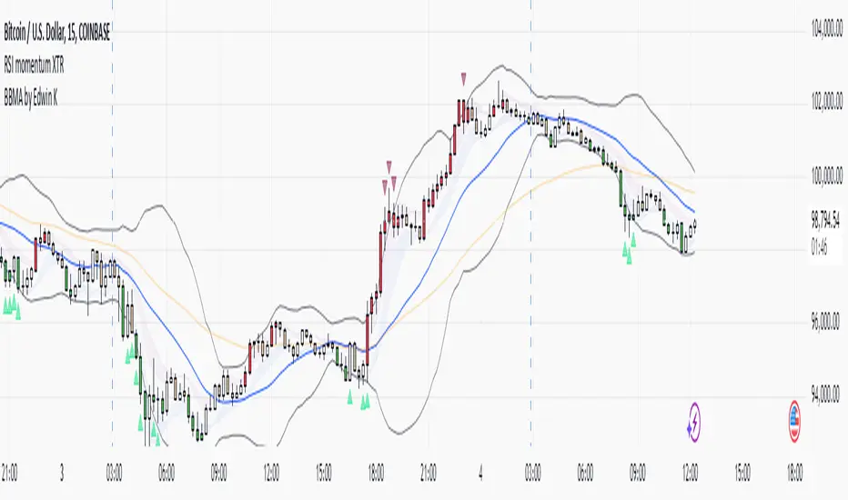
RSI XTR with selective candle color by Edwin KThis tradingView indicator named "RSI XTR with selective candle color", which modifies the candle colors on the chart based on RSI (Relative Strength Index) conditions. Here's how it works:
- rsiPeriod: Defines the RSI calculation period (default = 5).
- rsiOverbought: RSI level considered overbought (default = 70).
- rsiOversold: RSI level considered oversold (default = 30).
- These values can be modified by the user in the settings.
RSI Calculation
- Computes the RSI value using the ta.rsi() function on the closing price (close).
- The RSI is a momentum indicator that measures the magnitude of recent price changes.
Conditions for Candle Coloring
- when the RSI is above the overbought level.
- when the RSI is below the oversold level.
How It Works in Practice
- When the RSI is above 70 (overbought) → Candles turn red.
- When the RSI is below 30 (oversold) → Candles turn green.
- If the RSI is between 30 and 70, the candle keeps its default color.
This helps traders quickly spot potential reversal zones based on RSI momentum.
Search in scripts for "价格在30元内股票"
Relative Strength Index With Range ZoneRSI (Relative Strength Index) with 45-55 Range Zone
1. Introduction and Historical Background
The Relative Strength Index (RSI) is a momentum indicator developed in 1978 by J. Welles Wilder Jr. It measures the speed and magnitude of price changes to assess overbought and oversold conditions of an asset. This widely used oscillator ranges between 0 and 100.
Historically, the RSI was mainly used to detect trend reversals by identifying extreme levels: above 70 (overbought) and below 30 (oversold). However, its application has evolved, and new approaches refine its interpretation, such as adding a 45-55 neutral zone to identify consolidation (range) periods.
2. RSI Calculation
The RSI is calculated using the following formula:
RSI=100−(1001+RS)RSI=100−(1+RS100)
Where:
RS=Average gain over N periodsAverage loss over N periodsRS=Average loss over N periodsAverage gain over N periods
• RS (Relative Strength) is the ratio between the average gains and the average losses over N periods (typically 14 periods).
• Gains and losses are calculated based on daily price variations.
Example calculation with a 14-day period:
1. Compute daily gains and losses.
2. Take an exponential or simple moving average of these values over 14 days.
3. Apply the formula to get the RSI value.
3. Classic RSI Usage
The RSI is typically interpreted as follows:
• RSI > 70: Overbought → Possible correction or bearish reversal.
• RSI < 30: Oversold → Possible rebound or bullish reversal.
• RSI between 50 and 70: Bullish momentum.
• RSI between 30 and 50: Bearish momentum.
4. Adding the 45-55 Zone to Identify Range Phases
Adding a neutral zone between 45 and 55 helps identify consolidation periods, when price moves sideways without a strong trend.
• RSI between 45 and 55: The market is in a range, meaning neither buyers nor sellers dominate.
• RSI breaking out of this zone:
o Above 55: Indicates the start of a bullish trend.
o Below 45: Indicates the start of a bearish trend.
This zone is particularly useful for:
• Avoiding false signals by waiting for trend confirmation.
• Identifying ranging markets, favoring range trading strategies (buying at support, selling at resistance).
• Filtering trend-based entries, waiting for the RSI to exit the 45-55 zone.
5. Trading Strategies Using RSI with the 45-55 Range Zone
1. Range Trading:
• When the RSI oscillates between 45 and 55, it signals a lack of strong trend.
• Strategy:
o Identify a support and resistance level.
o Buy near support when the RSI touches 45.
o Sell near resistance when the RSI touches 55.
2. Breakout Trading:
• If the RSI exits the 45-55 zone:
o Above 55 → Buy (start of a bullish trend).
o Below 45 → Sell (start of a bearish trend).
• This breakout can be used as a confirmed entry signal.
3. Confirmation with Divergences:
• A bullish divergence (price making lower lows while RSI makes higher lows) is more relevant if the RSI moves above 55.
• A bearish divergence (price making higher highs while RSI makes lower highs) is stronger if the RSI drops below 45.
6. Conclusion
The RSI is a powerful tool for analyzing price momentum. Adding a 45-55 zone enhances its usage by clearly distinguishing:
• Consolidation phases (range markets).
• Trend beginnings when RSI breaks out of this range.
This approach improves RSI reliability by filtering out false signals and allowing traders to adapt their strategy based on market conditions.
Gold Pro StrategyHere’s the strategy description in a chat format:
---
**Gold (XAU/USD) Trend-Following Strategy**
This **trend-following strategy** is designed for trading gold (XAU/USD) by combining moving averages, MACD momentum indicators, and RSI filters to capture sustained trends while managing volatility risks. The strategy uses volatility-adjusted stops to protect gains and prevent overexposure during erratic price movements. The aim is to take advantage of trending markets by confirming momentum and ensuring entries are not made at extreme levels.
---
**Key Components**
1. **Trend Identification**
- **50 vs 200 EMA Crossover**
- **Bullish Trend:** 50 EMA crosses above 200 EMA, and the price closes above the 200 EMA
- **Bearish Trend:** 50 EMA crosses below 200 EMA, and the price closes below the 200 EMA
2. **Momentum Confirmation**
- **MACD (12,26,9)**
- **Buy Signal:** MACD line crosses above the signal line
- **Sell Signal:** MACD line crosses below the signal line
- **RSI (14 Period)**
- **Bullish Zone:** RSI between 50-70 to avoid overbought conditions
- **Bearish Zone:** RSI between 30-50 to avoid oversold conditions
3. **Entry Criteria**
- **Long Entry:** Bullish trend, MACD bullish crossover, and RSI between 50-70
- **Short Entry:** Bearish trend, MACD bearish crossover, and RSI between 30-50
4. **Exit & Risk Management**
- **ATR Trailing Stops (14 Period):**
- Initial Stop: 3x ATR from entry price
- Trailing Stop: Adjusts to lock in profits as price moves favorably
- **Position Sizing:** 100% of equity per trade (high-risk strategy)
---
**Key Logic Flow**
1. **Trend Filter:** Use the 50/200 EMA relationship to define the market's direction
2. **Momentum Confirmation:** Confirm trend momentum with MACD crossovers
3. **RSI Validation:** Ensure RSI is within non-extreme ranges before entering trades
4. **Volatility-Based Risk Management:** Use ATR stops to manage market volatility
---
**Visual Cues**
- **Blue Line:** 50 EMA
- **Red Line:** 200 EMA
- **Green Triangles:** Long entry signals
- **Red Triangles:** Short entry signals
---
**Strengths**
- **Clear Trend Focus:** Avoids counter-trend trades
- **RSI Filter:** Prevents entering overbought or oversold conditions
- **ATR Stops:** Adapts to gold’s inherent volatility
- **Simple Rules:** Easy to follow with minimal inputs
---
**Weaknesses & Risks**
- **Infrequent Signals:** 50/200 EMA crossovers are rare
- **Potential Missed Opportunities:** Strict RSI criteria may miss some valid trends
- **Aggressive Position Sizing:** 100% equity allocation can lead to large drawdowns
- **No Profit Targets:** Relies on trailing stops rather than defined exit targets
---
**Performance Profile**
| Metric | Expected Range |
|----------------------|---------------------|
| Annual Trades | 4-8 |
| Win Rate | 55-65% |
| Max Drawdown | 25-35% |
| Profit Factor | 1.8-2.5 |
---
**Optimization Recommendations**
1. **Increase Trade Frequency**
Adjust the EMAs to shorter periods:
- `emaFastLen = input.int(30, "Fast EMA")`
- `emaSlowLen = input.int(150, "Slow EMA")`
2. **Relax RSI Filters**
Adjust the RSI range to:
- `rsiBullish = rsi > 45 and rsi < 75`
- `rsiBearish = rsi < 55 and rsi > 25`
3. **Add Profit Targets**
Introduce a profit target at 1.5% above entry:
```pine
strategy.exit("Long Exit", "Long",
stop=longStopPrice,
profit=close*1.015, // 1.5% target
trail_offset=trailOffset)
```
4. **Reduce Position Sizing**
Risk a smaller percentage per trade:
- `default_qty_value=25`
---
**Best Use Case**
This strategy excels in **strong trending markets** such as gold rallies during economic or geopolitical crises. However, during sideways or choppy market conditions, the strategy might require manual intervention to avoid false signals. Additionally, integrating fundamental analysis—like monitoring USD weakness or geopolitical risks—can enhance its effectiveness.
---
This strategy offers a balanced approach for trading gold, combining trend-following principles with risk management tailored to the volatility of the market.

MA RSI MACD Signal SuiteThis Pine Script™ is designed for use in Trading View and generates trading signals based on moving average (MA) crossovers, RSI (Relative Strength Index) signals, and MACD (Moving Average Convergence Divergence) indicators. It provides visual markers on the chart and can be configured to suit various trading strategies.
1. Indicator Overview
The indicator includes signals for:
Moving Averages (MA): It tracks crossovers between different types of moving averages.
RSI: Signals based on RSI crossing certain levels or its signal line.
MACD: Buy and sell signals generated by MACD crossovers.
2. Inputs and Customization
Moving Averages (MAs):
You can customize up to 6 moving averages with different types, lengths, and colors.
MA Type: Choose from different types of moving averages:
SMA (Simple Moving Average)
EMA (Exponential Moving Average)
HMA (Hull Moving Average)
SMMA (RMA) (Smoothed Moving Average)
WMA (Weighted Moving Average)
VWMA (Volume Weighted Moving Average)
T3, DEMA, TEMA
Source: Select the price to base the MA on (e.g., close, open, high, low).
Length: Define the number of periods for each moving average.
Examples:
MA1: Exponential Moving Average (EMA) with a period of 9
MA2: Exponential Moving Average (EMA) with a period of 21
RSI Settings:
RSI is calculated based on a user-defined period and is used to identify potential overbought or oversold conditions.
RSI Length: Lookback period for RSI (default 14).
Overbought Level: Defines the overbought threshold for RSI (default 70).
Oversold Level: Defines the oversold threshold for RSI (default 30).
You can also adjust the smoothing for the RSI signal line and customize when to trigger buy and sell signals based on the RSI crossing these levels.
MACD Settings:
MACD is used for identifying changes in momentum and trends.
Fast Length: The period for the fast moving average (default 12).
Slow Length: The period for the slow moving average (default 26).
Signal Length: The period for the signal line (default 9).
Smoothing Method: Choose between SMA or EMA for both the MACD and the signal line.
3. Signal Logic
Moving Average (MA) Crossover Signals:
Crossover: A bullish signal is generated when a fast MA crosses above a slow MA.
Crossunder: A bearish signal is generated when a fast MA crosses below a slow MA.
The crossovers are plotted with distinct colors, and the chart will display markers for these crossover events.
RSI Signals:
Oversold Crossover: A bullish signal when RSI crosses over its signal line below the oversold level (30).
Overbought Crossunder: A bearish signal when RSI crosses under its signal line above the overbought level (70).
RSI signals are divided into:
Aggressive (Early) Entries: Signals when RSI is crossing the oversold/overbought levels.
Conservative Entries: Signals when RSI confirms a reversal after crossing these levels.
MACD Signals:
Buy Signal: Generated when the MACD line crosses above the signal line (bullish crossover).
Sell Signal: Generated when the MACD line crosses below the signal line (bearish crossunder).
Additionally, the MACD histogram is used to identify momentum shifts:
Rising to Falling Histogram: Alerts when the MACD histogram switches from rising to falling.
Falling to Rising Histogram: Alerts when the MACD histogram switches from falling to rising.
4. Visuals and Alerts
Plotting:
The script plots the following on the price chart:
Moving Averages (MA): The selected MAs are plotted as lines.
Buy/Sell Shapes: Triangular markers are displayed for buy and sell signals generated by RSI and MACD.
Crossover and Crossunder Markers: Crosses are shown when two MAs crossover or crossunder.
Alerts:
Alerts can be configured based on the following conditions:
RSI Signals: Alerts for oversold or overbought crossover and crossunder events.
MACD Signals: Alerts for MACD line crossovers or momentum shifts in the MACD histogram.
Alerts are triggered when specific conditions are met, such as:
RSI crosses over or under the oversold/overbought levels.
MACD crosses the signal line.
Changes in the MACD histogram.
5. Example Usage
1. Trend Reversal Setup:
Buy Signal: Use the RSI oversold crossover and MACD bullish crossover to identify potential entry points in a downtrend.
Sell Signal: Use the RSI overbought crossunder and MACD bearish crossunder to identify potential exit points or short entries in an uptrend.
2. Momentum Strategy:
Combine MACD and RSI signals to identify the strength of a trend. Use MACD histogram analysis and RSI levels for confirmation.
3. Moving Average Crossover Strategy:
Focus on specific MA crossovers, such as the 9-period EMA crossing above the 21-period EMA, for buy signals. When a longer-term MA (e.g., 50-period) crosses a shorter-term MA, it may indicate a strong trend change.
6. Alerts Conditions
The script includes several alert conditions, which can be triggered and customized based on the user’s preferences:
RSI Oversold Crossover: Alerts when RSI crosses over the signal line below the oversold level (30).
RSI Overbought Crossunder: Alerts when RSI crosses under the signal line above the overbought level (70).
MACD Buy/Sell Crossover: Alerts when the MACD line crosses the signal line for a buy or sell signal.
7. Conclusion
This script is highly customizable and can be adjusted to suit different trading strategies. By combining MAs, RSI, and MACD, traders can gain multiple perspectives on the market, enhancing their ability to identify potential buy and sell opportunities.

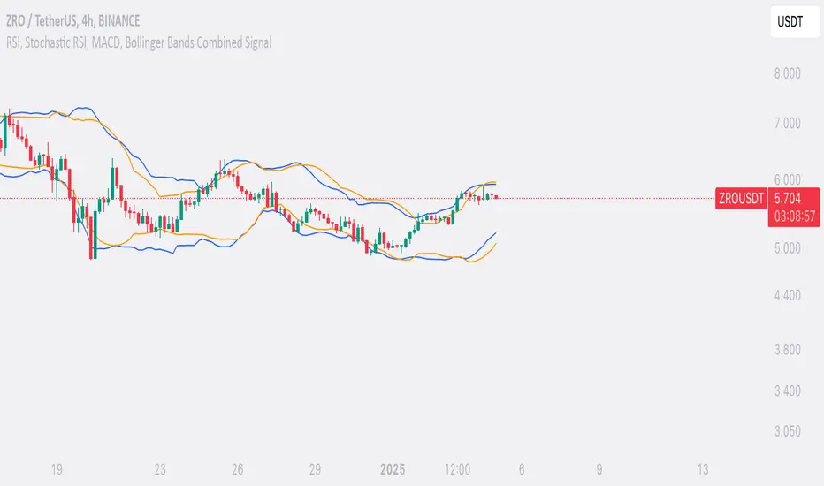
SufinBDThis TradingView script combines RSI, Stochastic RSI, MACD, and Bollinger Bands to generate Buy and Sell signals on two different timeframes: 4-hour (4H) and Daily (1D). The strategy aims to provide entry and exit points based on a multi-indicator confirmation approach, helping traders make more informed decisions.
Features:
RSI (Relative Strength Index):
Measures the speed and change of price movements.
The script looks for oversold conditions (RSI below 30) for buy signals and overbought conditions (RSI above 70) for sell signals.
Stochastic RSI:
Measures the level of RSI relative to its high-low range over a given period.
A Stochastic RSI below 0.2 indicates oversold conditions, and a value above 0.8 indicates overbought conditions.
It helps identify overbought and oversold conditions in a more precise manner than regular RSI.
MACD (Moving Average Convergence Divergence):
A trend-following momentum indicator that shows the relationship between two moving averages of a security's price.
The MACD line crossing above the Signal line generates bullish signals, and vice versa for bearish signals.
Bollinger Bands:
A volatility indicator that consists of a middle band (SMA of price), an upper band, and a lower band.
When the price is below the lower band, it signals potential buy opportunities, while prices above the upper band signal potential sell opportunities.
Timeframe Usage:
The script calculates indicators for both the 4-hour (4H) and Daily (1D) timeframes.
The combined signals from these two timeframes are used to generate Buy and Sell alerts.
Buy Signal:
A Buy signal is generated when all of the following conditions are met:
RSI on both 4H and 1D is below 30 (oversold conditions).
Stochastic RSI on both timeframes is below 0.2.
The MACD line is above the Signal line on both timeframes.
The price is below the lower Bollinger Band on both the 4H and 1D charts.
Sell Signal:
A Sell signal is generated when all of the following conditions are met:
RSI on both 4H and 1D is above 70 (overbought conditions).
Stochastic RSI on both timeframes is above 0.8.
The MACD line is below the Signal line on both timeframes.
The price is above the upper Bollinger Band on both the 4H and 1D charts.
Visuals:
Buy signals are marked with green labels below the bars.
Sell signals are marked with red labels above the bars.
Bollinger Bands are displayed on the chart with the upper and lower bands marked in blue (for 4H) and orange (for 1D).
Purpose:
This script aims to provide more reliable buy/sell signals by combining indicators across multiple timeframes. It is ideal for traders who want to use multiple confirmation points before entering or exiting a trade.
How to Use:
Apply the script to any chart on TradingView.
Look for Buy and Sell signals that meet the conditions above.
You can adjust the timeframe (e.g., 4H or 1D) based on your trading strategy.
This script can be used for intraday trading, swing trading, or position trading depending on your preferred timeframes.
Example of Signal Interpretation:
Buy Signal:
If all conditions are met (e.g., RSI is under 30, Stochastic RSI is under 0.2, MACD is bullish, and price is below the lower Bollinger Band on both the 4-hour and daily charts), the script will show a green "BUY" label below the price bar.
Sell Signal:
If all conditions are met (e.g., RSI is over 70, Stochastic RSI is over 0.8, MACD is bearish, and price is above the upper Bollinger Band on both timeframes), the script will show a red "SELL" label above the price bar.
This combination of indicators offers a multi-layered confirmation approach, which aims to reduce the risk of false signals and increase the reliability of your trading decisions.
Binary Options Pro Helper By Himanshu AgnihotryThe Binary Options Pro Helper is a custom indicator designed specifically for one-minute binary options trading. This tool combines technical analysis methods like moving averages, RSI, Bollinger Bands, and pattern recognition to provide precise Buy and Sell signals. It also includes a time-based filter to ensure trades are executed only during optimal market conditions.
Features:
Moving Averages (EMA):
Uses short-term (7-period) and long-term (21-period) EMA crossovers for trend detection.
RSI-Based Signals:
Identifies overbought/oversold conditions for entry points.
Bollinger Bands:
Highlights market volatility and potential reversal zones.
Chart Pattern Recognition:
Detects double tops (sell signals) and double bottoms (buy signals).
Time-Based Filter:
Trades only within specified hours (e.g., 9:30 AM to 11:30 AM) to avoid unnecessary noise.
Visual Signals:
Plots buy and sell markers directly on the chart for ease of use.
How to Use:
Setup:
Add this script to your TradingView chart and select a 1-minute timeframe.
Signal Interpretation:
Buy Signal: Triggered when EMA crossover occurs, RSI is oversold (<30), and a double bottom pattern is detected.
Sell Signal: Triggered when EMA crossover occurs, RSI is overbought (>70), and a double top pattern is detected.
Timing:
Ensure trades are executed only during the specified time window for better accuracy.
Best Practices:
Use this indicator alongside fundamental analysis or market sentiment.
Test it thoroughly with historical data (backtesting) and in a demo account before live trading.
Adjust parameters (e.g., EMA periods, RSI thresholds) based on your trading style.

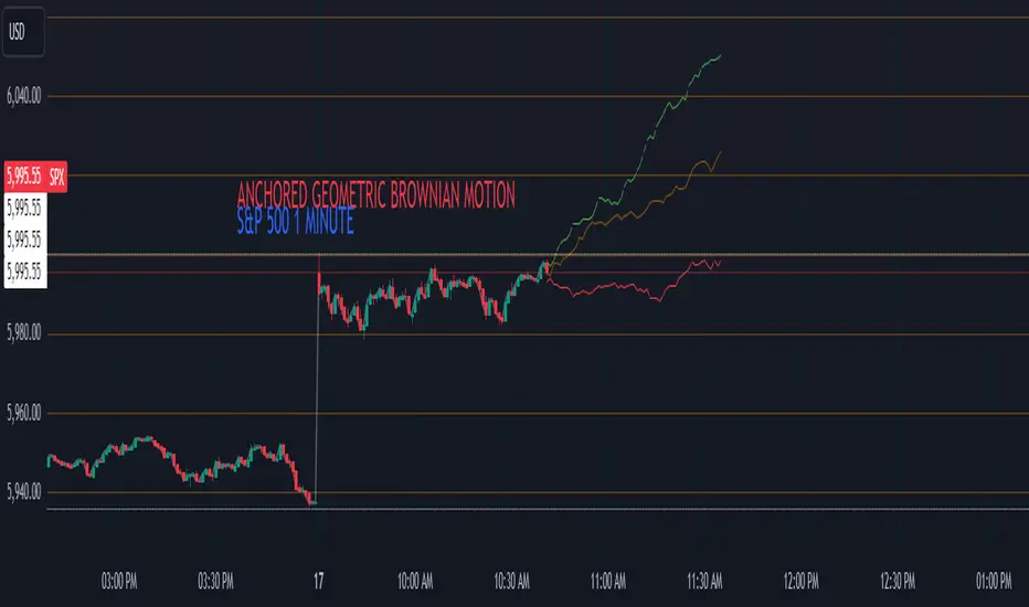
Anchored Geometric Brownian Motion Projections w/EVAnchored GBM (Geometric Brownian Motion) Projections + EV & Confidence Bands
Version: Pine Script v6
Overlay: Yes
Author:
Published On:
Overview
The Anchored GBM Projections + EV & Confidence Bands indicator leverages the Geometric Brownian Motion (GBM) model to project future price movements based on historical data. By simulating multiple potential future price paths, it provides traders with insights into possible price trajectories, their expected values, and confidence intervals. Additionally, it offers a "Mean of EV" (EV of EV) line, representing the running average of expected values across the projection period.
Key Features
Anchor Time Setup:
Define a specific point in time from which the projections commence.
By default, it uses the current bar's timestamp but can be customized.
Projection Parameters:
Projection Candles (Bars): Determines the number of future bars (time periods) to project.
Number of Simulations: Specifies how many GBM paths to simulate, ensuring statistical relevance via the Central Limit Theorem (CLT).
Display Toggles:
Simulation Lines: Visual representation of individual GBM simulation paths.
Expected Value (EV) Line: The average price across all simulations at each projection bar.
Upper & Lower Confidence Bands: 95% confidence intervals indicating potential price boundaries.
EV of EV Line: Running average of EV values, providing a smoothed central tendency across the projection period. Additionally, this line often acts as an indicator of trend direction.
Visualization:
Clear and distinguishable lines with customizable colors and styles.
Overlayed on the price chart for direct comparison with actual price movements.
Mathematical Foundation
Geometric Brownian Motion (GBM):
Definition: GBM is a continuous-time stochastic process used to model stock prices. It assumes that the logarithm of the stock price follows a Brownian motion with drift.
Equation:
S(t)=S0⋅e(μ−12σ2)t+σW(t)
S(t)=S0⋅e(μ−21σ2)t+σW(t) Where:
S(t)S(t) = Stock price at time tt
S0S0 = Initial stock price
μμ = Drift coefficient (average return)
σσ = Volatility coefficient (standard deviation of returns)
W(t)W(t) = Wiener process (standard Brownian motion)
Drift (μμ) and Volatility (σσ):
Drift (μμ) represents the expected return of the stock.
Volatility (σσ) measures the stock's price fluctuation intensity.
Central Limit Theorem (CLT):
Principle: With a sufficiently large number of independent simulations, the distribution of the sample mean (EV) approaches a normal distribution, regardless of the underlying distribution.
Application: Ensures that the EV and confidence bands are statistically reliable.
Expected Value (EV) and Confidence Bands:
EV: The mean price across all simulations at each projection bar.
Confidence Bands: Range within which the actual price is expected to lie with a specified probability (e.g., 95%).
EV of EV (Mean of Sample Means):
Definition: Represents the running average of EV values across the projection period, offering a smoothed central tendency.
Methodology
Anchor Time Setup:
The indicator starts projecting from a user-defined Anchor Time. If not customized, it defaults to the current bar's timestamp.
Purpose: Allows users to analyze projections from a specific historical point or the latest market data.
Calculating Drift and Volatility:
Returns Calculation: Computes the logarithmic returns from the Anchor Time to the current bar.
returns=ln(StSt−1)
returns=ln(St−1St)
Drift (μμ): Calculated as the simple moving average (SMA) of returns over the period since the Anchor Time.
Volatility (σσ): Determined using the standard deviation (stdev) of returns over the same period.
Simulation Generation:
Number of Simulations: The user defines how many GBM paths to simulate (e.g., 30).
Projection Candles: Determines the number of future bars to project (e.g., 12).
Process:
For each simulation:
Start from the current close price.
For each projection bar:
Generate a random number zz from a standard normal distribution.
Calculate the next price using the GBM formula:
St+1=St⋅e(μ−12σ2)+σz
St+1=St⋅e(μ−21σ2)+σz
Store the projected price in an array.
Expected Value (EV) and Confidence Bands Calculation:
EV Path: At each projection bar, compute the mean of all simulated prices.
Variance and Standard Deviation: Calculate the variance and standard deviation of simulated prices to determine the confidence intervals.
Confidence Bands: Using the standard normal z-score (1.96 for 95% confidence), establish upper and lower bounds:
Upper Band=EV+z⋅σEV
Upper Band=EV+z⋅σEV
Lower Band=EV−z⋅σEV
Lower Band=EV−z⋅σEV
EV of EV (Running Average of EV Values):
Calculation: For each projection bar, compute the average of all EV values up to that bar.
EV of EV =1j+1∑k=0jEV
EV of EV =j+11k=0∑jEV
Visualization: Plotted as a dynamic line reflecting the evolving average EV across the projection period.
Visualization Elements
Simulation Lines:
Appearance: Semi-transparent blue lines representing individual GBM simulation paths.
Purpose: Illustrate a range of possible future price trajectories based on current drift and volatility.
Expected Value (EV) Line:
Appearance: Solid orange line.
Purpose: Shows the average projected price at each future bar across all simulations.
Confidence Bands:
Upper Band: Dashed green line indicating the upper 95% confidence boundary.
Lower Band: Dashed red line indicating the lower 95% confidence boundary.
Purpose: Highlight the range within which the price is statistically expected to remain with 95% confidence.
EV of EV Line:
Appearance: Dashed purple line.
Purpose: Displays the running average of EV values, providing a smoothed trend of the central tendency across the projection period. As the mean of sample means it approximates the population mean (i.e. the trend since the anchor point.)
Current Price:
Appearance: Semi-transparent white line.
Purpose: Serves as a reference point for comparing actual price movements against projected paths.
Usage Instructions
Configuring User Inputs:
Anchor Time:
Set to a specific timestamp to start projections from a historical point or leave it as default to use the current bar's time.
Projection Candles (Bars):
Define the number of future bars to project (e.g., 12). Adjust based on your trading timeframe and analysis needs.
Number of Simulations:
Specify the number of GBM paths to simulate (e.g., 30). Higher numbers yield more accurate EV and confidence bands but may impact performance.
Display Toggles:
Show Simulation Lines: Toggle to display or hide individual GBM simulation paths.
Show Expected Value Line: Toggle to display or hide the EV path.
Show Upper Confidence Band: Toggle to display or hide the upper confidence boundary.
Show Lower Confidence Band: Toggle to display or hide the lower confidence boundary.
Show EV of EV Line: Toggle to display or hide the running average of EV values.
Managing TradingView's Object Limits:
Understanding Limits:
TradingView imposes a limit on the number of graphical objects (e.g., lines) that can be rendered. High values for projection candles and simulations can quickly consume these limits. TradingView appears to only allow a total of 55 candles to be projected, so if you want to see two complete lines, you would have to set the projection length to 27: since 27 * 2 = 54 and 54 < 55.
Optimizing Performance:
Use Toggles: Enable only the necessary visual elements. For instance, disable simulation lines and confidence bands when focusing on the EV and EV of EV lines. You can also use the maximum projection length of 55 with the lower limit confidence band as the only line, visualizing a long horizon for your risk.
Adjust Parameters: Lower the number of projection candles or simulations to stay within object limits without compromising essential insights.
Interpreting the Indicator:
Simulation Lines (Blue):
Represent individual potential future price paths based on GBM. A wider spread indicates higher volatility.
Expected Value (EV) Line (Goldenrod):
Shows the mean projected price at each future bar, providing a central trend.
Confidence Bands (Green & Red):
Indicate the statistical range (95% confidence) within which the price is expected to remain.
EV of EV Line (Dotted Line - Goldenrod):
Reflects the running average of EV values, offering a smoothed perspective of expected price trends over the projection period.
Current Price (White):
Serves as a benchmark for assessing how actual prices compare to projected paths.
Practical Applications
Risk Management:
Confidence Bands: Help in identifying potential support and resistance levels based on statistical confidence intervals.
EV Path: Assists in setting realistic target prices and stop-loss levels aligned with projected expectations.
Trend Analysis:
EV of EV Line: Offers a smoothed trendline, aiding in identifying overarching market directions amidst price volatility. Indicative of the population mean/overall trend of the data since your anchor point.
Scenario Planning:
Simulation Lines: Enable traders to visualize multiple potential outcomes, fostering better decision-making under uncertainty.
Performance Evaluation:
Comparing Actual vs. Projected Prices: Assess how actual price movements align with projected scenarios, refining trading strategies over time.
Mathematical and Statistical Insights
Simulation Integrity:
Independence: Each simulation path is generated independently, ensuring unbiased and diverse projections.
Randomness: Utilizes a Gaussian random number generator to introduce variability in diffusion terms, mimicking real market randomness.
Statistical Reliability:
Central Limit Theorem (CLT): By simulating a sufficient number of paths (e.g., 30), the sample mean (EV) converges to the population mean, ensuring reliable EV and confidence band calculations.
Variance Calculation: Accurate computation of variance from simulation data ensures precise confidence intervals.
Dynamic Projections:
Running Average (EV of EV): Provides a cumulative perspective, allowing traders to observe how the average expectation evolves as the projection progresses.
Customization and Enhancements
Adjustable Parameters:
Tailor the projection length and simulation count to match your trading style and analysis depth.
Visual Customization:
Modify line colors, styles, and transparency to enhance clarity and fit chart aesthetics.
Extended Statistical Metrics:
Future iterations can incorporate additional metrics like median projections, skewness, or alternative confidence intervals.
Dynamic Recalculation:
Implement logic to automatically update projections as new data becomes available, ensuring real-time relevance.
Performance Considerations
Object Count Management:
High simulation counts and extended projection periods can lead to a significant number of graphical objects, potentially slowing down chart performance.
Solution: Utilize display toggles effectively and optimize projection parameters to balance detail with performance.
Computational Efficiency:
The script employs efficient array handling and conditional plotting to minimize unnecessary computations and object creation.
Conclusion
The Anchored GBM Projections + EV & Confidence Bands indicator is a robust tool for traders seeking to forecast potential future price movements using statistical models. By integrating Geometric Brownian Motion simulations with expected value calculations and confidence intervals, it offers a comprehensive view of possible market scenarios. The addition of the "EV of EV" line further enhances analytical depth by providing a running average of expected values, aiding in trend identification and strategic decision-making.
Hope it helps!
Wickiness IndexWickiness Index - Detect Indecision and Trend Exhaustion
The Wickiness Index is a versatile technical indicator designed to measure the proportion of wicks (upper and lower shadows) relative to the total range of price bars over a specified lookback period. It provides insights into market indecision, reversals, and trend exhaustion by analyzing the structural composition of candlesticks. The indicator calculates the lengths of upper and lower wicks along with the body of each candlestick. Each bar's wick length is expressed as a percentage of the total range (High - Low). The ratio is scaled to 0–100, where 100 represents entirely wicks with no body (indicating pure indecision) and 0 represents no wicks with only body (indicating strong directional movement). These values are then averaged over the lookback period (default = 5 bars) to provide a smoothed representation of wickiness, reducing noise and highlighting trends.
A high value, especially above 70, suggests indecision or potential reversals, as candlesticks dominated by wicks often appear near tops or bottoms. Conversely, low values below 30 indicate trend strength and strong momentum, useful for spotting breakouts and trend continuation. Mid-range values between 30 and 70 often indicate consolidation phases or gradual transitions between trends. Traders can adjust the lookback period to match their trading style, with shorter periods offering faster responses and longer periods providing smoother trends.
This indicator is particularly useful for trend reversal detection, breakout confirmation, and volatility filtering. It scales effectively across all timeframes, making it suitable for both intraday traders and long-term investors. When combined with volume analysis or trend-following indicators, the Wickiness Index can further strengthen trade signals. The visual design includes a blue line for the index and horizontal reference lines at 30 and 70, allowing for quick and intuitive interpretation.
The Wickiness Index offers a unique perspective on market sentiment and price action behavior, providing traders with valuable insights into potential turning points, momentum shifts, and market indecision. It is a powerful tool for improving decision-making in volatile markets and identifying areas where price trends may weaken or reverse.

Gold Trade Setup Strategy
Title: Profitable Gold Setup Strategy with Adaptive Moving Average & Supertrend
Introduction:
This trading strategy for Gold (XAU/USD) combines the Adaptive Moving Average (AMA) and Supertrend, tailored for high-probability setups during specific trading hours. The AMA identifies the trend, while the Supertrend confirms entry and exit points. The strategy is optimized for swing and intraday traders looking to capitalize on Gold’s price movements with precise trade timing.
Strategy Components:
1. Adaptive Moving Average (AMA):
• Reacts dynamically to market conditions, filtering noise in choppy markets.
• Serves as the primary trend indicator.
2. Supertrend:
• Confirms entry signals with clear buy and sell levels.
• Acts as a trailing stop-loss to protect profits.
Trading Rules:
Trading Hours:
• Only take trades between 8:30 AM and 10:30 PM IST.
• Avoid trading outside these hours to reduce noise and low-volume setups.
Buy Setup:
1. Trend Confirmation: The Adaptive Moving Average (AMA) must be green.
2. Signal Confirmation: The Supertrend should turn green after the AMA is green.
3. Trigger: Take the trade when the high of the trigger candle (the candle that turned Supertrend green) is broken.
Sell Setup (Optional if included):
• Reverse the rules for a short trade: AMA and Supertrend should both indicate bearish conditions (red), and take the trade when the low of the trigger candle is broken.
Stop-Loss and Targets:
• Place the stop-loss at the low of the trigger candle for long trades.
• Set a 1:2 risk-reward ratio or use the Supertrend line as a trailing stop-loss.
Timeframes:
• Recommended timeframes: 1H, 4H, or Daily for swing trading.
• For intraday trading, use 15-minute or 30-minute charts.
Why This Strategy Works:
• Combines trend-following (AMA) with momentum-based entries (Supertrend).
• Focused trading hours filter out low-probability setups.
• Provides precise entry, stop-loss, and target levels for disciplined trading.
Conclusion:
This Gold Setup Strategy is designed for traders seeking a structured approach to trading Gold. Follow the rules strictly, backtest the strategy extensively, and share your results. Let’s master the Gold market together!
Tags: #Gold #XAUUSD #SwingTrading #Intraday #Supertrend #AMA #TechnicalAnalysis #GoldStrategy
Support/Resistance
Custom Moving Average Indicator with MACD, RSI, and Support/Resistance
This indicator is designed to help traders make informed trading decisions by integrating several technical indicators, including moving averages, the Relative Strength Index (RSI), and the Moving Average Convergence Divergence (MACD).
Key Features:
Moving Averages:
This indicator uses simple moving averages (SMAs) for several periods (4, 18, 66, 89, 632, 1000, 1500, 2000, and 3000 bars). This helps to identify the overall trend of the price and potential support and resistance levels.
The color of each moving average line is dynamically changed based on the closing price's position relative to the average; it turns red if the price is above the average and green if the price is below.
Relative Strength Index (RSI):
The RSI is calculated for a 14-bar period, which is a measure of overbought or oversold conditions.
An RSI value above 70 indicates an overbought condition, while a value below 30 indicates an oversold condition.
MACD:
The MACD is calculated using a fast length of 12, a slow length of 26, and a signal length of 9. Crossovers between the MACD line and the signal line indicate momentum shifts.
A crossover of the MACD line above the signal line suggests a potential buy signal, while a crossover below indicates a potential sell signal.
Buy and Sell Signals:
Buy Signal: Triggered when the MACD line crosses above the signal line, the RSI is below 30, the MACD is above 0, and there is high volume.
Sell Signal: Triggered when the MACD line crosses below the signal line, the RSI is above 70, the MACD is below 0, and there is high volume.
Alerts:
The indicator includes alerts that are triggered when buy and sell signals occur, helping traders respond quickly to market opportunities.
How to Trade Using the Indicator (continued):
Trading on Buy Signals:
Look for buy signals when the MACD line crosses above the signal line. Ensure that the RSI is below 30, indicating there is a potential for price recovery from an oversold condition.
Confirm that the volume is above the average, which indicates strong market participation and adds validity to the trade.
Trading on Sell Signals:
Search for sell signals when the MACD line crosses below the signal line. Check that the RSI is above 70 to confirm an overbought condition, implying the price may decline.
As with buy signals, ensure that volume is high to validate the strength of the sell signal.
Risk Management:
Use stop-loss orders to protect your capital. Establish an initial loss threshold based on your risk management strategy.
Continuously monitor the market and new signals and adjust your approach according to your market analysis.
Conclusion:
This combined indicator helps traders make informed decisions by relying on a set of technical tools. To achieve the best results, ensure you integrate the analysis from these indicators with your trading strategies and other techniques.
Feel free to use this explanation as an introduction or guide to inform traders on how to effectively use the indicator. If you have any more questions or need further details, don't hesitate to ask!

ATT + Key Levels with SessionsKey Features:
ATT Turning Point Numbers:
This input allows the user to define specific numbers (e.g., "3,11,17,29,41,47,53,59") that mark turning points in price action, which are checked using the bar_index modulo 60. If the current bar index matches one of these turning points, it triggers potential buy or sell signals.
RSI (Relative Strength Index):
The RSI is calculated based on a user-defined period (rsi_period), typically 14, and used to indicate overbought or oversold conditions. The script defines overbought (70) and oversold (30) levels, which are used to filter buy or sell signals.
Session Times:
The script includes predefined session times for major trading markets:
New York: From 9:30 AM EST to 4:00 PM EST.
London: From 8:00 AM GMT to 4:30 PM GMT.
Asia: From 12:00 AM GMT to 9:00 AM GMT.
These session times are used to restrict the buy and sell signals to specific market sessions.
Key Levels:
The script calculates and plots key market levels for the current day and week:
Daily High and Low: The highest and lowest prices of the current day.
Weekly High and Low: The highest and lowest prices of the current week.
These levels are plotted with different colors for visual reference.
Signal Logic:
Buy Signal: Triggered when the current bar is a turning point (according to the ATT model), the RSI is below the oversold threshold, and the current time is within the active session times (New York, London, or Asia).
Sell Signal: Triggered when the current bar is a turning point, the RSI is above the overbought threshold, and the current time is within the active session times.
Signal Limitations:
A user-defined limit (max_signals_per_session) controls the maximum number of signals that can be plotted within each session. This prevents excessive signal generation.
Plotting and Background Highlights:
Buy and Sell Signals: The script plots shapes (labels) above or below the bars to indicate buy or sell signals when the conditions are met.
Background Highlight: The background color is highlighted in yellow when the current bar matches one of the defined ATT turning points.
In Summary:
The indicator combines multiple technical factors to generate trading signals:
Turning points in price action (based on custom ATT numbers),
RSI levels (overbought/oversold),
Market session times (New York, London, Asia),
Key price levels (daily and weekly highs and lows).
This combination helps traders identify potential buying and selling opportunities while considering broader market dynamics and limiting the number of signals during each session.

Logarithmic Regression AlternativeLogarithmic regression is typically used to model situations where growth or decay accelerates rapidly at first and then slows over time. Bitcoin is a good example.
𝑦 = 𝑎 + 𝑏 * ln(𝑥)
With this logarithmic regression (log reg) formula 𝑦 (price) is calculated with constants 𝑎 and 𝑏, where 𝑥 is the bar_index .
Instead of using the sum of log x/y values, together with the dot product of log x/y and the sum of the square of log x-values, to calculate a and b, I wanted to see if it was possible to calculate a and b differently.
In this script, the log reg is calculated with several different assumed a & b values, after which the log reg level is compared to each Swing. The log reg, where all swings on average are closest to the level, produces the final 𝑎 & 𝑏 values used to display the levels.
🔶 USAGE
The script shows the calculated logarithmic regression value from historical swings, provided there are enough swings, the price pattern fits the log reg model, and previous swings are close to the calculated Top/Bottom levels.
When the price approaches one of the calculated Top or Bottom levels, these levels could act as potential cycle Top or Bottom.
Since the logarithmic regression depends on swing values, each new value will change the calculation. A well-fitted model could not fit anymore in the future.
Swings are based on Weekly bars. A Top Swing, for example, with Swing setting 30, is the highest value in 60 weeks. Thirty bars at the left and right of the Swing will be lower than the Top Swing. This means that a confirmation is triggered 30 weeks after the Swing. The period will be automatically multiplied by 7 on the daily chart, where 30 becomes 210 bars.
Please note that the goal of this script is not to show swings rapidly; it is meant to show the potential next cycle's Top/Bottom levels.
🔹 Multiple Levels
The script includes the option to display 3 Top/Bottom levels, which uses different values for the swing calculations.
Top: 'high', 'maximum open/close' or 'close'
Bottom: 'low', 'minimum open/close' or 'close'
These levels can be adjusted up/down with a percentage.
Lastly, an "Average" is included for each set, which will only be visible when "AVG" is enabled, together with both Top and Bottom levels.
🔹 Notes
Users have to check the validity of swings; the above example only uses 1 Top Swing for its calculations, making the Top level unreliable.
Here, 1 of the Bottom Swings is pretty far from the bottom level, changing the swing settings can give a more reliable bottom level where all swings are close to that level.
Note the display was set at "Logarithmic", it can just as well be shown as "Regular"
In the example below, the price evolution does not fit the logarithmic regression model, where growth should accelerate rapidly at first and then slows over time.
Please note that this script can only be used on a daily timeframe or higher; using it at a lower timeframe will show a warning. Also, it doesn't work with bar-replay.
🔶 DETAILS
The code gathers data from historical swings. At the last bar, all swings are calculated with different a and b values. The a and b values which results in the smallest difference between all swings and Top/Bottom levels become the final a and b values.
The ranges of a and b are between -20.000 to +20.000, which means a and b will have the values -20.000, -19.999, -19.998, -19.997, -19.996, ... -> +20.000.
As you can imagine, the number of calculations is enormous. Therefore, the calculation is split into parts, first very roughly and then very fine.
The first calculations are done between -20 and +20 (-20, -19, -18, ...), resulting in, for example, 4.
The next set of calculations is performed only around the previous result, in this case between 3 (4-1) and 5 (4+1), resulting in, for example, 3.9. The next set goes even more in detail, for example, between 3.8 (3.9-0.1) and 4.0 (3.9 + 0.1), and so on.
1) -20 -> +20 , then loop with step 1 (result (example): 4 )
2) 4 - 1 -> 4 +1 , then loop with step 0.1 (result (example): 3.9 )
3) 3.9 - 0.1 -> 3.9 +0.1 , then loop with step 0.01 (result (example): 3.93 )
4) 3.93 - 0.01 -> 3.93 +0.01, then loop with step 0.001 (result (example): 3.928)
This ensures complicated calculations with less effort.
These calculations are done at the last bar, where the levels are displayed, which means you can see different results when a new swing is found.
Also, note that this indicator has been developed for a daily (or higher) timeframe chart.
🔶 SETTINGS
Three sets
High/Low
• color setting
• Swing Length settings for 'High' & 'Low'
• % adjustment for 'High' & 'Low'
• AVG: shows average (when both 'High' and 'Low' are enabled)
Max/Min (maximum open/close, minimum open/close)
• color setting
• Swing Length settings for 'Max' & 'Min'
• % adjustment for 'Max' & 'Min'
• AVG: shows average (when both 'Max' and 'Min' are enabled)
Close H/Close L (close Top/Bottom level)
• color setting
• Swing Length settings for 'Close H' & 'Close L'
• % adjustment for 'Close H' & 'Close L'
• AVG: shows average (when both 'Close H' and 'Close L' are enabled)
Show Dashboard, including Top/Bottom levels of the desired source and calculated a and b values.
Show Swings + Dot size

Ensemble Alerts█ OVERVIEW
This indicator creates highly customizable alert conditions and messages by combining several technical conditions into groups , which users can specify directly from the "Settings/Inputs" tab. It offers a flexible framework for building and testing complex alert conditions without requiring code modifications for each adjustment.
█ CONCEPTS
Ensemble analysis
Ensemble analysis is a form of data analysis that combines several "weaker" models to produce a potentially more robust model. In a trading context, one of the most prevalent forms of ensemble analysis is the aggregation (grouping) of several indicators to derive market insights and reinforce trading decisions. With this analysis, traders typically inspect multiple indicators, signaling trade actions when specific conditions or groups of conditions align.
Simplifying ensemble creation
Combining indicators into one or more ensembles can be challenging, especially for users without programming knowledge. It usually involves writing custom scripts to aggregate the indicators and trigger trading alerts based on the confluence of specific conditions. Making such scripts customizable via inputs poses an additional challenge, as it often involves complicated input menus and conditional logic.
This indicator addresses these challenges by providing a simple, flexible input menu where users can easily define alert criteria by listing groups of conditions from various technical indicators in simple text boxes . With this script, you can create complex alert conditions intuitively from the "Settings/Inputs" tab without ever writing or modifying a single line of code. This framework makes advanced alert setups more accessible to non-coders. Additionally, it can help Pine programmers save time and effort when testing various condition combinations.
█ FEATURES
Configurable alert direction
The "Direction" dropdown at the top of the "Settings/Inputs" tab specifies the allowed direction for the alert conditions. There are four possible options:
• Up only : The indicator only evaluates upward conditions.
• Down only : The indicator only evaluates downward conditions.
• Up and down (default): The indicator evaluates upward and downward conditions, creating alert triggers for both.
• Alternating : The indicator prevents alert triggers for consecutive conditions in the same direction. An upward condition must be the first occurrence after a downward condition to trigger an alert, and vice versa for downward conditions.
Flexible condition groups
This script features six text inputs where users can define distinct condition groups (ensembles) for their alerts. An alert trigger occurs if all the conditions in at least one group occur.
Each input accepts a comma-separated list of numbers with optional spaces (e.g., "1, 4, 8"). Each listed number, from 1 to 35, corresponds to a specific individual condition. Below are the conditions that the numbers represent:
1 — RSI above/below threshold
2 — RSI below/above threshold
3 — Stoch above/below threshold
4 — Stoch below/above threshold
5 — Stoch K over/under D
6 — Stoch K under/over D
7 — AO above/below threshold
8 — AO below/above threshold
9 — AO rising/falling
10 — AO falling/rising
11 — Supertrend up/down
12 — Supertrend down/up
13 — Close above/below MA
14 — Close below/above MA
15 — Close above/below open
16 — Close below/above open
17 — Close increase/decrease
18 — Close decrease/increase
19 — Close near Donchian top/bottom (Close > (Mid + HH) / 2)
20 — Close near Donchian bottom/top (Close < (Mid + LL) / 2)
21 — New Donchian high/low
22 — New Donchian low/high
23 — Rising volume
24 — Falling volume
25 — Volume above average (Volume > SMA(Volume, 20))
26 — Volume below average (Volume < SMA(Volume, 20))
27 — High body to range ratio (Abs(Close - Open) / (High - Low) > 0.5)
28 — Low body to range ratio (Abs(Close - Open) / (High - Low) < 0.5)
29 — High relative volatility (ATR(7) > ATR(40))
30 — Low relative volatility (ATR(7) < ATR(40))
31 — External condition 1
32 — External condition 2
33 — External condition 3
34 — External condition 4
35 — External condition 5
These constituent conditions fall into three distinct categories:
• Directional pairs : The numbers 1-22 correspond to pairs of opposing upward and downward conditions. For example, if one of the inputs includes "1" in the comma-separated list, that group uses the "RSI above/below threshold" condition pair. In this case, the RSI must be above a high threshold for the group to trigger an upward alert, and the RSI must be below a defined low threshold to trigger a downward alert.
• Non-directional filters : The numbers 23-30 correspond to conditions that do not represent directional information. These conditions act as filters for both upward and downward alerts. Traders often use non-directional conditions to refine trending or mean reversion signals. For instance, if one of the input lists includes "30", that group uses the "Low relative volatility" condition. The group can trigger an upward or downward alert only if the 7-period Average True Range (ATR) is below the 40-period ATR.
• External conditions : The numbers 31-35 correspond to external conditions based on the plots from other indicators on the chart. To set these conditions, use the source inputs in the "External conditions" section near the bottom of the "Settings/Inputs" tab. The external value can represent an upward, downward, or non-directional condition based on the following logic:
▫ Any value above 0 represents an upward condition.
▫ Any value below 0 represents a downward condition.
▫ If the checkbox next to the source input is selected, the condition becomes non-directional . Any group that uses the condition can trigger upward or downward alerts only if the source value is not 0.
To learn more about using plotted values from other indicators, see this article in our Help Center and the Source input section of our Pine Script™ User Manual.
Group markers
Each comma-separated list represents a distinct group , where all the listed conditions must occur to trigger an alert. This script assigns preset markers (names) to each condition group to make the active ensembles easily identifiable in the generated alert messages and labels. The markers assigned to each group use the format "M", where "M" is short for "Marker" and "x" is the group number. The titles of the inputs at the top of the "Settings/Inputs" tab show these markers for convenience.
For upward conditions, the labels and alert messages show group markers with upward triangles (e.g., "M1▲"). For downward conditions, they show markers with downward triangles (e.g., "M1▼").
NOTE: By default, this script populates the "M1" field with a pre-configured list for a mean reversion group ("2,18,24,28"). The other fields are empty. If any "M*" input does not contain a value, the indicator ignores it in the alert calculations.
Custom alert messages
By default, the indicator's alert message text contains the activated markers and their direction as a comma-separated list. Users can override this message for upward or downward alerts with the two text fields at the bottom of the "Settings/Inputs" tab. When the fields are not empty , the alerts use that text instead of the default marker list.
NOTE: This script generates alert triggers, not the alerts themselves. To set up an alert based on this script's conditions, open the "Create Alert" dialog box, then select the "Ensemble Alerts" and "Any alert() function call" options in the "Condition" tabs. See the Alerts FAQ in our Pine Script™ User Manual for more information.
Condition visualization
This script offers organized visualizations of its conditions, allowing users to inspect the behaviors of each condition alongside the specified groups. The key visual features include:
1) Conditional plots
• The indicator plots the history of each individual condition, excluding the external conditions, as circles at different levels. Opposite conditions appear at positive and negative levels with the same absolute value. The plots for each condition show values only on the bars where they occur.
• Each condition's plot is color-coded based on its type. Aqua and orange plots represent opposing directional conditions, and purple plots represent non-directional conditions. The titles of the plots also contain the condition numbers to which they apply.
• The plots in the separate pane can be turned on or off with the "Show plots in pane" checkbox near the top of the "Settings/Inputs" tab. This input only toggles the color-coded circles, which reduces the graphical load. If you deactivate these visuals, you can still inspect each condition from the script's status line and the Data Window.
• As a bonus, the indicator includes "Up alert" and "Down alert" plots in the Data Window, representing the combined upward and downward ensemble alert conditions. These plots are also usable in additional indicator-on-indicator calculations.
2) Dynamic labels
• The indicator draws a label on the main chart pane displaying the activated group markers (e.g., "M1▲") each time an alert condition occurs.
• The labels for upward alerts appear below chart bars. The labels for downward alerts appear above the bars.
NOTE: This indicator can display up to 500 labels because that is the maximum allowed for a single Pine script.
3) Background highlighting
• The indicator can highlight the main chart's background on bars where upward or downward condition groups activate. Use the "Highlight background" inputs in the "Settings/Inputs" tab to enable these highlights and customize their colors.
• Unlike the dynamic labels, these background highlights are available for all chart bars, irrespective of the number of condition occurrences.
█ NOTES
• This script uses Pine Script™ v6, the latest version of TradingView's programming language. See the Release notes and Migration guide to learn what's new in v6 and how to convert your scripts to this version.
• This script imports our new Alerts library, which features functions that provide high-level simplicity for working with complex compound conditions and alerts. We used the library's `compoundAlertMessage()` function in this indicator. It evaluates items from "bool" arrays in groups specified by an array of strings containing comma-separated index lists , returning a tuple of "string" values containing the marker of each activated group.
• The script imports the latest version of the ta library to calculate several technical indicators not included in the built-in `ta.*` namespace, including Double Exponential Moving Average (DEMA), Triple Exponential Moving Average (TEMA), Fractal Adaptive Moving Average (FRAMA), Tilson T3, Awesome Oscillator (AO), Full Stochastic (%K and %D), SuperTrend, and Donchian Channels.
• The script uses the `force_overlay` parameter in the label.new() and bgcolor() calls to display the drawings and background colors in the main chart pane.
• The plots and hlines use the available `display.*` constants to determine whether the visuals appear in the separate pane.
Look first. Then leap.

Stage Market V4This script provides a comprehensive tool for identifying market stages based on exponential moving averages (EMAs), market performance metrics, and additional price statistics. Below is a summary of its functionality and instructions on how to use it:
1. Inputs and Configuration
Fast and Slow EMA:
Fast EMA Length: Determines the period for the fast EMA.
Slow EMA Length: Determines the period for the slow EMA.
Additional EMAs:
Enable or disable three additional EMAs (EMA 1, EMA 2, and EMA 3) with customizable lengths.
52-Week High Display:
Optionally display the percentage distance from the 52-week high.
2. Market Stages
The indicator identifies six market stages based on the relationship between the price, fast EMA, and slow EMA:
Recovery: Price is above the fast EMA, and the slow EMA is above both the price and the fast EMA.
Accumulation: Price is above both the fast EMA and slow EMA, but the slow EMA is still above the fast EMA.
Bull Market: Price, fast EMA, and slow EMA are all aligned in a rising trend.
Warning: Price is below the fast EMA, but still above the slow EMA, signaling potential weakness.
Distribution: Price is below both EMAs, but the slow EMA remains below the fast EMA.
Bear Market: Price, fast EMA, and slow EMA are all aligned in a falling trend.
The current stage is displayed in a table along with the number of bars spent in that stage.
3. Performance Metrics
The script calculates additional metrics to gauge the stock's performance:
30-Day Change: The percentage price change over the last 30 days.
90-Day Change: The percentage price change over the last 90 days.
Year-to-Date (YTD) Change: The percentage change from the year's first closing price.
Distance from 52-Week High (if enabled): The percentage difference between the current price and the highest price over the past 52 weeks.
These values are color-coded:
Green for positive changes.
Red for negative changes.
4. Table Display
The indicator uses a table in the bottom-right corner of the chart to show:
Current market stage and bars spent in the stage.
30-day, 90-day, and YTD changes.
Distance from the 52-week high (if enabled).
5. EMA Plotting
The script plots the following EMAs on the chart:
Fast EMA (default: 50-period) in yellow.
Slow EMA (default: 200-period) in orange.
Optional EMAs (EMA 1, EMA 2, and EMA 3) in blue, green, and purple, respectively.
6. Using the Indicator
Add the indicator to your chart via the Pine Editor in TradingView.
Customize the input parameters to fit your trading style or the asset's characteristics.
Use the table to quickly assess the current market stage and key performance metrics.
Observe the plotted EMAs to understand trend alignments and potential crossovers.
This script is particularly useful for identifying market trends, understanding price momentum, and aligning trading decisions with broader market conditions.

BuySell%_ImtiazH_v2BuySell%_ImtiazH
This indicator includes two powerful volume metrics to complement your trading analysis:
30-Day Avg Vol (Blue Line): Tracks the average volume over the past 30 days, providing a baseline for typical trading activity.
Breakout Vol (White Line): Highlights the volume threshold needed for a potential breakout, calculated as a user-defined percentage above the 30-day average volume (default: 40%).
In addition to these enhancements, the indicator breaks down total trading volume into buying and selling components and calculates the percentage of buy volume for each bar.
🟥 Red Bars: Represent total volume.
🟩 Teal Bars: Show the buying volume within each candle.
🟨 Buy %: Displays the percentage of buy volume dynamically in the indicator panel, highlighted in yellow for quick visibility.
Use this tool to easily spot accumulation (buying pressure) or distribution (selling pressure) trends, customize breakout thresholds, and identify key breakout opportunities. Simple, clear, and effective for volume-based analysis!
How Are Buy Volume and Sell Volume Calculated?
This indicator uses a proportional approach to estimate buy and sell volumes based on price action:
Buy Volume: The portion of total volume where the price is moving upward, representing trades executed at the ask price.
Formula:
Buy Volume = (close - low) / (high - low) * volume
Sell Volume: The portion of total volume where the price is moving downward, representing trades executed at the bid price.
Formula:
Sell Volume = (high - close) / (high - low) * volume
If the high and low prices are the same (flat bar), both buy and sell volumes are set to 0.
Why This Matters
This calculation assumes the close price’s position within the high-to-low range reflects the balance of buying and selling activity:
Close near the high: Most volume is buy volume.
Close near the low: Most volume is sell volume.
Close in the middle: Volume is split between buying and selling.
By breaking down volume in this way, the indicator helps traders identify key trends like accumulation (buying pressure) and distribution (selling pressure), making it a powerful tool for volume-based analysis.

UVR Crypto TrendINDICATOR OVERVIEW: UVR CRYPTO TREND
The UVR Crypto Trend indicator is a custom-built tool designed specifically for cryptocurrency markets, utilizing advanced volatility, momentum, and trend-following techniques. It aims to identify trend reversals and provide buy and sell signals by analyzing multiple factors, such as price volatility(UVR), RSI (Relative Strength Index), CMF (Chaikin Money Flow), and EMA (Exponential Moving Average). The indicator is optimized for CRYPTO MARKETS only.
KEY FEATURES AND HOW IT WORKS
Volatility Analysis with UVR
The UVR (Ultimate Volatility Rate) is a proprietary calculation that measures market volatility by comparing significant price extremes and smoothing the data over time.
Purpose: UVR aims to reduce noise in low-volatility environments and highlight significant movements during higher-volatility periods. While it strives to improve filtering in low-volatility conditions, it does not guarantee perfect performance, making it a balanced and adaptable tool for dynamic markets like cryptocurrency.
HOW UVR (ULTIMATE VOLATILITY RATE) IS CALCULATED
UVR is calculated using a method that ensures precise measurement of market volatility by comparing price extremes across consecutive candles:
Volatility Components:
Two values are calculated to represent potential price fluctuations:
The absolute difference between the current candle's high and the previous candle's low:
Volatility Component 1=∣High−Low ∣
The absolute difference between the previous candle's high and the current candle's low:
Volatility Component 2=∣High −Low∣
Volatility Ratio:
The larger of the two components is selected as the Volatility Ratio, ensuring UVR captures the most significant movement:
Volatility Ratio=max(Volatility Component 1,Volatility Component 2)
Smoothing with SMMA:
To stabilize the volatility calculation, the Volatility Ratio is smoothed using a Smoothed Moving Average (SMMA) over a user-defined period (e.g., 14 candles):
UVR=(UVR(Previous)×(Period−1)+Volatility Ratio)/Period
This calculation ensures UVR adapts dynamically to market conditions, focusing on significant price movements while filtering out noise.
RSI FOR MOMENTUM DETECTION
RSI (Relative Strength Index) identifies overbought and oversold conditions.
Trend Confirmation at the 50 Level
RSI values crossing above 50 signal the potential start of an upward trend.
RSI values crossing below 50 indicate the potential start of a downward trend.
Key Reversals at Extreme Levels
RSI detects trend reversals at overbought (>70) and oversold (<30) levels.
For example:
Overbought Trend Reversal: RSI >70 followed by bearish price action signals a potential downtrend.
Oversold Trend Reversal: RSI <30 with bullish confirmation signals a potential uptrend.
Rare Extreme RSI Readings
Extreme levels, such as RSI <12 (oversold) or RSI >88 (overbought), are used to identify rare yet powerful reversals.
---HOW IT DIFFERS FROM OTHER INDICATORS---
Using UVR High and Low Values
The Ultimate Volatility Rate (UVR) focuses on analyzing the high and low price ranges of the market to measure volatility.
Unlike traditional trend indicators that rely primarily on momentum or moving average crossovers, UVR leverages price extremes to better identify trend reversals.
This approach ensures fewer false signals during low-volatility phases and more accurate trend detection during high-volatility conditions.
UVR as the Core Component
The indicator is fundamentally built around UVR as the primary filter, while supporting tools like RSI (momentum detection), CMF (volume confirmation), and EMA (trend validation) complement its functionality.
By integrating these additional components, the indicator provides a multidimensional analysis rather than relying solely on a single approach.
Dynamic Adaptation to Volatility
UVR dynamically adjusts to market conditions, striving to improve filtering in low-volatility phases. While not flawless, this approach minimizes false signals and adapts more effectively to varying levels of market activity.
Trend Clouds for Visual Guidance
UVR-based dynamic clouds visually mark high and low price areas, highlighting potential consolidation or retracement zones.
These clouds serve as guides for setting stop-loss or take-profit levels, offering clear risk management strategies.
BUY AND SELL SIGNAL LOGIC
BUY CONDITIONS
Momentum-Based Buy-Entry
RSI >50, CMF >0, and the close price is above EMA50.
The price difference between open and close exceeds a threshold based on UVR.
Oversold Reversal
RSI <30 and CMF >0 with a strong bullish candle (close > open and UVR-based sensitivity filter).
Breakout Confirmation
The price breaks above a previously identified resistance, with conditions for RSI and CMF supporting the breakout.
Reversal from Oversold RSI Extreme
RSI <12 on the previous candle with a strong rebound on the current candle with UVR confirmation filter.
SELL CONDITIONS
Momentum-Based Sell-Entry
RSI <50, CMF <0, and the close price is below EMA50.
The price difference between open and close exceeds the UVR threshold.
Overbought Reversal
RSI >70 with bearish price action (open > close and UVR-based sensitivity filter).
Breakdown Confirmation
The price breaks below a previously identified support, with RSI and CMF supporting the breakdown.
Reversal from Overbought RSI Extreme
RSI >88 on the previous candle with a bearish confirmation on the current candle with UVR confirmation filter.
BUY AND SELL SIGNALS VISUALIZATION
The UVR Crypto Trend Indicator visually represents buy and sell conditions using dynamic plots, making it easier for traders to interpret and act on the signals. Below is an explanation of the visual representation:
Buy Signals and Visualization
Signal Trigger:
A buy signal is generated when one of the defined Buy Conditions is met (e.g., RSI >50, CMF >0, price above EMA50).
Visual Representation:
A blue upward arrow appears at the candle where the buy condition is triggered.
A blue cloud forms above the price candles, representing the strength of the bullish trend. The cloud dynamically adapts to market volatility, using the UVR calculation to mark support zones or consolidation levels.
Purpose of the Blue Cloud:
It acts as a visual guide for price movements and stay horizontal when the trend is not moving up
Sell Signals and Visualization
Signal Trigger:
A sell signal is generated when one of the defined Sell Conditions is met (e.g., RSI <50, CMF <0, price below EMA50).
Visual Representation:
A red downward arrow appears at the candle where the sell condition is triggered.
A red cloud forms below the price candles, representing the strength of the bearish trend. Like the blue cloud, it uses the UVR calculation to dynamically mark resistance zones or potential retracement levels.
Purpose of the Red Cloud:
It acts as a visual guide for price movements and stay horizontal when the trend is not moving down.
CONCLUSION
The UVR Crypto Trend indicator provides a powerful tool for trend reversal detection by combining volatility analysis, momentum confirmation, and trend-following techniques. Its unique use of the Ultimate Volatility Rate (UVR) as a core element, supported by proven indicators like RSI, CMF, and EMA, ensures reliable and actionable signals tailored for the crypto market's dynamic nature. By leveraging UVR’s high and low price range analysis, it achieves a level of precision that traditional indicators lack, making it a high-performing system for cryptocurrency traders.

Adapted RSI w/ Multi-Asset Regime Detection v1.1The relative strength index (RSI) is a momentum indicator used in technical analysis. RSI measures the speed and magnitude of an asset's recent price changes to detect overbought or oversold conditions in the price of said asset.
In addition to identifying overbought and oversold assets, the RSI can also indicate whether your desired asset may be primed for a trend reversal or a corrective pullback in price. It can signal when to buy and sell.
The RSI will oscillate between 0 and 100. Traditionally, an RSI reading of 70 or above indicates an overbought condition. A reading of 30 or below indicates an oversold condition.
The RSI is one of the most popular technical indicators. I intend to offer a fresh spin.
Adapted RSI w/ Multi-Asset Regime Detection
Our Adapted RSI makes necessary improvements to the original Relative Strength Index (RSI) by combining multi-timeframe analysis with multi-asset monitoring and providing traders with an efficient way to analyse market-wide conditions across different timeframes and assets simultaneously. The indicator automatically detects market regimes and generates clear signals based on RSI levels, presenting this data in an organised, easy-to-read format through two dynamic tables. Simplicity is key, and having access to more RSI data at any given time, allows traders to prepare more effectively, especially when trading markets that "move" together.
How we calculate the RSI
First, the RSI identifies price changes between periods, calculating gains and losses from one look-back period to the next. This look-back period averages gains and losses over 14 periods, which in this case would be 14 days, and those gains/losses are calculated based on the daily closing price. For example:
Average Gain = Sum of Gains over the past 14 days / 14
Average Loss = Sum of Losses over the past 14 days / 14
Then we calculate the Relative Strength (RS):
RS = Average Gain / Average Loss
Finally, this is converted to the RSI value:
RSI = 100 - (100 / (1 + RS))
Key Features
Our multi-timeframe RSI indicator enhances traditional technical analysis by offering synchronised Daily, Weekly, and Monthly RSI readings with automatic regime detection. The multi-asset monitoring system allows tracking of up to 10 different assets simultaneously, with pre-configured major pairs that can be customised to any asset selection. The signal generation system provides clear market guidance through automatic regime detection and a five-level signal system, all presented through a sophisticated visual interface with dynamic RSI line colouring and customisable display options.
Quick Guide to Use it
Begin by adding the indicator to your chart and configuring your preferred assets in the "Asset Comparison" settings.
Position the two information tables according to your preference.
The main table displays RSI analysis across three timeframes for your current asset, while the asset table shows a comparative analysis of all monitored assets.
Signals are colour-coded for instant recognition, with green indicating bullish conditions and red for bearish conditions. Pay special attention to regime changes and signal transitions, using multi-timeframe confluence to identify stronger signals.
How it Works (Regime Detection & Signals)
When we say 'Regime', a regime is determined by a persistent trend or in this case momentum and by leveraging this for RSI, which is a momentum oscillator, our indicator employs a relatively simple regime detection system that classifies market conditions as either Bullish (RSI > 50) or Bearish (RSI < 50). Our benchmark between a trending bullish or bearish market is equal to 50. By leveraging a simple classification system helps determine the probability of trend continuation and the weight given to various signals. Whilst we could determine a Neutral regime for consolidating markets, we have employed a 'neutral' signal generation which will be further discussed below...
Signal generation occurs across five distinct levels:
Strong Buy (RSI < 15)
Buy (RSI < 30)
Neutral (RSI 30-70)
Sell (RSI > 70)
Strong Sell (RSI > 85)
Each level represents different market conditions and probability scenarios. For instance, extreme readings (Strong Buy/Sell) indicate the highest probability of mean reversion, while neutral readings suggest equilibrium conditions where traders should focus on the overall regime bias (Bullish/Bearish momentum).
This approach offers traders a new and fresh spin on a popular and well-known tool in technical analysis, allowing traders to make better and more informed decisions from the well presented information across multiple assets and timeframes. Experienced and beginner traders alike, I hope you enjoy this adaptation.
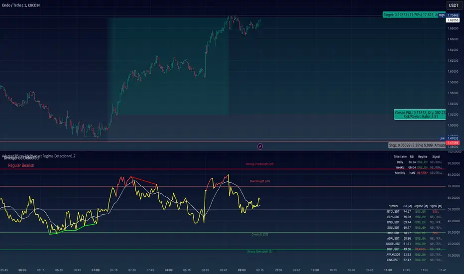
RSI + Normalized Fisher Transform with SignalsThis indicator combines three tools for market analysis: the Relative Strength Index (RSI), the RSI's moving average, and the Fisher Transform. RSI is a momentum oscillator that measures the speed and change of price movements, helping identify overbought and oversold conditions. The RSI moving average is a smoothed version of the RSI that filters noise and confirms trends. The Fisher Transform is a mathematical technique that transforms price data into a Gaussian normal distribution, making it easier to identify turning points. It has been normalized to the same scale as the RSI (0-100) for consistency.
Purpose
The goal of this indicator is to identify potential buy and sell opportunities with varying degrees of strength (strong and weak). By combining the RSI, its moving average, and the Fisher Transform, the indicator ensures signals are based on both momentum and reversals, making it highly versatile across different market conditions.
Key Features
This indicator provides strong and weak buy and sell signals. A strong buy occurs when the RSI crosses above its moving average while both the RSI and its moving average are oversold (below the default threshold of 30), and the Fisher Transform reverses direction within the same or prior bar while also being oversold. A weak buy occurs when the Fisher Transform is oversold, and the RSI crosses above its moving average while its value is between the default oversold threshold (30) and 50. A strong sell occurs when the RSI crosses below its moving average while both the RSI and its moving average are overbought (above the default threshold of 70), and the Fisher Transform reverses direction within the same or prior bar while also being overbought. A weak sell occurs when the Fisher Transform is overbought, and the RSI crosses below its moving average while its value is between 50 and the default overbought threshold (70).
The indicator includes customizable thresholds and lengths. Users can adjust the oversold and overbought thresholds to suit their trading style. The RSI length, moving average length, and Fisher Transform length are also customizable. The Fisher Transform is scaled to the RSI’s range of 0-100 to simplify analysis and signal interpretation.
How to Use the Indicator
On the chart, you will see the RSI line in blue, the RSI moving average in orange, and the Fisher Transform in purple. Horizontal lines at the default oversold (30) and overbought (70) levels mark critical zones for signals. Adjust these thresholds in the indicator settings as needed.
Strong buy signals are shown as larger, darker green arrows below the price. Weak buy signals are small lime arrows below the price. Strong sell signals are larger, darker red arrows above the price. Weak sell signals are small fuchsia arrows above the price.
Signal Interpretation
A strong buy indicates a highly favorable buying opportunity. This typically occurs when the asset is in a downtrend but shows signs of reversal, particularly in oversold zones. A weak buy suggests a potential buying opportunity but with less conviction, often when the market is neutral to slightly bearish but showing upward momentum. A strong sell indicates a highly favorable selling opportunity, usually occurring when the asset is in an uptrend but shows signs of reversal, particularly in overbought zones. A weak sell suggests a potential selling opportunity but with less conviction, often in neutral to slightly bullish markets showing downward momentum.
Practical Tips
Avoid using signals in isolation. Combine this indicator with other tools such as trendlines, moving averages, or support/resistance levels for greater accuracy. Adjust the parameters for different assets to match their volatility. For volatile assets, consider wider thresholds like 20/80 for oversold/overbought levels. For less volatile assets, tighter thresholds like 35/65 may be more appropriate. Use higher timeframes to confirm signals before trading on lower timeframes. Be cautious in sideways markets, as both RSI and the Fisher Transform perform better in trending conditions.
Instructions for Adjustments
To change the oversold or overbought levels, open the indicator settings by clicking the gear icon and modify the "Oversold Threshold" and "Overbought Threshold" values. To adjust lengths for RSI and Fisher Transform, update the "RSI Length," "RSI Moving Average Length," and "Fisher Transform Length" settings. If needed, toggle signal visibility by enabling or disabling specific arrows (Strong Buy, Weak Buy, Strong Sell, Weak Sell) in the "Style" tab.
Best Practices
Risk management is essential. Always set appropriate stop-loss levels and position sizes based on your risk tolerance. Backtest the indicator on historical data to understand its performance and behavior for your chosen asset and timeframe. Combining this indicator with volume or volatility analysis (Bollinger Band Width, for example) can help confirm signal validity.
This indicator simplifies decision-making by identifying high-probability trading opportunities using a combination of momentum, trend, and reversals. Follow these instructions to fully utilize its capabilities without needing to analyze the underlying code.
ADX Breakout Strategy█ OVERVIEW
The ADX Breakout strategy leverages the Average Directional Index (ADX) to identify and execute breakout trades within specified trading sessions. Designed for the NQ and ES 30-minute charts, this strategy aims to capture significant price movements while managing risk through predefined stop losses and trade limits.
This strategy was taken from a strategy that was posted on YouTube. I would link the video, but I believe is is "against house rules".
█ CONCEPTS
The strategy is built upon the following key concepts:
ADX Indicator: Utilizes the ADX to gauge the strength of a trend. Trades are initiated when the ADX value is below a certain threshold, indicating potential for trend development.
Trade Session Management: Limits trading to specific hours to align with optimal market activity periods.
Risk Management: Implements a fixed dollar stop loss and restricts the number of trades per session to control exposure.
█ FEATURES
Customizable Stop Loss: Set your preferred stop loss amount to manage risk effectively.
Trade Session Configuration: Define the trading hours to focus on the most active market periods.
Entry Conditions: Enter long positions when the price breaks above the highest close in the lookback window and the ADX indicates potential trend strength.
Trade Limits: Restrict the number of trades per session to maintain disciplined trading.
Automated Exit: Automatically closes all positions at the end of the trading session to avoid overnight risk.
█ HOW TO USE
Configure Inputs :
Stop Loss ($): Set the maximum loss per trade.
Trade Session: Define the active trading hours.
Highest Lookback Window: Specify the number of bars to consider for the highest close.
Apply the Strategy :
Add the ADX Breakout strategy to your chart on TradingView.
Ensure you are using a 30-minute timeframe for optimal performance.
█ LIMITATIONS
Market Conditions: The strategy is optimized for trending markets and may underperform in sideways or highly volatile conditions.
Timeframe Specific: Designed specifically for 30-minute charts; performance may vary on different timeframes.
Single Asset Focus: Primarily tested on NQ and ES instruments; effectiveness on other symbols is not guaranteed.
█ DISCLAIMER
This ADX Breakout strategy is provided for educational and informational purposes only. It is not financial advice and should not be construed as such. Trading involves significant risk, and you may incur substantial losses. Always perform your own analysis and consider your financial situation before using this or any other trading strategy. The source material for this strategy is publicly available in the comments at the beginning of the code script. This strategy has been published openly for anyone to review and verify its methodology and performance.

Global Index Spread RSI StrategyThis strategy leverages the relative strength index (RSI) to monitor the price spread between a global benchmark index (such as AMEX) and the currently opened asset in the chart window. By calculating the spread between these two, the strategy uses RSI to identify oversold and overbought conditions to trigger buy and sell signals.
Key Components:
Global Benchmark Index: The strategy compares the current asset with a predefined global index (e.g., AMEX) to measure relative performance. The choice of a global benchmark allows the trader to analyze the current asset's movement in the context of broader market trends.
Spread Calculation:
The spread is calculated as the percentage difference between the current asset's closing price and the global benchmark index's closing price:
Spread=Current Asset Close−Global Index CloseGlobal Index Close×100
Spread=Global Index CloseCurrent Asset Close−Global Index Close×100
This metric provides a measure of how the current asset is performing relative to the global index. A positive spread indicates the asset is outperforming the benchmark, while a negative spread signals underperformance.
RSI of the Spread: The RSI is then calculated on the spread values. The RSI is a momentum oscillator that ranges from 0 to 100 and is commonly used to identify overbought or oversold conditions in asset prices. An RSI below 30 is considered oversold, indicating a potential buying opportunity, while an RSI above 70 is overbought, suggesting that the asset may be due for a pullback.
Strategy Logic:
Entry Condition: The strategy enters a long position when the RSI of the spread falls below the oversold threshold (default 30). This suggests that the asset may have been oversold relative to the global benchmark and might be due for a reversal.
Exit Condition: The strategy exits the long position when the RSI of the spread rises above the overbought threshold (default 70), indicating that the asset may have become overbought and a price correction is likely.
Visual Reference:
The RSI of the spread is plotted on the chart for visual reference, making it easier for traders to monitor the relative strength of the asset in relation to the global benchmark.
Overbought and oversold levels are also drawn as horizontal reference lines (70 and 30), along with a neutral level at 50 to show market equilibrium.
Theoretical Basis:
The strategy is built on the mean reversion principle, which suggests that asset prices tend to revert to a long-term average over time. When prices move too far from this mean—either being overbought or oversold—they are likely to correct back toward equilibrium. By using RSI to identify these extremes, the strategy aims to profit from price reversals.
Mean Reversion: According to financial theory, asset prices oscillate around a long-term average, and any extreme deviation (overbought or oversold conditions) presents opportunities for price corrections (Poterba & Summers, 1988).
Momentum Indicators (RSI): The RSI is widely used in technical analysis to measure the momentum of an asset. Its application to the spread between the asset and a global benchmark allows for a more nuanced view of relative performance and potential turning points in the asset's price trajectory.
Practical Application:
This strategy works best in markets where relative strength is a key factor in decision-making, such as in equity indices, commodities, or forex markets. By assessing the performance of the asset relative to a global benchmark and utilizing RSI to identify extremes in price movements, the strategy helps traders to make more informed decisions based on potential mean reversion points.
While the "Global Index Spread RSI Strategy" offers a method for identifying potential price reversals based on relative strength and oversold/overbought conditions, it is important to recognize that no strategy is foolproof. The strategy assumes that the historical relationship between the asset and the global benchmark will hold in the future, but financial markets are subject to a wide array of unpredictable factors that can lead to sudden changes in price behavior.
Risk of False Signals:
The strategy relies heavily on the RSI to trigger buy and sell signals. However, like any momentum-based indicator, RSI can generate false signals, particularly in highly volatile or trending markets. In such conditions, the strategy may enter positions too early or exit too late, leading to potential losses.
Market Context:
The strategy may not account for macroeconomic events, news, or other market forces that could cause sudden shifts in asset prices. External factors, such as geopolitical developments, monetary policy changes, or financial crises, can cause a divergence between the asset and the global benchmark, leading to incorrect conclusions from the strategy.
Overfitting Risk:
As with any strategy that uses historical data to make decisions, there is a risk of overfitting the model to past performance. This could result in a strategy that works well on historical data but performs poorly in live trading conditions due to changes in market dynamics.
Execution Risks:
The strategy does not account for slippage, transaction costs, or liquidity issues, which can impact the execution of trades in real-market conditions. In fast-moving markets, prices may move significantly between order placement and execution, leading to worse-than-expected entry or exit prices.
No Guarantee of Profit:
Past performance is not necessarily indicative of future results. The strategy should be used with caution, and risk management techniques (such as stop losses and position sizing) should always be implemented to protect against significant losses.
Traders should thoroughly test and adapt the strategy in a simulated environment before applying it to live trades, and consider seeking professional advice to ensure that their trading activities align with their risk tolerance and financial goals.
References:
Poterba, J. M., & Summers, L. H. (1988). Mean Reversion in Stock Prices: Evidence and Implications. Journal of Financial Economics, 22(1), 27-59.

Multi-Symbol Scanner: Advanced EMA-RSI-Volume Strategy# Multi-Symbol Tech Stock Scanner: Advanced EMA-RSI-Volume Strategy
## Technical Analysis Methodology
This scanner implements a sophisticated multi-timeframe analysis approach combining three key technical elements:
### 1. Dual EMA System (Primary Trend Detection)
- **Long-term EMA (820 periods)**: Acts as the primary trend identifier
- Chosen specifically for tech stocks' longer-term price waves
- Helps filter out minor market noise while capturing major trend changes
- 820 periods approximately represents 3.2 years of trading days
- **Medium-term EMA (320 periods)**: Serves as trend confirmation
- Approximately 1.25 years of trading data
- Provides earlier entry signals while maintaining trend reliability
- Helps identify potential trend reversals before the major trend shift
### 2. Volume Analysis Component
The script employs a dynamic volume analysis system:
- Calculates 20-period moving average of volume as baseline
- Requires 1.5x surge above baseline for signal confirmation
- Volume surge requirement helps filter out weak moves and potential false breakouts
- Different from standard volume indicators as it uses adaptive thresholds
### 3. RSI Momentum Filter
Implements a specialized RSI configuration:
- 14-period RSI with dynamic overbought/oversold levels
- Oversold threshold: 30 (customizable)
- Overbought threshold: 70 (customizable)
- Used as a confirmation tool rather than primary signal generator
## Signal Generation Logic
### Buy Signal Requirements
1. Price must cross above 820 EMA (PRIMARY CONDITION)
2. Current price must be above 320 EMA (CONFIRMATION)
3. RSI must be above 30 but below 70 (MOMENTUM CHECK)
4. Volume must be 1.5x above 20-period average (STRENGTH VALIDATION)
### Sell Signal Requirements
1. Price must cross below 820 EMA (PRIMARY CONDITION)
2. Current price must be below 320 EMA (CONFIRMATION)
3. RSI must be above 30 but below 70 (MOMENTUM CHECK)
4. Volume must be 1.5x above 20-period average (STRENGTH VALIDATION)
## Risk Management Integration
The script automatically calculates key risk levels based on volatility:
1. **Stop Loss Calculation**:
- Default: 2% below entry for buys
- Dynamically adjusted based on price point
- Can be modified through input parameters
2. **Take Profit Targets**:
- Primary target: 6% above entry (3:1 reward-risk ratio)
- Based on historical tech stock movement patterns
- Adjustable through input parameters
## Multi-Symbol Implementation
The scanner monitors 6 symbols simultaneously using:
- Separate security calls for each data point
- Optimized data requests to prevent overload
- Individual signal processing for each symbol
- Synchronized alert generation system
## Technical Implementation Details
1. **Data Processing**:
```
- Security data requests on 10-minute timeframe
- Individual EMA calculations per symbol
- Separate volume analysis threads
- RSI calculations with standard deviation normalization
```
2. **Signal Processing**:
```
- Cross-verification of all conditions
- Time-based signal validation
- Volume surge confirmation
- Trend alignment check
```
3. **Alert System**:
```
- Bar-close confirmation required
- Multi-condition validation
- Detailed price level inclusion
- Risk parameter integration
```
## Optimization Features
1. **Memory Usage**:
- Optimized security calls
- Efficient data structure
- Reduced redundant calculations
2. **Processing Efficiency**:
- Single-pass data analysis
- Combined indicator calculations
- Streamlined alert generation
## Practical Application
The system is designed for:
1. Swing Trading (primary use)
2. Position Trading (secondary use)
3. Technical Breakout Trading
Optimal timeframes:
- Primary: 4H charts
- Secondary: Daily charts
- Verification: 1H charts
## Default Configuration
The scanner is preset to monitor key tech stocks:
- TSLA: High-volatility tech leader
- NVDA: Semiconductor sector benchmark
- AVGO: Stable tech infrastructure
- TSM: Global chip manufacturer
- META: Social media sector leader
- AMZN: E-commerce/Cloud computing leader
Each symbol can be modified through input parameters.
## Version Information
- Current Version: 1.3
- Last Updated: November 2024
- Compatibility: TradingView Pro/Pro+/Premium
## Limitations & Considerations
- Limited to 6 symbols due to TradingView security request limits
- Requires consistent market volume for optimal performance
- Best suited for liquid stocks with significant daily volume
- May need parameter adjustments during extreme market conditions

SW Gann Pressure time from tops and bottomsW.D. Gann's trading techniques often emphasized the significance of time in the markets, believing that specific time intervals could influence price movements. Here’s how the 30, 60, 90, 120, 180, and 270 bar intervals relate to Gann's rules:
1. **30 Bars**:
- Gann often viewed shorter time frames as critical for identifying short-term trends. A 30-bar interval can signify minor cycles or potential turning points in price.
2. **60 Bars**:
- This interval is significant as Gann believed in the importance of quarterly cycles. A 60-bar mark could indicate a completion of a two-month cycle, often leading to retracements or reversals.
3. **90 Bars**:
- Gann considered 90 days (or bars) to represent a quarter. This interval can signify a substantial shift in market sentiment or a pivotal point in a longer trend.
4. **120 Bars**:
- The 120-bar mark corresponds to about four months. Gann viewed longer intervals as more significant, often leading to major shifts in market trends.
5. **180 Bars**:
- A 180-bar period relates to a semi-annual cycle, which Gann regarded as critical for major support and resistance levels. Price action around this interval can reveal potential long-term trend reversals.
6. **270 Bars**:
- Gann believed that longer cycles, such as 270 bars (approximately nine months), could indicate significant market phases. This interval may represent major turning points and help identify long-term trends.
### Application in Trading:
- **Identifying Trends**: Traders can use these intervals to spot potential trend reversals or continuations based on Gann’s principles of market cycles.
- **Setting Targets and Stops**: Knowing where these key bars fall can help in setting profit targets and stop-loss orders.
- **Analyzing Market Sentiment**: Price reactions at these intervals can provide insights into market psychology and sentiment shifts.
By marking these intervals on a chart, traders can visually assess when price action aligns with Gann's theories, helping them make more informed trading decisions based on historical patterns and cycles.
30D Vs 90D Historical VolatilityVolatility equals risk for an underlying asset's price meaning bullish volatility is bearish for prices while bearish volatility is bullish. This compares 30-Day Historical Volatility to 90-Day Historical Volatility.
When the 30-Day crosses under the 90-day, this is typically when asset prices enter a bullish trend.
Conversely, When the 30-Day crosses above the 90-Day, this is when asset prices enter a bearish trend.
Peaks in volatility are bullish divergences while troughs are bearish divergences.
