SPX +10 / -10 From 9:30 Open//@version=5
indicator("SPX +10 / -10 From 9:30 Open", overlay=true)
// Exchange Time (New York)
sess = input.session("0930-1600", "Regular Session (ET)")
// Detect session and 9:30 AM bar
inSession = time(timeframe.period, sess)
// Capture the 9:30 AM open
var float open930 = na
if inSession
// If this is the first bar of the session (9:30 AM)
if time(timeframe.period, sess) == na
open930 := open
else
open930 := na
// Calculate movement from 9:30 AM open
up10 = close >= open930 + 10
dn10 = close <= open930 - 10
// Plot reference lines
plot(open930, "9:30 AM Open", color=color.orange)
plot(open930 + 10, "+10 Level", color=color.green)
plot(open930 - 10, "-10 Level", color=color.red)
// Alert conditions
alertcondition(up10, title="SPX Up +10", message="SPX moved UP +10 from the 9:30 AM open")
alertcondition(dn10, title="SPX Down -10", message="SPX moved DOWN -10 from the 9:30 AM open")
// Plot signals on chart
plotshape(up10, title="+10 Hit", style=shape.labelup, color=color.green, text="+10", location=location.belowbar, size=size.tiny)
plotshape(dn10, title="-10 Hit", style=shape.labeldown, color=color.red, text="-10", location=location.abovebar, size=size.tiny)
Search in scripts for "创业板etf"

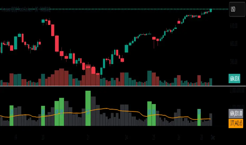
Unusual Volume//@version=5
indicator("Unusual Volume", overlay=false)
// --- Inputs ---
len = input.int(20, "Average Volume Length", minval=1)
mult = input.float(2.0, "Unusual Volume Multiplier", step=0.1)
// --- Calculations ---
avgVol = ta.sma(volume, len)
ratio = volume / avgVol
isBigVol = ratio > mult
// --- Plots ---
plot(volume, "Volume", style=plot.style_columns,
color = isBigVol ? color.new(color.green, 0) : color.new(color.gray, 60))
plot(avgVol, "Average Volume", color=color.orange)
// Mark unusual volume bars
plotshape(isBigVol, title="Unusual Volume Marker",
location=location.bottom, style=shape.triangleup,
color=color.green, size=size.tiny, text="UV")
// Optional: show ratio in Data Window
var label ratioLabel = na

Daily % Change TableDaily % Change Table — Indicator Summary
This indicator provides a compact performance summary for daily candles, designed for backtesting and daily-session analysis. It displays a table in the top-right corner of the chart showing three key percentage-change statistics based on the current candle:
1. Prior Change
Percentage move from the close two days ago to the prior day’s close.
Useful for understanding momentum and context heading into the current session.
2. Change
Percentage move from the prior day's close to the current candle’s close.
Shows today’s full-session change.
3. Premarket
Percentage move from the prior day's close to the current day’s open.
Helps quantify overnight sentiment and gap activity.
Features
Clean, unobtrusive table display
Automatically updates on the most recent bar
Designed for use on Daily timeframe
Useful for gap analysis, backtesting, and volatility/momentum studies

Unusual Volume//@version=5
indicator("Unusual Volume", overlay=false)
// --- Inputs ---
len = input.int(20, "Average Volume Length", minval=1)
mult = input.float(2.0, "Unusual Volume Multiplier", step=0.1)
// --- Calculations ---
avgVol = ta.sma(volume, len)
ratio = volume / avgVol
isBigVol = ratio > mult
// --- Plots ---
plot(volume, "Volume", style=plot.style_columns,
color = isBigVol ? color.new(color.green, 0) : color.new(color.gray, 60))
plot(avgVol, "Average Volume", color=color.orange)
// Mark unusual volume bars
plotshape(isBigVol, title="Unusual Volume Marker",
location=location.bottom, style=shape.triangleup,
color=color.green, size=size.tiny, text="UV")
// Optional: show ratio in Data Window
var label ratioLabel = na
Future High LinePlot a horizontal line from the current high n bars into the future. Line is user configurable.
Works well with Ichimoku Cloud. When line (26 bars) rises into an overhead cloud, this often signals bullish price movement.

10/20 EMA 50/100/200 SMA — by mijoomoCreated by mijoomo.
This indicator combines EMA 10 & EMA 20 with SMA 50/100/200 in one clean package.
Each moving average is toggleable, fully labeled, and alert-compatible.
Designed for traders who want a simple and effective multi-MA trend tool.

Gold Master: Swing + Daily Scalp (Fixed & Working)How to use it correctly
Daily chart → Focus only on big green/red triangles (Swing trades)
5m / 15m / 1H chart → Focus on small circles (Scalp trades)
You can turn each system on/off independently in the settings
Works perfectly on XAUUSD, GLD, GC futures, and even DXY (inverse signals).

Gamma Levels w/AlertsPlots Gamma Levels for identifying Market Positioning. Has alert function on the specific levels.
---To apply to different tickers You Must:
1. apply to chart layout
2. input ticker specific levels
3. Save as an INDICATOR TEMPLATE titled same as ticker (check the remember symbol box)
Now when switching to different tickers, simply open that template

Advanced Trading System - Volume Profile + BB + RSI + FVG + FibAdvanced Multi-Indicator Trading System with Volume Profile, Bollinger Bands, RSI, FVG & Fibonacci
Overview
This comprehensive trading indicator combines five powerful technical analysis tools into one unified system, designed to identify high-probability trading opportunities with precision entry and exit signals. The indicator integrates Volume Profile analysis, Bollinger Bands, RSI momentum, Fair Value Gaps (FVG), and Fibonacci retracement levels to provide traders with a complete market analysis framework.
Key Features
1. Volume Profile & Point of Control (POC)
Automatically calculates the Point of Control - the price level with the highest trading volume
Identifies Value Area High (VAH) and Value Area Low (VAL)
Updates dynamically based on customizable lookback periods
Helps identify key support and resistance zones where institutional traders are active
2. Bollinger Bands Integration
Standard 20-period Bollinger Bands with customizable multiplier
Identifies overbought and oversold conditions
Measures market volatility through band width
Signals generated when price approaches extreme levels
3. RSI Momentum Analysis
14-period Relative Strength Index with visual background coloring
Overbought (70) and oversold (30) threshold alerts
Integrated into buy/sell signal logic for confirmation
Real-time momentum tracking in info dashboard
4. Fair Value Gap (FVG) Detection
Automatically identifies bullish and bearish fair value gaps
Visual representation with colored boxes
Highlights imbalance zones where price may return
Used for high-probability entry confirmation
5. Fibonacci Retracement Levels
Auto-calculated based on recent swing high/low
Key levels: 23.6%, 38.2%, 50%, 61.8%, 78.6%
Perfect for identifying profit-taking zones
Dynamic lines that update with market movement
6. Smart Signal Generation
The indicator generates BUY and SELL signals based on multi-condition confluence:
BUY Signal Requirements:
Price near lower Bollinger Band
RSI in oversold territory (< 30)
High volume confirmation (optional)
Bullish FVG or POC alignment
SELL Signal Requirements:
Price near upper Bollinger Band
RSI in overbought territory (> 70)
High volume confirmation (optional)
Bearish FVG or POC alignment
7. Automated Take Profit Levels
Three dynamic profit targets: 1%, 2%, and 3%
Automatically calculated from entry price
Visual markers on chart
Individual alerts for each level
8. Comprehensive Alert System
The indicator includes 10+ alert types:
Buy signal alerts
Sell signal alerts
Take profit level alerts (TP1, TP2, TP3)
Fibonacci level cross alerts
RSI overbought/oversold alerts
Bullish/Bearish FVG detection alerts
9. Real-Time Info Dashboard
Live display of all key metrics
Color-coded for quick visual analysis
Shows RSI, BB Width, Volume ratio, POC, Fib levels
Current signal status (BUY/SELL/WAIT)
How to Use
Setup
Add the indicator to your chart
Adjust parameters based on your trading style and timeframe
Set up alerts by clicking "Create Alert" and selecting desired conditions
Recommended Timeframes
Scalping: 5m - 15m
Day Trading: 15m - 1H
Swing Trading: 4H - Daily
Parameter Customization
Volume Profile Settings:
Length: 100 (adjust for more/less historical data)
Rows: 24 (granularity of volume distribution)
Bollinger Bands:
Length: 20 (standard period)
Multiplier: 2.0 (adjust for tighter/wider bands)
RSI Settings:
Length: 14 (standard momentum period)
Overbought: 70
Oversold: 30
Fibonacci:
Lookback: 50 (swing high/low detection period)
Signal Settings:
Volume Filter: Enable/disable volume confirmation
Volume MA Length: 20 (for volume comparison)
Trading Strategy Examples
Strategy 1: Trend Reversal
Wait for BUY signal at lower Bollinger Band
Confirm with bullish FVG or POC support
Enter position
Take partial profits at Fib 38.2% and 50%
Exit remaining position at TP3 or SELL signal
Strategy 2: Breakout Confirmation
Monitor price approaching POC level
Wait for volume spike
Enter on signal confirmation with FVG alignment
Use Fibonacci levels for scaling out
Strategy 3: Range Trading
Identify POC as range midpoint
Buy at lower BB with oversold RSI
Sell at upper BB with overbought RSI
Use FVG zones for additional confirmation
Best Practices
✅ Do:
Use multiple timeframe analysis
Combine with price action analysis
Set stop losses below/above recent swing points
Scale out at Fibonacci levels
Wait for volume confirmation on signals
❌ Don't:
Trade every signal blindly
Ignore overall market context
Use on extremely low timeframes without testing
Neglect risk management
Trade during low liquidity periods
Risk Management
Always use stop losses
Risk no more than 1-2% per trade
Consider market conditions and volatility
Scale position sizes based on signal strength
Use the volume filter for additional confirmation
Technical Specifications
Pine Script Version: 6
Overlay: Yes (displays on main chart)
Max Boxes: 500 (for FVG visualization)
Max Lines: 500 (for Fibonacci levels)
Alerts: 10+ customizable conditions
Performance Notes
This indicator works best in:
Trending markets with clear momentum
High-volume trading sessions
Assets with good liquidity
When multiple signals align
Less effective in:
Extremely choppy/sideways markets
Low-volume periods
During major news events (high volatility)
Updates & Support
This indicator is actively maintained and updated. Future enhancements may include:
Additional volume profile features
More sophisticated FVG tracking
Enhanced alert customization
Backtesting integration
Disclaimer
This indicator is for educational and informational purposes only. It does not constitute financial advice. Past performance does not guarantee future results. Always conduct your own research and consider consulting with a financial advisor before making trading decisions. Trading involves substantial risk of loss.

5m1m RSI StrategyIdentify 15m RSI divergence as identified by 5m RSI confirmation. Exit on 1m correction.

Yit's Risk CalculatorIntroducing a risk a bulletproof risk calculator.
I'm tired of sitting on my brokerage, messing with my shares to buy while price action leaves me in the dust.
For my breakout strategy execution is everything i dont have time to stop and think.
within the Indicator settings you have free reign to change account size and risk%
*the stop loss is glued to the low of the day*

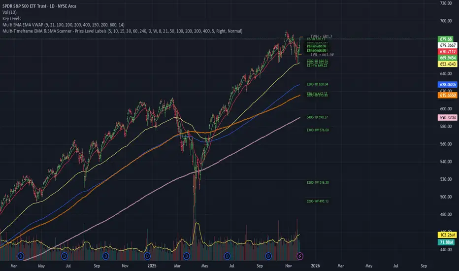
Multi-Timeframe EMA & SMA Scanner - Price Level LabelsOverview
A powerful multi-timeframe moving average scanner that displays EMA and SMA levels from up to 8 different timeframes simultaneously on your chart. Perfect for identifying key support/resistance levels, confluence zones, and multi-timeframe trend analysis.
Key Features
📊 Multi-Timeframe Analysis
Monitor up to 8 different timeframes simultaneously (5m, 10m, 15m, 30m, 1H, 4H, 1D, 1W)
Each timeframe can be independently enabled/disabled
Fully customizable timeframe selection
📈 Comprehensive Moving Averages
5 configurable EMA periods (default: 8, 21, 50, 100, 200)
2 configurable SMA periods (default: 200, 400)
All periods are fully customizable to match your trading strategy
🎯 Smart Price Level Labels
Labels positioned at actual price levels (not in a list)
Color-coded labels for easy identification
Dynamic text color: Green when price is above, Red when below
Compact notation: E8-5m means EMA 8 on 5-minute timeframe
Adjustable label offset from current price
📉 Optional Horizontal Lines
Dotted reference lines at each MA level
Color-matched to corresponding MA type
Can be toggled on/off independently
📋 Comprehensive Data Table
Shows all MA values organized by timeframe
Displays percentage distance from current price
Trend indicator (Strong Up/Up/Neutral/Down/Strong Down)
EMA alignment status (Bullish/Bearish/Mixed)
Color-coded cells for quick visual analysis
🎨 Full Customization
Individual color settings for each MA type
Adjustable table size (Tiny/Small/Normal/Large)
Choose table position (Left/Right)
Toggle any MA or timeframe on/off
🔔 Built-in Alerts
Golden Cross detection (EMA 50 crosses above EMA 200)
Death Cross detection (EMA 50 crosses below EMA 200)
Price crossing major EMAs
Available for multiple timeframes
How to Use
For Day Traders:
Enable lower timeframes (5m, 10m, 15m, 30m)
Focus on faster EMAs (8, 21, 50)
Watch for confluence zones where multiple timeframe MAs cluster
For Swing Traders:
Enable higher timeframes (1H, 4H, 1D)
Use all EMAs plus SMAs for broader perspective
Look for alignment across timeframes for high-probability setups
For Position Traders:
Focus on daily and weekly timeframes
Emphasize 100, 200 EMAs and 200, 400 SMAs
Use for long-term trend confirmation
Understanding the Labels
Label Format: E8-5m 45250.50
E8 = EMA with period 8
5m = 5-minute timeframe
45250.50 = Current price level
Green text = Price is currently above this level (potential support)
Red text = Price is currently below this level (potential resistance)
For SMAs: S200-1D 44500.00
S200 = SMA with period 200
1D = Daily timeframe
Trading Applications
Support/Resistance Identification
MAs act as dynamic support and resistance levels
Multiple timeframe MAs create stronger zones
Confluence Trading
When multiple MAs from different timeframes cluster together, it creates high-probability zones
These areas often result in strong reactions
Trend Analysis
Check the Alignment column: Bullish alignment = all EMAs in ascending order
Trend column shows overall price position relative to all MAs
Entry/Exit Timing
Use lower timeframe MAs for precise entries
Use higher timeframe MAs for trend direction and exits
Settings Guide
Timeframes Section:
Select and enable/disable up to 8 timeframes
Default: 5m, 10m, 15m, 30m, 1H, 4H, 1D, 1W
MA Periods Section:
Customize all EMA and SMA periods
Default EMAs: 8, 21, 50, 100, 200
Default SMAs: 200, 400
Display Section:
Toggle price labels and horizontal lines
Adjust label offset (distance from right edge)
Show/hide data table
Choose table position and size
Colors Section:
Customize colors for each MA type
Each MA has independent color control
Pro Tips
✅ Start with default settings and adjust based on your trading style
✅ Disable timeframes/MAs you don't use to reduce chart clutter
✅ Use the data table for quick overview, labels for precise levels
✅ Look for "confluence clusters" where multiple MAs from different timeframes align
✅ Green labels = potential support, Red labels = potential resistance
✅ Set alerts on key crossovers for automated notifications
Technical Specifications
Pine Script v6
Overlay indicator (displays on main chart)
Maximum 500 labels supported
Real-time updates on each bar close
Compatible with all instruments and timeframes
Perfect For:
Day traders seeking multi-timeframe confirmation
Swing traders looking for high-probability setups
Position traders monitoring long-term trends
Anyone using moving averages as part of their strategy
Note: This indicator does not provide buy/sell signals. It's a tool for analysis and should be used in conjunction with your trading strategy and risk management rules.
Key Levels by Romulus V2This is the updated key levels script I added dynamic levels that change throughout the day opening range high and low and customizable settings to adjust.

Fair Value Gaps (FVG)This indicator automatically detects Fair Value Gaps (FVGs) using the classic 3-candle structure (ICT-style).
It is designed for traders who want clean charts and relevant FVGs only, without the usual clutter from past sessions or tiny, meaningless gaps.
Key Features
• Bullish & Bearish FVG detection
Identifies imbalances where price fails to trade efficiently between candles.
• Automatic FVG removal when filled
As soon as price trades back into the gap, the box is deleted in real time – no more outdated zones on the chart.
• Only shows FVGs from the current session
At the start of each new session, all previous FVGs are cleared.
Perfect for intraday traders who only care about today’s liquidity map.
• Flexible minimum gap size filter
Avoid noise by filtering FVGs using one of three modes:
Ticks (based on market tick size)
Percent (relative to current price)
Points (absolute price distance)
• Right-extension option
Keep gaps extended forward in time or limit them to the candles that created them.
Why This Indicator?
Many FVG indicators overwhelm the chart with zones from previous days or tiny imbalances that don’t matter.
This version keeps things clean, meaningful, and real-time accurate, ideal for day traders who rely on market structure and liquidity.

Daily Gap Highlighter (Partial Gaps + Age Filter)Daily Gap Highlighter – 部分的な窓の未埋めエリアを自動描画
このインジケーターは、日足チャートにおける窓(ギャップ)を自動で検出し、
その後の値動きで一部だけ埋まった場合も、埋め残し部分だけを正確に描画するツールです。
🔍 主な特徴
日足ベースで窓を検出
上窓:当日の安値 > 前日の高値
下窓:当日の高値 < 前日の安値
部分的な窓埋めにも対応
例:窓の90%が埋まった → 残り10%だけ窓として残す
完全に埋まった窓は自動的に削除
窓の“鮮度フィルター”を搭載
指定した日数(デフォルト90日)を経過した古い窓は自動で非表示にできます。
トレンド転換ポイントの可視化に最適
未埋めギャップは多くのトレーダーが注目する価格帯であり、
サポート/レジスタンスとして高い機能を持ちます。
📈 活用例
スイングトレードでのターゲット設定
窓埋めの完了・未完了の判定
重要水平ラインとしての分析
長期的な価格メモリーの可視化
日足チャートを使うトレーダーの方にとって、
“本当に意味のある未埋め窓だけ”が残る実用的なインジケーターです。
🇺🇸 English Description (for TradingView Community)
Daily Gap Highlighter – Precise Partial Gap Visualization
This indicator automatically detects daily price gaps and visualizes them on the chart —
but with one powerful upgrade:
It keeps only the unfilled portion of the gap.
🔍 Key Features
Daily-based gap detection
Up Gap: Today’s Low > Previous High
Down Gap: Today’s High < Previous Low
Partial gap filling supported
Example: If 90% of the gap has been filled,
→ Only the remaining 10% is still shown as an active gap.
Fully filled gaps are automatically removed
Gap “age filter” included
Automatically hide gaps older than a chosen number of days (default: 90).
Great for identifying key market levels
Unfilled gaps often act as strong support/resistance zones
and are widely watched by professional traders.
📈 Use Cases
Setting targets for swing trades
Determining whether a gap is filled or partially filled
Highlighting significant horizontal price levels
Visualizing long-term market memory zones
This tool is ideal for traders who want
a clean and accurate view of meaningful unfilled gaps only.

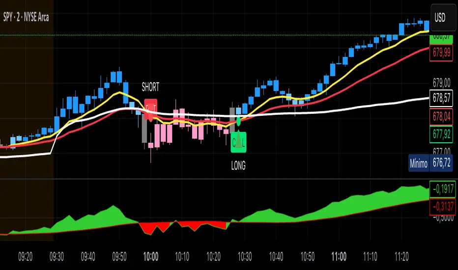
Kai GoNoGo 2mKai GoNoGo 2m is a multi-factor trend confirmation system designed for fast intraday trading on the 2-minute chart.
It combines EMAs, MACD, RSI and ADX through a weighted scoring model to generate clear Go / NoGo conditions for both CALL (long) and PUT (short) setups.
The indicator paints the candles with pure colors to show the current strength of the trend:
Strong Go (Bright Blue): Full bullish alignment across EMAs, momentum and trend strength.
Weak Go (Light Blue): Bullish structure but with softer momentum.
Weak NoGo (Light Pink): Bearish structure starting to develop.
Strong NoGo (Bright Pink): Full bearish alignment across all components.
Neutral (Gray): No trend, compression or transition phase.
Components included:
EMA Trend Structure (9/21/50/100/200)
MACD Momentum (12-26-9)
RSI Confirmation (14)
ADX Trend Strength Filter via DMI (14,14)
Scoring system inspired by the original GoNoGo concept, improved for speed-based trading.
Designed for:
Scalping, 0DTE options, FAST trend continuation entries, and momentum confirmation on QQQ, SPY, NQ, ES and high-beta names.
This version uses pure colors (no gradients) for maximum clarity when trading fast charts.

Key Levels by ROMKey Levels Pro — Long Description
Key Levels Pro is a precision-built market structure indicator designed to instantly identify the most influential price zones driving intraday and swing-level movement. Using adaptive algorithms that track liquidity pockets, volume concentration, volatility shifts, and historical reaction points, the indicator automatically plots dynamic support and resistance levels that institutions consistently respect.
Unlike static horizontal lines or manually drawn zones, Key Levels Pro continuously updates as new order-flow and volatility data comes in. This ensures the indicator reflects the real-time balance of buyers and sellers, not outdated swing points.
The system classifies levels by strength, frequency of reaction, and current market interest. This helps traders instantly see which levels are likely to produce continuation, reversals, or liquidity grabs. High-probability zones are clearly highlighted, allowing you to plan entries, scale-outs, stop placements, and invalidations with confidence.
Whether you trade futures, equities, crypto, or forex, Key Levels Pro becomes the backbone of your strategy. It simplifies complex price action into clean, actionable zones—and makes it easy to anticipate where momentum pauses, accelerates, or completely shifts.

Pivot Reversal Signals - Multi ConfirmationPivot Reversal Signals - Multi-Confirmation System
Overview
A comprehensive reversal detection indicator designed for daytraders that combines six independent technical signals to identify high-probability pivot points. The indicator uses a scoring system to classify signal strength as Weak, Medium, or Strong based on the number of confirmations present.
How It Works
The indicator monitors six key reversal signals simultaneously:
1. RSI Divergence - Detects when price makes new highs/lows but RSI shows weakening momentum
2. MACD Divergence - Identifies divergence between price action and MACD histogram
3. Key Level Touch - Confirms price is at significant support/resistance (previous day high/low, premarket high/low, VWAP, 50 SMA)
4. Reversal Candlestick Patterns - Recognizes bullish/bearish engulfing, hammers, and shooting stars
5. Moving Average Confluence - Validates bounces/rejections at stacked moving averages (9/20/50)
6. Volume Spike - Confirms increased participation (default: 1.5x average volume)
Signal Strength Classification
• Weak (3/6 confirmations) - Small circles for situational awareness only
• Medium (4/6 confirmations) - Regular triangles, viable entry signals
• Strong (5-6/6 confirmations) - Large triangles with background highlight, highest probability setups
Visual Features
• Entry Signals: Green triangles (up) for long entries, red triangles (down) for short entries
• Exit Warnings: Orange X markers when opposing signals appear
• Signal Labels: Show confirmation score (e.g., "5/6") and strength level
• Key Levels Displayed:
o Previous Day High/Low - Solid green/red lines (uses actual daily data)
o Premarket High/Low - Blue/orange circles (4:00 AM - 9:30 AM EST)
o VWAP - Purple line
o Moving Averages - 9 EMA (blue), 20 EMA (orange), 50 SMA (red)
• Background Tinting: Subtle color on strongest reversal zones
Key Level Detection
The indicator uses request.security() to accurately fetch previous day's high/low from daily timeframe data, ensuring precise level placement. Premarket high/low levels are dynamically tracked during premarket sessions (4:00 AM - 9:30 AM EST) and plotted throughout the trading day, providing critical support/resistance zones that often influence price action during regular hours.
Customizable Parameters
• Signal strength thresholds (adjust required confirmations)
• RSI settings (length, overbought/oversold levels)
• MACD parameters (fast/slow/signal lengths)
• Moving average periods
• Volume spike multiplier
• Toggle individual display elements (levels, MAs, labels)
Best Practices
• Use on 5-minute charts for entries, confirm on 15-minute for direction
• Focus on Medium and Strong signals; Weak signals provide context only
• Strong signals (5-6 confirmations) have the highest win rate
• Pay special attention to reversals at premarket high/low - these levels frequently hold
• Previous day high/low often acts as major support/resistance
• Always use proper risk management and stop losses
• Works best in moderately trending markets
Alert Capabilities
Set custom alerts for:
• Strong long/short signals
• All entry signals (medium + strong)
• Exit warnings for open positions
Ideal For
• Daytraders and scalpers (especially SPY, QQQ, and liquid equities)
• Swing traders seeking precise entries
• Traders who prefer confirmation-based systems
• Anyone looking to reduce false signals with multi-factor validation
• Traders who utilize premarket levels in their strategy
Technical Notes
• Uses Pine Script v6
• Premarket hours: 4:00 AM - 9:30 AM EST
• Previous day levels pulled from daily timeframe for accuracy
• Maximum 500 labels to maintain chart performance
• All key levels update dynamically in real-time
________________________________________
Note: This indicator provides signal analysis only and should be used as part of a complete trading strategy. Past performance does not guarantee future results. Always practice proper risk management.

SPY Daily Gamma Levels [Manual Input With Alerts]Overview This indicator plots key options-based support and resistance levels (Gamma Exposure / GEX) directly on your chart. Unlike standard technical analysis, these levels (Call Wall, Gamma Flip, Put Support, and Volatility Trigger) represent where Market Makers are positioned, often acting as "magnets" or "repellents" for price action.
Important Note: TradingView Pine Script cannot currently access external options open interest data natively. Therefore, this is a Manual Input Indicator. You must update the four price levels in the settings each morning before the market opens.
Key Features:
4 Key Levels: Plots the Call Wall, Gamma Flip (Zero Gamma), Put Support, and Volatility Trigger.
Auto-Cleaning: Automatically deletes yesterday's lines to keep your chart clean; lines only show for the current session.
Alerts Included: Built-in alert conditions allow you to set notifications when price crosses the Gamma Flip or breaks the Vol Trigger.
Customization: Fully customizable colors and line styles.
Best Practices:
Timeframe: Works best on 15-minute charts for trend identification and 5-minute charts for entry execution.
Strategy:
Above Gamma Flip: Market generally stabilizes; dealers buy dips.
Below Gamma Flip: Volatility expands; dealers sell rips.
Below Vol Trigger: "Danger Zone" – expect accelerated selling pressure.
How to Get the Data (The AI Workflow)
Since these numbers change daily, I use Google Gemini to fetch the data and remind me every morning. Here is how you can set up the same automated workflow:
1. The Prompt You can ask Gemini (or your preferred AI) the following prompt manually each morning:
"Find the daily SPY Call Wall, Gamma Flip, Put Support, and Vol Trigger levels for today to input into my TradingView indicator."
2. Automating the Routine I have set up a scheduled daily reminder with Gemini. To do this yourself, simply ask Gemini:
"Can you schedule a daily task to search for these SPY Gamma levels and send them to me every morning at 8:00 AM?"
3. Updating the Chart
Receive the notification from the AI.
Open the Indicator Settings in TradingView.
Type in the new numbers.
The chart updates instantly.
Disclaimer: This tool is for educational purposes only. Gamma levels are estimates based on Open Interest and Dealer Gamma exposure models. Always manage your risk.

3x SMA with Fixed TimeframesYou can adjust colors and thickness.
Also can adjust to a fixed timeframe no matter what timeframe you're viewing chart.

8 EMA Candle Color ChangeableJust a quick indicator that I threw together that shows the 8 EMA and changes the candle colors if the candle closes above or below the EMA.

ORB 15min: Break & ConfirmUsing the 15-minute opening candle range, this generates an alert when a 5-minute candle breaks the range and another 5-minute candle closes above the breakout candle's high or the high of any other candle that attempted to break the range.
