Drummond Geometry - Pldot and EnvelopeThis Pine Script will:
1.Calculate and display the PL Dot (Price Level Dot), a moving average that reflects short-term market trends.
2.Plot the Envelope Top and Bottom lines based on averages of previous highs and lows, which represent key areas of resistance and support.
Drummond Geometry Overview
Drummond Geometry is a method of market analysis focused on:
PL Dot : Captures market energy and trend direction. It reacts to price deviations and serves as a magnet for price returns, often referred to as a "PL Dot Refresh."
Envelope Theory : Considers price movements as cycles oscillating between the Envelope Top and Bottom. Prices breaking these boundaries often indicate trends, retracements, or exhaustion.
The geometry helps traders visualize energy flows in the market and anticipate directional changes using established support and resistance zones.
Understanding PL Dot and Envelope Top/Bottom
PL Dot:
Formula: Average(Average(H, L, C) of last three bars)
Usage: Indicates short-term trends:
Trend: PL Dot slopes upward or downward.
Congestion: PL Dot moves horizontally.
Envelope Top and Bottom:
Formula:
Top: (11 H1 + 11 H2 + 11 H3) / 3
Bottom: (11 L1 + 11 L2 + 11 L3) / 3
Usage: Acts as dynamic resistance and support:
Price above the top: Indicates strong bullish momentum.
Price below the bottom: Indicates strong bearish momentum.
Advantages of Drummond Geometry
Clarity of Market Flow: Highlights the relationship between price and key levels (PL Dot, Envelope Top/Bottom).
Predictive Power: Suggests possible reversals or continuation based on energy distribution.
Adaptability: Works across multiple time frames and market types (trending, congestion).
Trading Strategy
PL Dot Trades:
Buy: When price returns to the PL Dot in an uptrend.
Sell: When price returns to the PL Dot in a downtrend.
Envelope Trades:
Reversal: Trade counter to price if it breaks and retreats from the Envelope Top/Bottom.
Continuation: Trade in the direction of price if it sustains movement beyond the Envelope Top/Bottom.
Search in scripts for "电力行业+股票+11年涨幅"

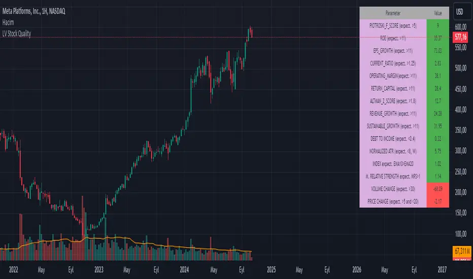
LV Stock QualityCritical financial and technical values are listed in the table.
PIOTROSKI_F_SCORE (expect. >5) -> The Piotroski score is a discrete score between zero and nine that reflects nine criteria used to determine the strength of a firm's financial position. The Piotroski score is used to determine the best value stocks, with nine being the best and zero being the worst. Having a score bigger than 5 is a good sign for the strength of a firm's financial position
ROE (expect. >11) --> Return on equity (ROE) is a measure of a company's financial performance. It is calculated by dividing net income by shareholders' equity. Because shareholders' equity is equal to a company’s assets minus its debt, ROE is a way of showing a company's return on net assets. A “good” ROE will depend on the company’s industry and competitors.
EPS_GROWTH (expect. >11) --> This indicator is calculated as the percentage change in Basic earnings per share for one year. This indicator reflects the growth rate of a company's basic profit per share outstanding for one year. It is calculated based using only common shares. An increase in EPS growth may signal that a company is becoming more profitable and efficient in its operations. A decline in EPS growth may signal that a company is spending more or losing business share. EPS growth should be viewed alongside other metrics like revenue and costs.
CURRENT_RATIO (expect. >1.25) --> The current ratio measures a company’s ability to pay current, or short-term, liabilities (debt and payables) with its current, or short-term, assets (cash, inventory, and receivables). Current ratios over 1.00 indicate that a company's current assets are greater than its current liabilities, meaning it could more easily pay of short-term debts.
OPERATING_MARGIN(expect. >11) --> The operating margin measures how much profit a company makes on a dollar of sales after paying for variable costs of production, such as wages and raw materials, but before paying interest or tax.
RETURN_CAPITAL (expect. >11) --> Return of capital (ROC) is a payment that an investor receives as a portion of their original investment and that is not considered income or capital gains from the investment.
ALTMAN_Z_SCORE (expect. >1.8) --> The Altman Z-score is the output of a credit-strength test that gauges a publicly traded manufacturing company's likelihood of bankruptcy. An Altman Z-score close to 0 suggests a company might be headed for bankruptcy, while a score closer to 3 suggests a company is in solid financial positioning.
REVENUE_GROWTH (expect. >11) --> Quarterly revenue growth is an increase in a company's sales in one quarter compared to sales of a different quarter. Comparing a company's financials from one period to another gives a clear picture of its revenue growth rate and can help investors identify the catalyst for such growth.
SUSTAINABLE_GROWTH (expect. >11) --> The sustainable growth rate (SGR) is the maximum rate of growth that a company or social enterprise can sustain without having to finance growth with additional equity or debt. In other words, it is the rate at which the company can grow while using its own internal revenue without borrowing from outside sources.
DEBT TO INCOME (expect. <0.4) --> A debt-to-income (DTI) ratio is a financial metric used by lenders to determine your borrowing risk. Your DTI ratio represents the total amount of debt you owe compared to the total amount of money you earn each month.
NORMALIZED ATR (expect. <8, W) --> The Normalized Average True Range (Normalized ATR) is an indicator used to measure market volatility by normalizing the average true range values. It does this by dividing the Average True Range (ATR) by the asset's closing price, converting it into a percentage. This normalization allows for the comparison of volatility levels across different securities or market conditions, regardless of the asset's price levels. The Normalized ATR helps traders to adjust their strategies based on relative volatility, rather than absolute price movements.
INDEX expect. EMA10>EMA20 --> it is expected to have EMA 10 > EMA 20 in weekly basis graph. It is known that having a strong trend in index will also increases chance of strong trend on stock levels. You need to select INDEX Market of stock via settings.
M. RELATIVE STRENGTH expect. MRS>1 --> Stan Weinstein uses the Mansfield RS indicator as another relative strength indicator. The indicator measures the variation in the 52-week ratio of stock and market.
VOLUME CHANGE (expect. >30) --> Having an increase on volume comparing to previous week can be a good sign if it occurs at the same time of breakout.
PRICE CHANGE (expect. >5 and <20) --> Having an increase on price comparing to previous week can be a good sign if it occurs at the same time of breakout.
It is better to look on weekly basis graphs.
PubLibTrendLibrary "PubLibTrend"
trend, multi-part trend, double trend and multi-part double trend conditions for indicator and strategy development
rlut()
return line uptrend condition
Returns: bool
dt()
downtrend condition
Returns: bool
ut()
uptrend condition
Returns: bool
rldt()
return line downtrend condition
Returns: bool
dtop()
double top condition
Returns: bool
dbot()
double bottom condition
Returns: bool
rlut_1p()
1-part return line uptrend condition
Returns: bool
rlut_2p()
2-part return line uptrend condition
Returns: bool
rlut_3p()
3-part return line uptrend condition
Returns: bool
rlut_4p()
4-part return line uptrend condition
Returns: bool
rlut_5p()
5-part return line uptrend condition
Returns: bool
rlut_6p()
6-part return line uptrend condition
Returns: bool
rlut_7p()
7-part return line uptrend condition
Returns: bool
rlut_8p()
8-part return line uptrend condition
Returns: bool
rlut_9p()
9-part return line uptrend condition
Returns: bool
rlut_10p()
10-part return line uptrend condition
Returns: bool
rlut_11p()
11-part return line uptrend condition
Returns: bool
rlut_12p()
12-part return line uptrend condition
Returns: bool
rlut_13p()
13-part return line uptrend condition
Returns: bool
rlut_14p()
14-part return line uptrend condition
Returns: bool
rlut_15p()
15-part return line uptrend condition
Returns: bool
rlut_16p()
16-part return line uptrend condition
Returns: bool
rlut_17p()
17-part return line uptrend condition
Returns: bool
rlut_18p()
18-part return line uptrend condition
Returns: bool
rlut_19p()
19-part return line uptrend condition
Returns: bool
rlut_20p()
20-part return line uptrend condition
Returns: bool
rlut_21p()
21-part return line uptrend condition
Returns: bool
rlut_22p()
22-part return line uptrend condition
Returns: bool
rlut_23p()
23-part return line uptrend condition
Returns: bool
rlut_24p()
24-part return line uptrend condition
Returns: bool
rlut_25p()
25-part return line uptrend condition
Returns: bool
rlut_26p()
26-part return line uptrend condition
Returns: bool
rlut_27p()
27-part return line uptrend condition
Returns: bool
rlut_28p()
28-part return line uptrend condition
Returns: bool
rlut_29p()
29-part return line uptrend condition
Returns: bool
rlut_30p()
30-part return line uptrend condition
Returns: bool
dt_1p()
1-part downtrend condition
Returns: bool
dt_2p()
2-part downtrend condition
Returns: bool
dt_3p()
3-part downtrend condition
Returns: bool
dt_4p()
4-part downtrend condition
Returns: bool
dt_5p()
5-part downtrend condition
Returns: bool
dt_6p()
6-part downtrend condition
Returns: bool
dt_7p()
7-part downtrend condition
Returns: bool
dt_8p()
8-part downtrend condition
Returns: bool
dt_9p()
9-part downtrend condition
Returns: bool
dt_10p()
10-part downtrend condition
Returns: bool
dt_11p()
11-part downtrend condition
Returns: bool
dt_12p()
12-part downtrend condition
Returns: bool
dt_13p()
13-part downtrend condition
Returns: bool
dt_14p()
14-part downtrend condition
Returns: bool
dt_15p()
15-part downtrend condition
Returns: bool
dt_16p()
16-part downtrend condition
Returns: bool
dt_17p()
17-part downtrend condition
Returns: bool
dt_18p()
18-part downtrend condition
Returns: bool
dt_19p()
19-part downtrend condition
Returns: bool
dt_20p()
20-part downtrend condition
Returns: bool
dt_21p()
21-part downtrend condition
Returns: bool
dt_22p()
22-part downtrend condition
Returns: bool
dt_23p()
23-part downtrend condition
Returns: bool
dt_24p()
24-part downtrend condition
Returns: bool
dt_25p()
25-part downtrend condition
Returns: bool
dt_26p()
26-part downtrend condition
Returns: bool
dt_27p()
27-part downtrend condition
Returns: bool
dt_28p()
28-part downtrend condition
Returns: bool
dt_29p()
29-part downtrend condition
Returns: bool
dt_30p()
30-part downtrend condition
Returns: bool
ut_1p()
1-part uptrend condition
Returns: bool
ut_2p()
2-part uptrend condition
Returns: bool
ut_3p()
3-part uptrend condition
Returns: bool
ut_4p()
4-part uptrend condition
Returns: bool
ut_5p()
5-part uptrend condition
Returns: bool
ut_6p()
6-part uptrend condition
Returns: bool
ut_7p()
7-part uptrend condition
Returns: bool
ut_8p()
8-part uptrend condition
Returns: bool
ut_9p()
9-part uptrend condition
Returns: bool
ut_10p()
10-part uptrend condition
Returns: bool
ut_11p()
11-part uptrend condition
Returns: bool
ut_12p()
12-part uptrend condition
Returns: bool
ut_13p()
13-part uptrend condition
Returns: bool
ut_14p()
14-part uptrend condition
Returns: bool
ut_15p()
15-part uptrend condition
Returns: bool
ut_16p()
16-part uptrend condition
Returns: bool
ut_17p()
17-part uptrend condition
Returns: bool
ut_18p()
18-part uptrend condition
Returns: bool
ut_19p()
19-part uptrend condition
Returns: bool
ut_20p()
20-part uptrend condition
Returns: bool
ut_21p()
21-part uptrend condition
Returns: bool
ut_22p()
22-part uptrend condition
Returns: bool
ut_23p()
23-part uptrend condition
Returns: bool
ut_24p()
24-part uptrend condition
Returns: bool
ut_25p()
25-part uptrend condition
Returns: bool
ut_26p()
26-part uptrend condition
Returns: bool
ut_27p()
27-part uptrend condition
Returns: bool
ut_28p()
28-part uptrend condition
Returns: bool
ut_29p()
29-part uptrend condition
Returns: bool
ut_30p()
30-part uptrend condition
Returns: bool
rldt_1p()
1-part return line downtrend condition
Returns: bool
rldt_2p()
2-part return line downtrend condition
Returns: bool
rldt_3p()
3-part return line downtrend condition
Returns: bool
rldt_4p()
4-part return line downtrend condition
Returns: bool
rldt_5p()
5-part return line downtrend condition
Returns: bool
rldt_6p()
6-part return line downtrend condition
Returns: bool
rldt_7p()
7-part return line downtrend condition
Returns: bool
rldt_8p()
8-part return line downtrend condition
Returns: bool
rldt_9p()
9-part return line downtrend condition
Returns: bool
rldt_10p()
10-part return line downtrend condition
Returns: bool
rldt_11p()
11-part return line downtrend condition
Returns: bool
rldt_12p()
12-part return line downtrend condition
Returns: bool
rldt_13p()
13-part return line downtrend condition
Returns: bool
rldt_14p()
14-part return line downtrend condition
Returns: bool
rldt_15p()
15-part return line downtrend condition
Returns: bool
rldt_16p()
16-part return line downtrend condition
Returns: bool
rldt_17p()
17-part return line downtrend condition
Returns: bool
rldt_18p()
18-part return line downtrend condition
Returns: bool
rldt_19p()
19-part return line downtrend condition
Returns: bool
rldt_20p()
20-part return line downtrend condition
Returns: bool
rldt_21p()
21-part return line downtrend condition
Returns: bool
rldt_22p()
22-part return line downtrend condition
Returns: bool
rldt_23p()
23-part return line downtrend condition
Returns: bool
rldt_24p()
24-part return line downtrend condition
Returns: bool
rldt_25p()
25-part return line downtrend condition
Returns: bool
rldt_26p()
26-part return line downtrend condition
Returns: bool
rldt_27p()
27-part return line downtrend condition
Returns: bool
rldt_28p()
28-part return line downtrend condition
Returns: bool
rldt_29p()
29-part return line downtrend condition
Returns: bool
rldt_30p()
30-part return line downtrend condition
Returns: bool
dut()
double uptrend condition
Returns: bool
ddt()
double downtrend condition
Returns: bool
dut_1p()
1-part double uptrend condition
Returns: bool
dut_2p()
2-part double uptrend condition
Returns: bool
dut_3p()
3-part double uptrend condition
Returns: bool
dut_4p()
4-part double uptrend condition
Returns: bool
dut_5p()
5-part double uptrend condition
Returns: bool
dut_6p()
6-part double uptrend condition
Returns: bool
dut_7p()
7-part double uptrend condition
Returns: bool
dut_8p()
8-part double uptrend condition
Returns: bool
dut_9p()
9-part double uptrend condition
Returns: bool
dut_10p()
10-part double uptrend condition
Returns: bool
dut_11p()
11-part double uptrend condition
Returns: bool
dut_12p()
12-part double uptrend condition
Returns: bool
dut_13p()
13-part double uptrend condition
Returns: bool
dut_14p()
14-part double uptrend condition
Returns: bool
dut_15p()
15-part double uptrend condition
Returns: bool
dut_16p()
16-part double uptrend condition
Returns: bool
dut_17p()
17-part double uptrend condition
Returns: bool
dut_18p()
18-part double uptrend condition
Returns: bool
dut_19p()
19-part double uptrend condition
Returns: bool
dut_20p()
20-part double uptrend condition
Returns: bool
dut_21p()
21-part double uptrend condition
Returns: bool
dut_22p()
22-part double uptrend condition
Returns: bool
dut_23p()
23-part double uptrend condition
Returns: bool
dut_24p()
24-part double uptrend condition
Returns: bool
dut_25p()
25-part double uptrend condition
Returns: bool
dut_26p()
26-part double uptrend condition
Returns: bool
dut_27p()
27-part double uptrend condition
Returns: bool
dut_28p()
28-part double uptrend condition
Returns: bool
dut_29p()
29-part double uptrend condition
Returns: bool
dut_30p()
30-part double uptrend condition
Returns: bool
ddt_1p()
1-part double downtrend condition
Returns: bool
ddt_2p()
2-part double downtrend condition
Returns: bool
ddt_3p()
3-part double downtrend condition
Returns: bool
ddt_4p()
4-part double downtrend condition
Returns: bool
ddt_5p()
5-part double downtrend condition
Returns: bool
ddt_6p()
6-part double downtrend condition
Returns: bool
ddt_7p()
7-part double downtrend condition
Returns: bool
ddt_8p()
8-part double downtrend condition
Returns: bool
ddt_9p()
9-part double downtrend condition
Returns: bool
ddt_10p()
10-part double downtrend condition
Returns: bool
ddt_11p()
11-part double downtrend condition
Returns: bool
ddt_12p()
12-part double downtrend condition
Returns: bool
ddt_13p()
13-part double downtrend condition
Returns: bool
ddt_14p()
14-part double downtrend condition
Returns: bool
ddt_15p()
15-part double downtrend condition
Returns: bool
ddt_16p()
16-part double downtrend condition
Returns: bool
ddt_17p()
17-part double downtrend condition
Returns: bool
ddt_18p()
18-part double downtrend condition
Returns: bool
ddt_19p()
19-part double downtrend condition
Returns: bool
ddt_20p()
20-part double downtrend condition
Returns: bool
ddt_21p()
21-part double downtrend condition
Returns: bool
ddt_22p()
22-part double downtrend condition
Returns: bool
ddt_23p()
23-part double downtrend condition
Returns: bool
ddt_24p()
24-part double downtrend condition
Returns: bool
ddt_25p()
25-part double downtrend condition
Returns: bool
ddt_26p()
26-part double downtrend condition
Returns: bool
ddt_27p()
27-part double downtrend condition
Returns: bool
ddt_28p()
28-part double downtrend condition
Returns: bool
ddt_29p()
29-part double downtrend condition
Returns: bool
ddt_30p()
30-part double downtrend condition
Returns: bool

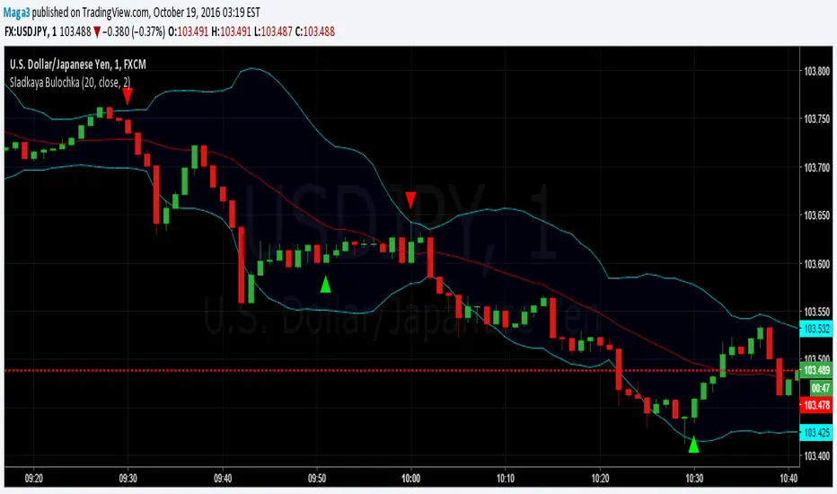
Sladkaya BulochkaAccording to the statistics of Thomas Bulkovski collected over several years on the 1-minute chart (21 million candles), there is a statistically significant periods, where the higher the probability of reversal rates on short-term timeframe.
By reversal, on average, had in mind the movement to 5 candles.
This three periods, they remain unchanged, depending on the hour:
- the first minute of each hour (10:01, 11:01, etc.)
- the first minute after the hour (10:31, 11:31)
- 51 minutes each hour (10:51, 11:51)
------------------------------------------------------
По статистике Томаса Булковски, собранной за несколько лет на 1-минутном графике (21 миллион свечей), есть статистически значимые периоды, где более высока вероятность разворота цены на краткосрочных ТФ.
Под разворотом, в среднем, имелось в виду движение на 5 свечей.
Это три периода, они неизменны в зависимости от часа:
- первая минута каждого часа (10:01, 11:01 и т.д.)
- первая минута после получаса (10:31, 11:31)
- каждая 51 минута часа (10:51, 11:51)
Get_rich_aggressively_v5# 🚀 GET RICH AGGRESSIVELY v5 - TIER SYSTEM
### Precision Futures Scalping | NQ • ES • YM • GC • BTC
### *Leave Every Trade With Money*
---
## 📋 QUICK CHEATSHEET
```
┌─────────────────────────────────────────────────────────────────────────────┐
│ GRA v5 SIGNAL REQUIREMENTS │
├─────────────────────────────────────────────────────────────────────────────┤
│ ✓ TIER MET Points ≥ 10 (B), ≥ 50 (A), ≥ 100 (S) │
│ ✓ VOLUME ≥ 1.3x average │
│ ✓ DELTA ≥ 55% dominance (buyers OR sellers) │
│ ✓ DIRECTION Candle color = Delta direction │
│ ✓ SESSION In London (3-5AM) or NY (9:30-11:30AM) if filter ON │
├─────────────────────────────────────────────────────────────────────────────┤
│ TIER ACTIONS │
├─────────────────────────────────────────────────────────────────────────────┤
│ 🥇 S-TIER (100+ pts) │ HOLD LONGER │ Big institutional move │
│ 🥈 A-TIER (50-99 pts) │ HOLD A BIT │ Medium move, trail to BE │
│ 🥉 B-TIER (10-49 pts) │ CLOSE QUICK │ Scalp 5-10 pts, exit fast │
│ ❌ NO TIER (< 10 pts) │ NO TRADE │ Not enough conviction │
├─────────────────────────────────────────────────────────────────────────────┤
│ SESSION PRIORITY │
├─────────────────────────────────────────────────────────────────────────────┤
│ 🔵 LONDON OPEN 03:00-05:00 ET │ IB forms 03:00-04:00 │
│ 🟢 NY OPEN 09:30-11:30 ET │ IB forms 09:30-10:30 │
│ 📊 IB BREAKOUT Close beyond IB + Impulse + 1.3x Vol = HIGH CONVICTION│
├─────────────────────────────────────────────────────────────────────────────┤
│ VOLUME PROFILE ZONES │
├─────────────────────────────────────────────────────────────────────────────┤
│ 🔵 HVN (Blue BG) High volume = Support/Resistance, expect consolidation │
│ 🟡 LVN (Yellow BG) Low volume = Breakout acceleration, fast moves │
│ 🟣 POC Point of Control = Institutional fair value │
│ 🟣 VAH/VAL Value Area edges = S/R zones │
├─────────────────────────────────────────────────────────────────────────────┤
│ MARKET STATE DECODER │
├─────────────────────────────────────────────────────────────────────────────┤
│ TREND UP │ Price > EMA20 + CVD rising │ Trade WITH the trend │
│ TREND DN │ Price < EMA20 + CVD falling │ Trade WITH the trend │
│ RETRACE │ Price/CVD diverging │ Pullback, prepare for entry │
│ RANGE │ No clear direction │ Reduce size or skip │
├─────────────────────────────────────────────────────────────────────────────┤
│ 💎 HIGH CONVICTION UPGRADE │
├─────────────────────────────────────────────────────────────────────────────┤
│ Purple diamond (◆) appears when: │
│ • Strong delta (≥65%) + Strong volume (≥2x) + Market in imbalance │
│ → Consider upgrading tier (B→A, A→S) for position sizing │
└─────────────────────────────────────────────────────────────────────────────┘
```
---
## 🎯 THE TIER SYSTEM
The tier system classifies candles by **point movement** to determine trade management:
| Tier | Points | Action | Expected R:R |
|:----:|:------:|:------:|:------------:|
| 🥇 **S-TIER** | 100+ | HOLD LONGER | 2:1+ |
| 🥈 **A-TIER** | 50-99 | HOLD A BIT | 1.5:1 |
| 🥉 **B-TIER** | 10-49 | CLOSE QUICK | 1:1 |
| ❌ **NO TIER** | < 10 | NO TRADE | — |
---
## ✅ SIGNAL REQUIREMENTS
**ALL conditions must be TRUE for a signal:**
```
SIGNAL = TIER + VOLUME + DELTA + DIRECTION + SESSION
☐ Points ≥ 10 (minimum B-tier)
☐ Volume ≥ 1.3x average
☐ Delta dominance ≥ 55%
☐ Candle direction = Delta direction
☐ In session (if filter ON)
ANY FALSE = NO SIGNAL = NO TRADE
```
---
## 📊 VOLUME DOMINANCE ANALYSIS
This is the **core edge** of GRA v5. We use intrabar analysis to determine who is in control:
```
VOLUME ANALYSIS BREAKDOWN
Total Volume = Buy Volume + Sell Volume
Buy Volume: Who pushed price UP within the bar
Sell Volume: Who pushed price DOWN within the bar
Delta = Buy Volume - Sell Volume
Buy Dominance = Buy Volume / Total Volume
Sell Dominance = Sell Volume / Total Volume
≥ 55% = ONE SIDE IN CONTROL
≥ 65% = STRONG DOMINANCE (high conviction)
```
**Direction Confirmation Matrix:**
| Candle | Delta | Signal |
|:-------|:------|:-------|
| 🟢 Bullish | 55%+ Buyers | ✅ LONG |
| 🟢 Bullish | 55%+ Sellers | ❌ Trap |
| 🔴 Bearish | 55%+ Sellers | ✅ SHORT |
| 🔴 Bearish | 55%+ Buyers | ❌ Trap |
---
## 🕐 SESSION CONTEXT
### Initial Balance (IB) Framework
The **first hour** of each session establishes the IB range. Institutions use this for the day's framework.
```
SESSION WINDOWS (Eastern Time):
LONDON:
├── IB Period: 03:00 - 04:00 ← Range established
├── Trade Window: 03:00 - 05:00 ← Best signals
└── Extension Targets: 1.5x, 2.0x
NY:
├── IB Period: 09:30 - 10:30 ← Range established
├── Trade Window: 09:30 - 11:30 ← Best signals
└── Extension Targets: 1.5x, 2.0x
```
### IB Breakout Signals
```
L▲ / L▼ = London IB Breakout (Blue)
N▲ / N▼ = NY IB Breakout (Orange)
Confirmation Required:
☐ Close beyond IB level (not just wick)
☐ Impulse candle (body > 60% of range)
☐ Volume > 1.3x average
```
**IB Statistics:**
- 97% of days break either IB high or low
- 1.5x extension = first profit target
- 2.0x extension = full range target
- ~66% of London sessions sweep Asian high/low first
---
## 📈 VIRTUAL VOLUME PROFILE ZONES
GRA v5 calculates volume profile zones **without drawing the profile**, giving you the key levels:
### Zone Types
| Zone | Background | Meaning | Action |
|:-----|:-----------|:--------|:-------|
| **HVN** | 🔵 Blue | High Volume Node | S/R zone, expect consolidation |
| **LVN** | 🟡 Yellow | Low Volume Node | Breakout zone, fast acceleration |
| **POC** | 🟣 Purple dots | Point of Control | Institutional fair value |
| **VAH/VAL** | 🟣 Purple lines | Value Area edges | S/R boundaries |
### How to Use
```
ENTERING A TRADE:
At HVN:
├── Expect price to consolidate
├── Look for rejection/absorption
└── Better for reversals
At LVN:
├── Expect fast price movement
├── Don't fight the direction
└── Better for breakouts
Near POC:
├── Institutional fair value
├── Strong magnet effect
└── Watch for volume at POC
```
---
## 🔄 MARKET STATE DETECTION
GRA v5 classifies the market into four states using **CVD + Price Action**:
```
CVD Direction
↑ Rising ↓ Falling
┌─────────────┬─────────────┐
Price > EMA20 │ TREND UP │ RETRACE │
│ (Go Long) │ (Pullback) │
├─────────────┼─────────────┤
Price < EMA20 │ RETRACE │ TREND DN │
│ (Pullback) │ (Go Short) │
└─────────────┴─────────────┘
```
| State | Meaning | Action |
|:------|:--------|:-------|
| **TREND UP** | Buyers in control | Trade long, follow signals |
| **TREND DN** | Sellers in control | Trade short, follow signals |
| **RETRACE** | Pullback against trend | Prepare for continuation entry |
| **RANGE** | No clear direction | Reduce size or wait |
---
## 💎 HIGH CONVICTION UPGRADES
When extra conditions align, GRA v5 marks the signal with a **purple diamond**:
```
HIGH CONVICTION = Base Signal + Strong Delta (65%+) + Strong Volume (2x+) + Imbalance State
```
**Action:** Consider upgrading tier for position sizing:
- B-Tier → A-Tier management
- A-Tier → S-Tier management
---
## 📋 TRADING BY TIER
### 🥇 S-TIER (100+ points)
| | |
|:--|:--|
| **Entry** | Candle close |
| **Target** | IB extension / Next S/R |
| **Management** | HOLD LONGER |
**Rules:**
- Watch next candle - continues? HOLD
- Same tier same direction? ADD
- Opposite tier signal? EXIT on close
- Never close early unless reversal signal
### 🥈 A-TIER (50-99 points)
| | |
|:--|:--|
| **Entry** | Candle close |
| **Target** | 1.5x initial risk minimum |
| **Management** | HOLD A BIT |
**Rules:**
- Target 1.5:1 R:R minimum
- Trail to breakeven after 1:1
- If stalls, take profit
- Upgrade to S-tier management if high conviction
### 🥉 B-TIER (10-49 points)
| | |
|:--|:--|
| **Entry** | Candle close |
| **Target** | 5-10 points MAX |
| **Management** | CLOSE QUICK |
**Rules:**
- Exit in 1-3 candles
- DO NOT hold for more
- Any doubt = EXIT
- Quick scalp mentality
---
## ⚙️ SETTINGS BY INSTRUMENT
| Setting | NQ/ES | YM | GC | BTC |
|:--------|:-----:|:--:|:--:|:---:|
| **Timeframe** | 1-5 min | 1-5 min | 5-15 min | 1-15 min |
| **S-Tier** | 100 pts | 100 pts | 15 pts | 500 pts |
| **A-Tier** | 50 pts | 50 pts | 8 pts | 250 pts |
| **B-Tier** | 10 pts | 15 pts | 3 pts | 50 pts |
| **Min Volume** | 1.3x | 1.3x | 1.5x | 1.3x |
| **Delta %** | 55% | 55% | 58% | 55% |
| **Best Time** | 9:30-11:30 ET | 9:30-11:30 ET | 3-5AM & 8:30-10:30 ET | 24/7 |
---
## 📊 TABLE LEGEND
The info panel displays real-time market data:
| Row | Shows | Colors |
|:----|:------|:-------|
| **Pts** | Candle points | Gold/Green/Yellow by tier |
| **Tier** | S/A/B/X | Gold/Green/Yellow/White |
| **Vol** | Volume ratio | Yellow (2x+) / Green (1.3x+) / Red |
| **Delta** | Buy/Sell % | Green (buy) / Red (sell) / White |
| **CVD** | Direction | Green ▲ / Red ▼ |
| **State** | Market state | Green/Red/Orange/Gray |
| **Sess** | Session | Yellow if active |
| **Zone** | VP zone | Blue/Yellow/Purple |
| **Sig** | Signal | Green/Red if active |
---
## 🔔 ALERTS
| Alert | When | Action |
|:------|:-----|:-------|
| **S-TIER LONG/SHORT** | S-tier signal | Hold longer |
| **A-TIER LONG/SHORT** | A-tier signal | Hold a bit |
| **B-TIER LONG/SHORT** | B-tier signal | Close quick |
| **LON IB BREAK UP/DN** | London IB breakout | Major session move |
| **NY IB BREAK UP/DN** | NY IB breakout | Major session move |
| **HIGH CONVICTION** | Upgraded signal | Consider larger size |
| **LONDON/NY OPEN** | Session start | Get ready |
---
## 💰 THE GOLDEN RULE
> ### **LEAVE EVERY TRADE WITH MONEY**
>
> | Situation | Rule |
> |:----------|:-----|
> | B-Tier | Small win > Small loss |
> | A-Tier | Trail to BE, lock profit |
> | S-Tier | Let it run to target |
> | No Signal | NO TRADE |
> | Wrong Side | EXIT immediately |
>
> **Capital preserved = Trade tomorrow**
---
## ⚠️ DISCLAIMER
> Risk management is **YOUR** responsibility.
> Never risk more than 1-2% per trade.
> Paper trade until you understand the signals.
> Past performance ≠ future results.
---
### Get Rich. Stay Rich. Trade Aggressively. 🚀
**Get Rich Aggressively v5**
*Precision Futures Scalping*

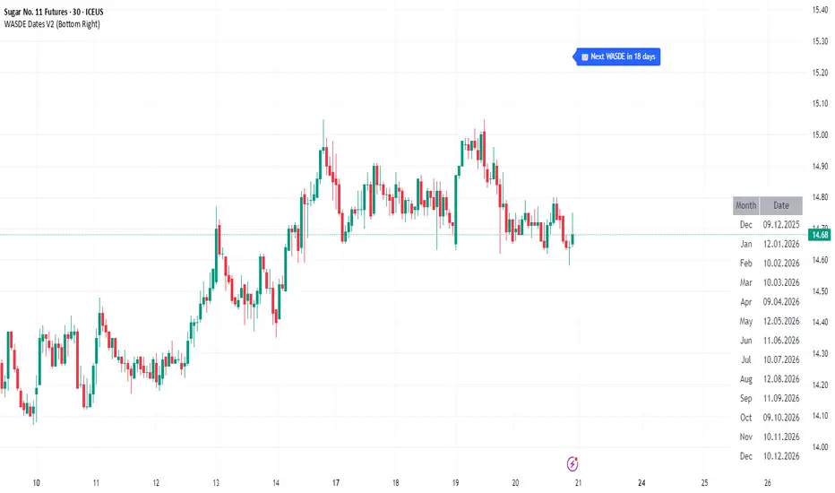
WASDE Dates V2WASDE Dates V2 – USDA Release Calendar with Alerts, Countdown & Event Markers
By cot-trader.com
WASDE Dates V2 is a complete and reliable visualization tool for all scheduled WASDE (World Agricultural Supply and Demand Estimates) releases for 2025 and 2026.
The USDA’s WASDE report is one of the most market-moving fundamental catalysts in agricultural futures—affecting Corn (ZC), Wheat (ZW), Soybeans (ZS), Soymeal (ZM), Soybean Oil (ZL), and many related CFD products.
This script gives traders a precise timing layer directly inside their TradingView charts.
🔍 What this script does
WASDE Dates V2 automatically:
Marks each WASDE release day with a vertical line and label.
Shows an automated countdown to the next WASDE release:
In days (>24h)
In hours & minutes (<24h)
Displays an optional table of upcoming WASDE dates for quick reference.
Provides two alert conditions:
WASDE Day Alert – triggers exactly on the event
WASDE 24h Reminder – pre-alert when less than 24 hours remain
Handles both 2025 and 2026 confirmed dates.
Works on any symbol and timeframe.
📌 Why WASDE matters
The WASDE report updates global supply and demand estimates for:
Corn
Soybeans
Wheat
Other major agricultural commodities
Changes in yield, acres, production, imports/exports, and ending stocks can cause immediate and significant volatility.
Many traders combine WASDE awareness with seasonality, COT positioning, volatility filters, or fundamental models.
This script ensures you never miss the timing of these key releases.
⚙️ How the script works
The script stores official USDA WASDE release dates for 2025 and 2026 in two dedicated arrays.
On every bar, it compares the bar’s timestamp with known WASDE timestamps to detect an event day.
When an event occurs:
A red “WASDE” label is plotted above the candle
A dotted vertical line is drawn through the bar
It finds the next upcoming WASDE by scanning forward through both arrays.
A live-updating countdown label is displayed, showing days or hours/minutes until release.
If the event is less than 24 hours away:
A yellow “WASDE soon” warning appears near price
The 24h alert condition becomes active
An optional table lists upcoming events for 2025 & 2026.
This script does not generate trading signals.
It provides a time-based event layer designed to complement any discretionary or algorithmic trading approach.
🧭 How to use
Add the script to your chart.
Enable alerts for:
“WASDE Day Alert”
“WASDE 24h Reminder”
Follow the countdown to prepare for upcoming volatility.
Use together with other agricultural tools such as:
Seasonality indicators
COT (Commitment of Traders) analysis
Trend / VWAP / Volume signals
Pre- and post-WASDE trading strategies
Works on all chart types, all symbols, and all timeframes.
📅 Included WASDE Dates (Confirmed)
2025:
Jan 12, Feb 11, Mar 11, Apr 10, May 12, Jun 12, Jul 11, Aug 12, Sep 12, Oct 9, Nov 10, Dec 9
2026:
Jan 12, Feb 10, Mar 10, Apr 9, May 12, Jun 11, Jul 10, Aug 12, Sep 11, Oct 9, Nov 10, Dec 10
(All dates based on USDA’s official 12:00pm ET schedule.)
💡 What makes this script original
Fully updated 2025 + 2026 calendar
Uses a robust time-comparison method for accurate marking
Unique dual alert system (event + 24h pre-alert)
Clean, readable layout with countdown + upcoming dates table
Tailored specifically for grain & agricultural traders
Built entirely in Pine Script v6 with careful attention to performance
Markov Chain [3D] | FractalystWhat exactly is a Markov Chain?
This indicator uses a Markov Chain model to analyze, quantify, and visualize the transitions between market regimes (Bull, Bear, Neutral) on your chart. It dynamically detects these regimes in real-time, calculates transition probabilities, and displays them as animated 3D spheres and arrows, giving traders intuitive insight into current and future market conditions.
How does a Markov Chain work, and how should I read this spheres-and-arrows diagram?
Think of three weather modes: Sunny, Rainy, Cloudy.
Each sphere is one mode. The loop on a sphere means “stay the same next step” (e.g., Sunny again tomorrow).
The arrows leaving a sphere show where things usually go next if they change (e.g., Sunny moving to Cloudy).
Some paths matter more than others. A more prominent loop means the current mode tends to persist. A more prominent outgoing arrow means a change to that destination is the usual next step.
Direction isn’t symmetric: moving Sunny→Cloudy can behave differently than Cloudy→Sunny.
Now relabel the spheres to markets: Bull, Bear, Neutral.
Spheres: market regimes (uptrend, downtrend, range).
Self‑loop: tendency for the current regime to continue on the next bar.
Arrows: the most common next regime if a switch happens.
How to read: Start at the sphere that matches current bar state. If the loop stands out, expect continuation. If one outgoing path stands out, that switch is the typical next step. Opposite directions can differ (Bear→Neutral doesn’t have to match Neutral→Bear).
What states and transitions are shown?
The three market states visualized are:
Bullish (Bull): Upward or strong-market regime.
Bearish (Bear): Downward or weak-market regime.
Neutral: Sideways or range-bound regime.
Bidirectional animated arrows and probability labels show how likely the market is to move from one regime to another (e.g., Bull → Bear or Neutral → Bull).
How does the regime detection system work?
You can use either built-in price returns (based on adaptive Z-score normalization) or supply three custom indicators (such as volume, oscillators, etc.).
Values are statistically normalized (Z-scored) over a configurable lookback period.
The normalized outputs are classified into Bull, Bear, or Neutral zones.
If using three indicators, their regime signals are averaged and smoothed for robustness.
How are transition probabilities calculated?
On every confirmed bar, the algorithm tracks the sequence of detected market states, then builds a rolling window of transitions.
The code maintains a transition count matrix for all regime pairs (e.g., Bull → Bear).
Transition probabilities are extracted for each possible state change using Laplace smoothing for numerical stability, and frequently updated in real-time.
What is unique about the visualization?
3D animated spheres represent each regime and change visually when active.
Animated, bidirectional arrows reveal transition probabilities and allow you to see both dominant and less likely regime flows.
Particles (moving dots) animate along the arrows, enhancing the perception of regime flow direction and speed.
All elements dynamically update with each new price bar, providing a live market map in an intuitive, engaging format.
Can I use custom indicators for regime classification?
Yes! Enable the "Custom Indicators" switch and select any three chart series as inputs. These will be normalized and combined (each with equal weight), broadening the regime classification beyond just price-based movement.
What does the “Lookback Period” control?
Lookback Period (default: 100) sets how much historical data builds the probability matrix. Shorter periods adapt faster to regime changes but may be noisier. Longer periods are more stable but slower to adapt.
How is this different from a Hidden Markov Model (HMM)?
It sets the window for both regime detection and probability calculations. Lower values make the system more reactive, but potentially noisier. Higher values smooth estimates and make the system more robust.
How is this Markov Chain different from a Hidden Markov Model (HMM)?
Markov Chain (as here): All market regimes (Bull, Bear, Neutral) are directly observable on the chart. The transition matrix is built from actual detected regimes, keeping the model simple and interpretable.
Hidden Markov Model: The actual regimes are unobservable ("hidden") and must be inferred from market output or indicator "emissions" using statistical learning algorithms. HMMs are more complex, can capture more subtle structure, but are harder to visualize and require additional machine learning steps for training.
A standard Markov Chain models transitions between observable states using a simple transition matrix, while a Hidden Markov Model assumes the true states are hidden (latent) and must be inferred from observable “emissions” like price or volume data. In practical terms, a Markov Chain is transparent and easier to implement and interpret; an HMM is more expressive but requires statistical inference to estimate hidden states from data.
Markov Chain: states are observable; you directly count or estimate transition probabilities between visible states. This makes it simpler, faster, and easier to validate and tune.
HMM: states are hidden; you only observe emissions generated by those latent states. Learning involves machine learning/statistical algorithms (commonly Baum–Welch/EM for training and Viterbi for decoding) to infer both the transition dynamics and the most likely hidden state sequence from data.
How does the indicator avoid “repainting” or look-ahead bias?
All regime changes and matrix updates happen only on confirmed (closed) bars, so no future data is leaked, ensuring reliable real-time operation.
Are there practical tuning tips?
Tune the Lookback Period for your asset/timeframe: shorter for fast markets, longer for stability.
Use custom indicators if your asset has unique regime drivers.
Watch for rapid changes in transition probabilities as early warning of a possible regime shift.
Who is this indicator for?
Quants and quantitative researchers exploring probabilistic market modeling, especially those interested in regime-switching dynamics and Markov models.
Programmers and system developers who need a probabilistic regime filter for systematic and algorithmic backtesting:
The Markov Chain indicator is ideally suited for programmatic integration via its bias output (1 = Bull, 0 = Neutral, -1 = Bear).
Although the visualization is engaging, the core output is designed for automated, rules-based workflows—not for discretionary/manual trading decisions.
Developers can connect the indicator’s output directly to their Pine Script logic (using input.source()), allowing rapid and robust backtesting of regime-based strategies.
It acts as a plug-and-play regime filter: simply plug the bias output into your entry/exit logic, and you have a scientifically robust, probabilistically-derived signal for filtering, timing, position sizing, or risk regimes.
The MC's output is intentionally "trinary" (1/0/-1), focusing on clear regime states for unambiguous decision-making in code. If you require nuanced, multi-probability or soft-label state vectors, consider expanding the indicator or stacking it with a probability-weighted logic layer in your scripting.
Because it avoids subjectivity, this approach is optimal for systematic quants, algo developers building backtested, repeatable strategies based on probabilistic regime analysis.
What's the mathematical foundation behind this?
The mathematical foundation behind this Markov Chain indicator—and probabilistic regime detection in finance—draws from two principal models: the (standard) Markov Chain and the Hidden Markov Model (HMM).
How to use this indicator programmatically?
The Markov Chain indicator automatically exports a bias value (+1 for Bullish, -1 for Bearish, 0 for Neutral) as a plot visible in the Data Window. This allows you to integrate its regime signal into your own scripts and strategies for backtesting, automation, or live trading.
Step-by-Step Integration with Pine Script (input.source)
Add the Markov Chain indicator to your chart.
This must be done first, since your custom script will "pull" the bias signal from the indicator's plot.
In your strategy, create an input using input.source()
Example:
//@version=5
strategy("MC Bias Strategy Example")
mcBias = input.source(close, "MC Bias Source")
After saving, go to your script’s settings. For the “MC Bias Source” input, select the plot/output of the Markov Chain indicator (typically its bias plot).
Use the bias in your trading logic
Example (long only on Bull, flat otherwise):
if mcBias == 1
strategy.entry("Long", strategy.long)
else
strategy.close("Long")
For more advanced workflows, combine mcBias with additional filters or trailing stops.
How does this work behind-the-scenes?
TradingView’s input.source() lets you use any plot from another indicator as a real-time, “live” data feed in your own script (source).
The selected bias signal is available to your Pine code as a variable, enabling logical decisions based on regime (trend-following, mean-reversion, etc.).
This enables powerful strategy modularity : decouple regime detection from entry/exit logic, allowing fast experimentation without rewriting core signal code.
Integrating 45+ Indicators with Your Markov Chain — How & Why
The Enhanced Custom Indicators Export script exports a massive suite of over 45 technical indicators—ranging from classic momentum (RSI, MACD, Stochastic, etc.) to trend, volume, volatility, and oscillator tools—all pre-calculated, centered/scaled, and available as plots.
// Enhanced Custom Indicators Export - 45 Technical Indicators
// Comprehensive technical analysis suite for advanced market regime detection
//@version=6
indicator('Enhanced Custom Indicators Export | Fractalyst', shorttitle='Enhanced CI Export', overlay=false, scale=scale.right, max_labels_count=500, max_lines_count=500)
// |----- Input Parameters -----| //
momentum_group = "Momentum Indicators"
trend_group = "Trend Indicators"
volume_group = "Volume Indicators"
volatility_group = "Volatility Indicators"
oscillator_group = "Oscillator Indicators"
display_group = "Display Settings"
// Common lengths
length_14 = input.int(14, "Standard Length (14)", minval=1, maxval=100, group=momentum_group)
length_20 = input.int(20, "Medium Length (20)", minval=1, maxval=200, group=trend_group)
length_50 = input.int(50, "Long Length (50)", minval=1, maxval=200, group=trend_group)
// Display options
show_table = input.bool(true, "Show Values Table", group=display_group)
table_size = input.string("Small", "Table Size", options= , group=display_group)
// |----- MOMENTUM INDICATORS (15 indicators) -----| //
// 1. RSI (Relative Strength Index)
rsi_14 = ta.rsi(close, length_14)
rsi_centered = rsi_14 - 50
// 2. Stochastic Oscillator
stoch_k = ta.stoch(close, high, low, length_14)
stoch_d = ta.sma(stoch_k, 3)
stoch_centered = stoch_k - 50
// 3. Williams %R
williams_r = ta.stoch(close, high, low, length_14) - 100
// 4. MACD (Moving Average Convergence Divergence)
= ta.macd(close, 12, 26, 9)
// 5. Momentum (Rate of Change)
momentum = ta.mom(close, length_14)
momentum_pct = (momentum / close ) * 100
// 6. Rate of Change (ROC)
roc = ta.roc(close, length_14)
// 7. Commodity Channel Index (CCI)
cci = ta.cci(close, length_20)
// 8. Money Flow Index (MFI)
mfi = ta.mfi(close, length_14)
mfi_centered = mfi - 50
// 9. Awesome Oscillator (AO)
ao = ta.sma(hl2, 5) - ta.sma(hl2, 34)
// 10. Accelerator Oscillator (AC)
ac = ao - ta.sma(ao, 5)
// 11. Chande Momentum Oscillator (CMO)
cmo = ta.cmo(close, length_14)
// 12. Detrended Price Oscillator (DPO)
dpo = close - ta.sma(close, length_20)
// 13. Price Oscillator (PPO)
ppo = ta.sma(close, 12) - ta.sma(close, 26)
ppo_pct = (ppo / ta.sma(close, 26)) * 100
// 14. TRIX
trix_ema1 = ta.ema(close, length_14)
trix_ema2 = ta.ema(trix_ema1, length_14)
trix_ema3 = ta.ema(trix_ema2, length_14)
trix = ta.roc(trix_ema3, 1) * 10000
// 15. Klinger Oscillator
klinger = ta.ema(volume * (high + low + close) / 3, 34) - ta.ema(volume * (high + low + close) / 3, 55)
// 16. Fisher Transform
fisher_hl2 = 0.5 * (hl2 - ta.lowest(hl2, 10)) / (ta.highest(hl2, 10) - ta.lowest(hl2, 10)) - 0.25
fisher = 0.5 * math.log((1 + fisher_hl2) / (1 - fisher_hl2))
// 17. Stochastic RSI
stoch_rsi = ta.stoch(rsi_14, rsi_14, rsi_14, length_14)
stoch_rsi_centered = stoch_rsi - 50
// 18. Relative Vigor Index (RVI)
rvi_num = ta.swma(close - open)
rvi_den = ta.swma(high - low)
rvi = rvi_den != 0 ? rvi_num / rvi_den : 0
// 19. Balance of Power (BOP)
bop = (close - open) / (high - low)
// |----- TREND INDICATORS (10 indicators) -----| //
// 20. Simple Moving Average Momentum
sma_20 = ta.sma(close, length_20)
sma_momentum = ((close - sma_20) / sma_20) * 100
// 21. Exponential Moving Average Momentum
ema_20 = ta.ema(close, length_20)
ema_momentum = ((close - ema_20) / ema_20) * 100
// 22. Parabolic SAR
sar = ta.sar(0.02, 0.02, 0.2)
sar_trend = close > sar ? 1 : -1
// 23. Linear Regression Slope
lr_slope = ta.linreg(close, length_20, 0) - ta.linreg(close, length_20, 1)
// 24. Moving Average Convergence (MAC)
mac = ta.sma(close, 10) - ta.sma(close, 30)
// 25. Trend Intensity Index (TII)
tii_sum = 0.0
for i = 1 to length_20
tii_sum += close > close ? 1 : 0
tii = (tii_sum / length_20) * 100
// 26. Ichimoku Cloud Components
ichimoku_tenkan = (ta.highest(high, 9) + ta.lowest(low, 9)) / 2
ichimoku_kijun = (ta.highest(high, 26) + ta.lowest(low, 26)) / 2
ichimoku_signal = ichimoku_tenkan > ichimoku_kijun ? 1 : -1
// 27. MESA Adaptive Moving Average (MAMA)
mama_alpha = 2.0 / (length_20 + 1)
mama = ta.ema(close, length_20)
mama_momentum = ((close - mama) / mama) * 100
// 28. Zero Lag Exponential Moving Average (ZLEMA)
zlema_lag = math.round((length_20 - 1) / 2)
zlema_data = close + (close - close )
zlema = ta.ema(zlema_data, length_20)
zlema_momentum = ((close - zlema) / zlema) * 100
// |----- VOLUME INDICATORS (6 indicators) -----| //
// 29. On-Balance Volume (OBV)
obv = ta.obv
// 30. Volume Rate of Change (VROC)
vroc = ta.roc(volume, length_14)
// 31. Price Volume Trend (PVT)
pvt = ta.pvt
// 32. Negative Volume Index (NVI)
nvi = 0.0
nvi := volume < volume ? nvi + ((close - close ) / close ) * nvi : nvi
// 33. Positive Volume Index (PVI)
pvi = 0.0
pvi := volume > volume ? pvi + ((close - close ) / close ) * pvi : pvi
// 34. Volume Oscillator
vol_osc = ta.sma(volume, 5) - ta.sma(volume, 10)
// 35. Ease of Movement (EOM)
eom_distance = high - low
eom_box_height = volume / 1000000
eom = eom_box_height != 0 ? eom_distance / eom_box_height : 0
eom_sma = ta.sma(eom, length_14)
// 36. Force Index
force_index = volume * (close - close )
force_index_sma = ta.sma(force_index, length_14)
// |----- VOLATILITY INDICATORS (10 indicators) -----| //
// 37. Average True Range (ATR)
atr = ta.atr(length_14)
atr_pct = (atr / close) * 100
// 38. Bollinger Bands Position
bb_basis = ta.sma(close, length_20)
bb_dev = 2.0 * ta.stdev(close, length_20)
bb_upper = bb_basis + bb_dev
bb_lower = bb_basis - bb_dev
bb_position = bb_dev != 0 ? (close - bb_basis) / bb_dev : 0
bb_width = bb_dev != 0 ? (bb_upper - bb_lower) / bb_basis * 100 : 0
// 39. Keltner Channels Position
kc_basis = ta.ema(close, length_20)
kc_range = ta.ema(ta.tr, length_20)
kc_upper = kc_basis + (2.0 * kc_range)
kc_lower = kc_basis - (2.0 * kc_range)
kc_position = kc_range != 0 ? (close - kc_basis) / kc_range : 0
// 40. Donchian Channels Position
dc_upper = ta.highest(high, length_20)
dc_lower = ta.lowest(low, length_20)
dc_basis = (dc_upper + dc_lower) / 2
dc_position = (dc_upper - dc_lower) != 0 ? (close - dc_basis) / (dc_upper - dc_lower) : 0
// 41. Standard Deviation
std_dev = ta.stdev(close, length_20)
std_dev_pct = (std_dev / close) * 100
// 42. Relative Volatility Index (RVI)
rvi_up = ta.stdev(close > close ? close : 0, length_14)
rvi_down = ta.stdev(close < close ? close : 0, length_14)
rvi_total = rvi_up + rvi_down
rvi_volatility = rvi_total != 0 ? (rvi_up / rvi_total) * 100 : 50
// 43. Historical Volatility
hv_returns = math.log(close / close )
hv = ta.stdev(hv_returns, length_20) * math.sqrt(252) * 100
// 44. Garman-Klass Volatility
gk_vol = math.log(high/low) * math.log(high/low) - (2*math.log(2)-1) * math.log(close/open) * math.log(close/open)
gk_volatility = math.sqrt(ta.sma(gk_vol, length_20)) * 100
// 45. Parkinson Volatility
park_vol = math.log(high/low) * math.log(high/low)
parkinson = math.sqrt(ta.sma(park_vol, length_20) / (4 * math.log(2))) * 100
// 46. Rogers-Satchell Volatility
rs_vol = math.log(high/close) * math.log(high/open) + math.log(low/close) * math.log(low/open)
rogers_satchell = math.sqrt(ta.sma(rs_vol, length_20)) * 100
// |----- OSCILLATOR INDICATORS (5 indicators) -----| //
// 47. Elder Ray Index
elder_bull = high - ta.ema(close, 13)
elder_bear = low - ta.ema(close, 13)
elder_power = elder_bull + elder_bear
// 48. Schaff Trend Cycle (STC)
stc_macd = ta.ema(close, 23) - ta.ema(close, 50)
stc_k = ta.stoch(stc_macd, stc_macd, stc_macd, 10)
stc_d = ta.ema(stc_k, 3)
stc = ta.stoch(stc_d, stc_d, stc_d, 10)
// 49. Coppock Curve
coppock_roc1 = ta.roc(close, 14)
coppock_roc2 = ta.roc(close, 11)
coppock = ta.wma(coppock_roc1 + coppock_roc2, 10)
// 50. Know Sure Thing (KST)
kst_roc1 = ta.roc(close, 10)
kst_roc2 = ta.roc(close, 15)
kst_roc3 = ta.roc(close, 20)
kst_roc4 = ta.roc(close, 30)
kst = ta.sma(kst_roc1, 10) + 2*ta.sma(kst_roc2, 10) + 3*ta.sma(kst_roc3, 10) + 4*ta.sma(kst_roc4, 15)
// 51. Percentage Price Oscillator (PPO)
ppo_line = ((ta.ema(close, 12) - ta.ema(close, 26)) / ta.ema(close, 26)) * 100
ppo_signal = ta.ema(ppo_line, 9)
ppo_histogram = ppo_line - ppo_signal
// |----- PLOT MAIN INDICATORS -----| //
// Plot key momentum indicators
plot(rsi_centered, title="01_RSI_Centered", color=color.purple, linewidth=1)
plot(stoch_centered, title="02_Stoch_Centered", color=color.blue, linewidth=1)
plot(williams_r, title="03_Williams_R", color=color.red, linewidth=1)
plot(macd_histogram, title="04_MACD_Histogram", color=color.orange, linewidth=1)
plot(cci, title="05_CCI", color=color.green, linewidth=1)
// Plot trend indicators
plot(sma_momentum, title="06_SMA_Momentum", color=color.navy, linewidth=1)
plot(ema_momentum, title="07_EMA_Momentum", color=color.maroon, linewidth=1)
plot(sar_trend, title="08_SAR_Trend", color=color.teal, linewidth=1)
plot(lr_slope, title="09_LR_Slope", color=color.lime, linewidth=1)
plot(mac, title="10_MAC", color=color.fuchsia, linewidth=1)
// Plot volatility indicators
plot(atr_pct, title="11_ATR_Pct", color=color.yellow, linewidth=1)
plot(bb_position, title="12_BB_Position", color=color.aqua, linewidth=1)
plot(kc_position, title="13_KC_Position", color=color.olive, linewidth=1)
plot(std_dev_pct, title="14_StdDev_Pct", color=color.silver, linewidth=1)
plot(bb_width, title="15_BB_Width", color=color.gray, linewidth=1)
// Plot volume indicators
plot(vroc, title="16_VROC", color=color.blue, linewidth=1)
plot(eom_sma, title="17_EOM", color=color.red, linewidth=1)
plot(vol_osc, title="18_Vol_Osc", color=color.green, linewidth=1)
plot(force_index_sma, title="19_Force_Index", color=color.orange, linewidth=1)
plot(obv, title="20_OBV", color=color.purple, linewidth=1)
// Plot additional oscillators
plot(ao, title="21_Awesome_Osc", color=color.navy, linewidth=1)
plot(cmo, title="22_CMO", color=color.maroon, linewidth=1)
plot(dpo, title="23_DPO", color=color.teal, linewidth=1)
plot(trix, title="24_TRIX", color=color.lime, linewidth=1)
plot(fisher, title="25_Fisher", color=color.fuchsia, linewidth=1)
// Plot more momentum indicators
plot(mfi_centered, title="26_MFI_Centered", color=color.yellow, linewidth=1)
plot(ac, title="27_AC", color=color.aqua, linewidth=1)
plot(ppo_pct, title="28_PPO_Pct", color=color.olive, linewidth=1)
plot(stoch_rsi_centered, title="29_StochRSI_Centered", color=color.silver, linewidth=1)
plot(klinger, title="30_Klinger", color=color.gray, linewidth=1)
// Plot trend continuation
plot(tii, title="31_TII", color=color.blue, linewidth=1)
plot(ichimoku_signal, title="32_Ichimoku_Signal", color=color.red, linewidth=1)
plot(mama_momentum, title="33_MAMA_Momentum", color=color.green, linewidth=1)
plot(zlema_momentum, title="34_ZLEMA_Momentum", color=color.orange, linewidth=1)
plot(bop, title="35_BOP", color=color.purple, linewidth=1)
// Plot volume continuation
plot(nvi, title="36_NVI", color=color.navy, linewidth=1)
plot(pvi, title="37_PVI", color=color.maroon, linewidth=1)
plot(momentum_pct, title="38_Momentum_Pct", color=color.teal, linewidth=1)
plot(roc, title="39_ROC", color=color.lime, linewidth=1)
plot(rvi, title="40_RVI", color=color.fuchsia, linewidth=1)
// Plot volatility continuation
plot(dc_position, title="41_DC_Position", color=color.yellow, linewidth=1)
plot(rvi_volatility, title="42_RVI_Volatility", color=color.aqua, linewidth=1)
plot(hv, title="43_Historical_Vol", color=color.olive, linewidth=1)
plot(gk_volatility, title="44_GK_Volatility", color=color.silver, linewidth=1)
plot(parkinson, title="45_Parkinson_Vol", color=color.gray, linewidth=1)
// Plot final oscillators
plot(rogers_satchell, title="46_RS_Volatility", color=color.blue, linewidth=1)
plot(elder_power, title="47_Elder_Power", color=color.red, linewidth=1)
plot(stc, title="48_STC", color=color.green, linewidth=1)
plot(coppock, title="49_Coppock", color=color.orange, linewidth=1)
plot(kst, title="50_KST", color=color.purple, linewidth=1)
// Plot final indicators
plot(ppo_histogram, title="51_PPO_Histogram", color=color.navy, linewidth=1)
plot(pvt, title="52_PVT", color=color.maroon, linewidth=1)
// |----- Reference Lines -----| //
hline(0, "Zero Line", color=color.gray, linestyle=hline.style_dashed, linewidth=1)
hline(50, "Midline", color=color.gray, linestyle=hline.style_dotted, linewidth=1)
hline(-50, "Lower Midline", color=color.gray, linestyle=hline.style_dotted, linewidth=1)
hline(25, "Upper Threshold", color=color.gray, linestyle=hline.style_dotted, linewidth=1)
hline(-25, "Lower Threshold", color=color.gray, linestyle=hline.style_dotted, linewidth=1)
// |----- Enhanced Information Table -----| //
if show_table and barstate.islast
table_position = position.top_right
table_text_size = table_size == "Tiny" ? size.tiny : table_size == "Small" ? size.small : size.normal
var table info_table = table.new(table_position, 3, 18, bgcolor=color.new(color.white, 85), border_width=1, border_color=color.gray)
// Headers
table.cell(info_table, 0, 0, 'Category', text_color=color.black, text_size=table_text_size, bgcolor=color.new(color.blue, 70))
table.cell(info_table, 1, 0, 'Indicator', text_color=color.black, text_size=table_text_size, bgcolor=color.new(color.blue, 70))
table.cell(info_table, 2, 0, 'Value', text_color=color.black, text_size=table_text_size, bgcolor=color.new(color.blue, 70))
// Key Momentum Indicators
table.cell(info_table, 0, 1, 'MOMENTUM', text_color=color.purple, text_size=table_text_size, bgcolor=color.new(color.purple, 90))
table.cell(info_table, 1, 1, 'RSI Centered', text_color=color.purple, text_size=table_text_size)
table.cell(info_table, 2, 1, str.tostring(rsi_centered, '0.00'), text_color=color.purple, text_size=table_text_size)
table.cell(info_table, 0, 2, '', text_color=color.blue, text_size=table_text_size)
table.cell(info_table, 1, 2, 'Stoch Centered', text_color=color.blue, text_size=table_text_size)
table.cell(info_table, 2, 2, str.tostring(stoch_centered, '0.00'), text_color=color.blue, text_size=table_text_size)
table.cell(info_table, 0, 3, '', text_color=color.red, text_size=table_text_size)
table.cell(info_table, 1, 3, 'Williams %R', text_color=color.red, text_size=table_text_size)
table.cell(info_table, 2, 3, str.tostring(williams_r, '0.00'), text_color=color.red, text_size=table_text_size)
table.cell(info_table, 0, 4, '', text_color=color.orange, text_size=table_text_size)
table.cell(info_table, 1, 4, 'MACD Histogram', text_color=color.orange, text_size=table_text_size)
table.cell(info_table, 2, 4, str.tostring(macd_histogram, '0.000'), text_color=color.orange, text_size=table_text_size)
table.cell(info_table, 0, 5, '', text_color=color.green, text_size=table_text_size)
table.cell(info_table, 1, 5, 'CCI', text_color=color.green, text_size=table_text_size)
table.cell(info_table, 2, 5, str.tostring(cci, '0.00'), text_color=color.green, text_size=table_text_size)
// Key Trend Indicators
table.cell(info_table, 0, 6, 'TREND', text_color=color.navy, text_size=table_text_size, bgcolor=color.new(color.navy, 90))
table.cell(info_table, 1, 6, 'SMA Momentum %', text_color=color.navy, text_size=table_text_size)
table.cell(info_table, 2, 6, str.tostring(sma_momentum, '0.00'), text_color=color.navy, text_size=table_text_size)
table.cell(info_table, 0, 7, '', text_color=color.maroon, text_size=table_text_size)
table.cell(info_table, 1, 7, 'EMA Momentum %', text_color=color.maroon, text_size=table_text_size)
table.cell(info_table, 2, 7, str.tostring(ema_momentum, '0.00'), text_color=color.maroon, text_size=table_text_size)
table.cell(info_table, 0, 8, '', text_color=color.teal, text_size=table_text_size)
table.cell(info_table, 1, 8, 'SAR Trend', text_color=color.teal, text_size=table_text_size)
table.cell(info_table, 2, 8, str.tostring(sar_trend, '0'), text_color=color.teal, text_size=table_text_size)
table.cell(info_table, 0, 9, '', text_color=color.lime, text_size=table_text_size)
table.cell(info_table, 1, 9, 'Linear Regression', text_color=color.lime, text_size=table_text_size)
table.cell(info_table, 2, 9, str.tostring(lr_slope, '0.000'), text_color=color.lime, text_size=table_text_size)
// Key Volatility Indicators
table.cell(info_table, 0, 10, 'VOLATILITY', text_color=color.yellow, text_size=table_text_size, bgcolor=color.new(color.yellow, 90))
table.cell(info_table, 1, 10, 'ATR %', text_color=color.yellow, text_size=table_text_size)
table.cell(info_table, 2, 10, str.tostring(atr_pct, '0.00'), text_color=color.yellow, text_size=table_text_size)
table.cell(info_table, 0, 11, '', text_color=color.aqua, text_size=table_text_size)
table.cell(info_table, 1, 11, 'BB Position', text_color=color.aqua, text_size=table_text_size)
table.cell(info_table, 2, 11, str.tostring(bb_position, '0.00'), text_color=color.aqua, text_size=table_text_size)
table.cell(info_table, 0, 12, '', text_color=color.olive, text_size=table_text_size)
table.cell(info_table, 1, 12, 'KC Position', text_color=color.olive, text_size=table_text_size)
table.cell(info_table, 2, 12, str.tostring(kc_position, '0.00'), text_color=color.olive, text_size=table_text_size)
// Key Volume Indicators
table.cell(info_table, 0, 13, 'VOLUME', text_color=color.blue, text_size=table_text_size, bgcolor=color.new(color.blue, 90))
table.cell(info_table, 1, 13, 'Volume ROC', text_color=color.blue, text_size=table_text_size)
table.cell(info_table, 2, 13, str.tostring(vroc, '0.00'), text_color=color.blue, text_size=table_text_size)
table.cell(info_table, 0, 14, '', text_color=color.red, text_size=table_text_size)
table.cell(info_table, 1, 14, 'EOM', text_color=color.red, text_size=table_text_size)
table.cell(info_table, 2, 14, str.tostring(eom_sma, '0.000'), text_color=color.red, text_size=table_text_size)
// Key Oscillators
table.cell(info_table, 0, 15, 'OSCILLATORS', text_color=color.purple, text_size=table_text_size, bgcolor=color.new(color.purple, 90))
table.cell(info_table, 1, 15, 'Awesome Osc', text_color=color.blue, text_size=table_text_size)
table.cell(info_table, 2, 15, str.tostring(ao, '0.000'), text_color=color.blue, text_size=table_text_size)
table.cell(info_table, 0, 16, '', text_color=color.red, text_size=table_text_size)
table.cell(info_table, 1, 16, 'Fisher Transform', text_color=color.red, text_size=table_text_size)
table.cell(info_table, 2, 16, str.tostring(fisher, '0.000'), text_color=color.red, text_size=table_text_size)
// Summary Statistics
table.cell(info_table, 0, 17, 'SUMMARY', text_color=color.black, text_size=table_text_size, bgcolor=color.new(color.gray, 70))
table.cell(info_table, 1, 17, 'Total Indicators: 52', text_color=color.black, text_size=table_text_size)
regime_color = rsi_centered > 10 ? color.green : rsi_centered < -10 ? color.red : color.gray
regime_text = rsi_centered > 10 ? "BULLISH" : rsi_centered < -10 ? "BEARISH" : "NEUTRAL"
table.cell(info_table, 2, 17, regime_text, text_color=regime_color, text_size=table_text_size)
This makes it the perfect “indicator backbone” for quantitative and systematic traders who want to prototype, combine, and test new regime detection models—especially in combination with the Markov Chain indicator.
How to use this script with the Markov Chain for research and backtesting:
Add the Enhanced Indicator Export to your chart.
Every calculated indicator is available as an individual data stream.
Connect the indicator(s) you want as custom input(s) to the Markov Chain’s “Custom Indicators” option.
In the Markov Chain indicator’s settings, turn ON the custom indicator mode.
For each of the three custom indicator inputs, select the exported plot from the Enhanced Export script—the menu lists all 45+ signals by name.
This creates a powerful, modular regime-detection engine where you can mix-and-match momentum, trend, volume, or custom combinations for advanced filtering.
Backtest regime logic directly.
Once you’ve connected your chosen indicators, the Markov Chain script performs regime detection (Bull/Neutral/Bear) based on your selected features—not just price returns.
The regime detection is robust, automatically normalized (using Z-score), and outputs bias (1, -1, 0) for plug-and-play integration.
Export the regime bias for programmatic use.
As described above, use input.source() in your Pine Script strategy or system and link the bias output.
You can now filter signals, control trade direction/size, or design pairs-trading that respect true, indicator-driven market regimes.
With this framework, you’re not limited to static or simplistic regime filters. You can rigorously define, test, and refine what “market regime” means for your strategies—using the technical features that matter most to you.
Optimize your signal generation by backtesting across a universe of meaningful indicator blends.
Enhance risk management with objective, real-time regime boundaries.
Accelerate your research: iterate quickly, swap indicator components, and see results with minimal code changes.
Automate multi-asset or pairs-trading by integrating regime context directly into strategy logic.
Add both scripts to your chart, connect your preferred features, and start investigating your best regime-based trades—entirely within the TradingView ecosystem.
References & Further Reading
Ang, A., & Bekaert, G. (2002). “Regime Switches in Interest Rates.” Journal of Business & Economic Statistics, 20(2), 163–182.
Hamilton, J. D. (1989). “A New Approach to the Economic Analysis of Nonstationary Time Series and the Business Cycle.” Econometrica, 57(2), 357–384.
Markov, A. A. (1906). "Extension of the Limit Theorems of Probability Theory to a Sum of Variables Connected in a Chain." The Notes of the Imperial Academy of Sciences of St. Petersburg.
Guidolin, M., & Timmermann, A. (2007). “Asset Allocation under Multivariate Regime Switching.” Journal of Economic Dynamics and Control, 31(11), 3503–3544.
Murphy, J. J. (1999). Technical Analysis of the Financial Markets. New York Institute of Finance.
Brock, W., Lakonishok, J., & LeBaron, B. (1992). “Simple Technical Trading Rules and the Stochastic Properties of Stock Returns.” Journal of Finance, 47(5), 1731–1764.
Zucchini, W., MacDonald, I. L., & Langrock, R. (2017). Hidden Markov Models for Time Series: An Introduction Using R (2nd ed.). Chapman and Hall/CRC.
On Quantitative Finance and Markov Models:
Lo, A. W., & Hasanhodzic, J. (2009). The Heretics of Finance: Conversations with Leading Practitioners of Technical Analysis. Bloomberg Press.
Patterson, S. (2016). The Man Who Solved the Market: How Jim Simons Launched the Quant Revolution. Penguin Press.
TradingView Pine Script Documentation: www.tradingview.com
TradingView Blog: “Use an Input From Another Indicator With Your Strategy” www.tradingview.com
GeeksforGeeks: “What is the Difference Between Markov Chains and Hidden Markov Models?” www.geeksforgeeks.org
What makes this indicator original and unique?
- On‑chart, real‑time Markov. The chain is drawn directly on your chart. You see the current regime, its tendency to stay (self‑loop), and the usual next step (arrows) as bars confirm.
- Source‑agnostic by design. The engine runs on any series you select via input.source() — price, your own oscillator, a composite score, anything you compute in the script.
- Automatic normalization + regime mapping. Different inputs live on different scales. The script standardizes your chosen source and maps it into clear regimes (e.g., Bull / Bear / Neutral) without you micromanaging thresholds each time.
- Rolling, bar‑by‑bar learning. Transition tendencies are computed from a rolling window of confirmed bars. What you see is exactly what the market did in that window.
- Fast experimentation. Switch the source, adjust the window, and the Markov view updates instantly. It’s a rapid way to test ideas and feel regime persistence/switch behavior.
Integrate your own signals (using input.source())
- In settings, choose the Source . This is powered by input.source() .
- Feed it price, an indicator you compute inside the script, or a custom composite series.
- The script will automatically normalize that series and process it through the Markov engine, mapping it to regimes and updating the on‑chart spheres/arrows in real time.
Credits:
Deep gratitude to @RicardoSantos for both the foundational Markov chain processing engine and inspiring open-source contributions, which made advanced probabilistic market modeling accessible to the TradingView community.
Special thanks to @Alien_Algorithms for the innovative and visually stunning 3D sphere logic that powers the indicator’s animated, regime-based visualization.
Disclaimer
This tool summarizes recent behavior. It is not financial advice and not a guarantee of future results.

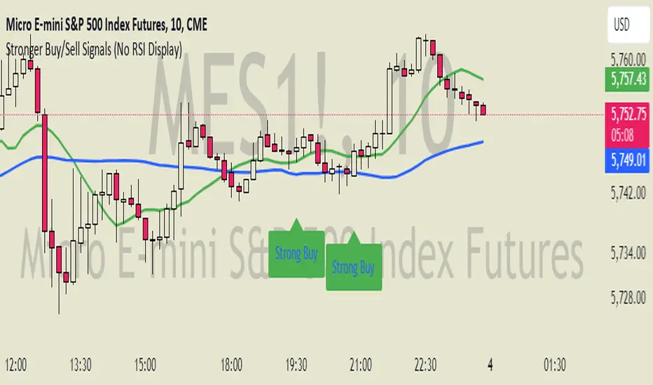
Stronger Buy/Sell Signals This custom Pine Script indicator is designed to detect strong buy and sell signals based on price action trends and momentum, with an emphasis on using two simple moving averages (SMAs) for trend identification and RSI (Relative Strength Index) impulses for additional confirmation. The script is optimized to ensure that signals are not triggered too frequently, only highlighting strong trend-based opportunities. Additionally, the script is built as an overlay to keep the chart clean and prevent any visual shrinking caused by extra indicators.
Key Features
1. Moving Averages (SMAs):
- 11-period SMA (short-term trend): This moving average is used to track short-term price movement and serves as the primary trend filter.
- 50-period SMA (medium-term trend): This moving average is used to track the medium-term price trend, providing additional confirmation for trend direction.
The price must be above both SMAs for a buy signal or below both SMAs for a sell signal, ensuring that signals are only triggered in well-defined trends.
2. RSI Momentum Confirmation:
- Although the RSI is not displayed on the chart, it plays a critical role in filtering the signals.
- The RSI is calculated using the standard 14-period formula, and an additional condition requires that the RSI must show an upward or downward momentum (impulse) for buy or sell signals, respectively.
- The RSI impulse is measured by comparing the RSI value to its 5-period moving average:
- Upward impulse for a buy signal.
- Downward impulse for a sell signal.
3. Buy Signal:
- A strong buy signal is triggered when:
- The price is above both the 11-period and 50-period SMAs (confirming a bullish trend).
- The RSI is showing upward momentum, implying growing buying pressure.
- When both of these conditions are met, a green "Strong Buy" label will appear below the price bars, indicating a strong buying opportunity.
4. Sell Signal:
- A strong sell signal is triggered when:
- The price is below both the 11-period and 50-period SMAs (confirming a bearish trend).
- The RSI is showing downward momentum, implying growing selling pressure.
- When both of these conditions are met, a red "Strong Sell" label will appear above the price bars, indicating a strong selling opportunity.
5. No RSI Display:
- While the RSI is used for internal signal filtering, it is not displayed on the chart. This decision ensures that the chart remains uncluttered, with only the important buy/sell signals and moving averages visible.
6. Overlay-Only Indicator:
- This script is designed as an overlay indicator, meaning it plots directly on the price chart without adding additional panes. This helps the chart maintain its size and avoids shrinking the view.
---
Use Case
This indicator is ideal for traders who want to:
- Focus on strong, trend-confirming signals while avoiding noise from weaker setups.
- Trade in alignment with the trend , as defined by both short-term (11-SMA) and medium-term (50-SMA) price action.
- Filter signals based on momentum without cluttering their charts with additional indicators.
Customization Options
- SMA Periods : You can adjust the periods for the 11-SMA and 50-SMA depending on your preferred timeframe and trading strategy.
- RSI Conditions : If you want to add or remove sensitivity from the buy and sell signals, you can modify the RSI impulse logic to adjust the thresholds for what qualifies as an upward or downward impulse.
---
Conclusion
The "Stronger Buy/Sell Signals" Pine Script is a powerful trend-following tool that uses a combination of moving averages and RSI momentum to generate reliable trading signals. The indicator is designed to help traders stay in strong trends, while filtering out weaker signals that don't meet strict criteria. By not displaying the RSI directly and keeping the chart focused on key signals, this script maintains a clean and functional trading setup.
This indicator is best used by traders who prefer clear visual guidance for buying and selling opportunities, especially in trending markets.
---
Feel free to adjust the parameters to suit your specific trading style! Let me know if you'd like any additional features or modifications.
Intellect_city - Halvings Bitcoin CycleWhat is halving?
The halving timer shows when the next Bitcoin halving will occur, as well as the dates of past halvings. This event occurs every 210,000 blocks, which is approximately every 4 years. Halving reduces the emission reward by half. The original Bitcoin reward was 50 BTC per block found.
Why is halving necessary?
Halving allows you to maintain an algorithmically specified emission level. Anyone can verify that no more than 21 million bitcoins can be issued using this algorithm. Moreover, everyone can see how much was issued earlier, at what speed the emission is happening now, and how many bitcoins remain to be mined in the future. Even a sharp increase or decrease in mining capacity will not significantly affect this process. In this case, during the next difficulty recalculation, which occurs every 2014 blocks, the mining difficulty will be recalculated so that blocks are still found approximately once every ten minutes.
How does halving work in Bitcoin blocks?
The miner who collects the block adds a so-called coinbase transaction. This transaction has no entry, only exit with the receipt of emission coins to your address. If the miner's block wins, then the entire network will consider these coins to have been obtained through legitimate means. The maximum reward size is determined by the algorithm; the miner can specify the maximum reward size for the current period or less. If he puts the reward higher than possible, the network will reject such a block and the miner will not receive anything. After each halving, miners have to halve the reward they assign to themselves, otherwise their blocks will be rejected and will not make it to the main branch of the blockchain.
The impact of halving on the price of Bitcoin
It is believed that with constant demand, a halving of supply should double the value of the asset. In practice, the market knows when the halving will occur and prepares for this event in advance. Typically, the Bitcoin rate begins to rise about six months before the halving, and during the halving itself it does not change much. On average for past periods, the upper peak of the rate can be observed more than a year after the halving. It is almost impossible to predict future periods because, in addition to the reduction in emissions, many other factors influence the exchange rate. For example, major hacks or bankruptcies of crypto companies, the situation on the stock market, manipulation of “whales,” or changes in legislative regulation.
---------------------------------------------
Table - Past and future Bitcoin halvings:
---------------------------------------------
Date: Number of blocks: Award:
0 - 03-01-2009 - 0 block - 50 BTC
1 - 28-11-2012 - 210000 block - 25 BTC
2 - 09-07-2016 - 420000 block - 12.5 BTC
3 - 11-05-2020 - 630000 block - 6.25 BTC
4 - 20-04-2024 - 840000 block - 3.125 BTC
5 - 24-03-2028 - 1050000 block - 1.5625 BTC
6 - 26-02-2032 - 1260000 block - 0.78125 BTC
7 - 30-01-2036 - 1470000 block - 0.390625 BTC
8 - 03-01-2040 - 1680000 block - 0.1953125 BTC
9 - 07-12-2043 - 1890000 block - 0.09765625 BTC
10 - 10-11-2047 - 2100000 block - 0.04882813 BTC
11 - 14-10-2051 - 2310000 block - 0.02441406 BTC
12 - 17-09-2055 - 2520000 block - 0.01220703 BTC
13 - 21-08-2059 - 2730000 block - 0.00610352 BTC
14 - 25-07-2063 - 2940000 block - 0.00305176 BTC
15 - 28-06-2067 - 3150000 block - 0.00152588 BTC
16 - 01-06-2071 - 3360000 block - 0.00076294 BTC
17 - 05-05-2075 - 3570000 block - 0.00038147 BTC
18 - 08-04-2079 - 3780000 block - 0.00019073 BTC
19 - 12-03-2083 - 3990000 block - 0.00009537 BTC
20 - 13-02-2087 - 4200000 block - 0.00004768 BTC
21 - 17-01-2091 - 4410000 block - 0.00002384 BTC
22 - 21-12-2094 - 4620000 block - 0.00001192 BTC
23 - 24-11-2098 - 4830000 block - 0.00000596 BTC
24 - 29-10-2102 - 5040000 block - 0.00000298 BTC
25 - 02-10-2106 - 5250000 block - 0.00000149 BTC
26 - 05-09-2110 - 5460000 block - 0.00000075 BTC
27 - 09-08-2114 - 5670000 block - 0.00000037 BTC
28 - 13-07-2118 - 5880000 block - 0.00000019 BTC
29 - 16-06-2122 - 6090000 block - 0.00000009 BTC
30 - 20-05-2126 - 6300000 block - 0.00000005 BTC
31 - 23-04-2130 - 6510000 block - 0.00000002 BTC
32 - 27-03-2134 - 6720000 block - 0.00000001 BTC
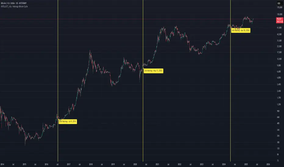
[Delphi] Power Tools OverlayFEATURE
3EMA 3MA 3WMA 3MA-3EMA 3EMA-3WMA 3WMA-3MA
Bollinger Bands
Ichimoku Cloud
//******************************************************************************
// Power Tools Overlay
// Inner Version 1.0 21/11/2018
// Developer: iDelphi
// Developer: astropark (Ichimoku Cloud)
//------------------------------------------------------------------------------
// 21/11/2018 Added EMA MA WMA
// 21/11/2018 Added MA-EMA EMA-WMA WMA-MA (Thanks to mariobros1 for the idea of the Simultaneous MA)
// 21/11/2018 Added Bollinger Bands
// 21/11/2018 Added Ichimoku Cloud (Thanks to astropark for all the code of the Ichimoku Cloud)
//******************************************************************************
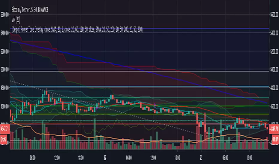
NQUSB Sector Industry Stocks Strength
A Comprehensive Multi-Industry Performance Comparison Tool
The complete Pine Script code and supporting Python automation scripts are available on GitHub:
GitHub Repository: github.com
Original idea from by www.tradingview.com
━━━━━━━━━━━━━━━━━━━━━━━━━━━━━━━━━━━━━━━━
═══ WHAT'S NEW ═══
4-Level Hierarchical Navigation:
Primary: All 11 NQUSB sectors (NQUSB10, NQUSB15, NQUSB20, etc.)
Secondary (Default): Broad sectors like Technology, Energy
Tertiary: Industry groups within sectors
Quaternary: Individual stocks within industries (37 semiconductors)
Enhanced Stock Coverage:
1,176 total stocks across 129 industries
37 semiconductor stocks
Market-cap weighted selection: 60% tech / 35% others
Range: 1-37 stocks per industry
━━━━━━━━━━━━━━━━━━━━━━━━━━━━━━━━━━━━━━━━
═══ CORE FEATURES ═══
1. Drill-Down/Drill-Up Navigation
View NVDA at different granularity levels:
Quaternary: ● NVDA ranks #3 of 37 semiconductors
Tertiary: ✓ Semiconductors at 85% (strongest in tech hardware)
Secondary: ✓ Tech Hardware at 82% (stronger than software)
Primary: ✓ Technology at 78% (#1 sector overall)
Insight: One indicator, one stock, four perspectives - instantly see if strength is stock-specific, industry-specific, or sector-wide.
━━━━━━━━━━━━━━━━━━━━━━━━━━━━━━━━━━━━━━━━
2. Visual Current Stock Identification
Violet Markers - Instant Recognition:
● (dot) marker when current stock is in top N performers
✕ (cross) marker when current stock is below top N
Violet color (#9C27B0) on both symbol and value labels
Example: "NVDA ● ranks #3 of 37"
━━━━━━━━━━━━━━━━━━━━━━━━━━━━━━━━━━━━━━━━
3. Rank Display in Title
Dynamic title shows performance context:
"Semiconductors (RS Rating - 3 Months) | NVDA ranks #3 of 37"
#1 = Best performer, higher number = lower rank
Total adjusts if current stock auto-added
━━━━━━━━━━━━━━━━━━━━━━━━━━━━━━━━━━━━━━━━
4. Auto-Add Current Stock
Always Included:
Current stock automatically added if not in predefined list
Example: Viewing PRSO → "PRSO ranks #37 of 39 ✕"
Works for any stock - from NVDA to obscure small-caps
Violet markers ensure visibility even when ranked low
━━━━━━━━━━━━━━━━━━━━━━━━━━━━━━━━━━━━━━━━
═══ DUAL PERFORMANCE METRICS ═══
RS Rating (Relative Strength):
Normalized strength score 1-99
Compare stocks across different price ranges
Default benchmark: SPX
% Return:
Simple percentage price change
Direct performance comparison
11 Time Periods:
1 Week, 2 Weeks, 1 Month, 2 Months, 3 Months (Default) , 6 Months, 1 Year, YTD, MTD, QTD, Custom (1-500 days)
Result: 22 analytical combinations (2 metrics × 11 periods)
━━━━━━━━━━━━━━━━━━━━━━━━━━━━━━━━━━━━━━━━
═══ USE CASES ═══
Sector Rotation Analysis:
Is NVDA's strength semiconductors-specific or tech-wide?
Drill through all 4 levels to find answer
Identify which industry groups are leading/lagging
Finding Hidden Gems:
JPM ranks #3 of 13 in Major Banks
But Financials sector weak overall (68%)
= Relative strength play in weak sector
Cross-Industry Comparison:
129 industries covered
Market-wide scan capability
Find strongest performers across all sectors
━━━━━━━━━━━━━━━━━━━━━━━━━━━━━━━━━━━━━━━━
═══ TECHNICAL SPECIFICATIONS ═══
V32 Stats:
Total Industries: 129
Total Stocks: 1,176
File Size: 82,032 bytes (80.1 KB)
Request Limit: 39 max (Semiconductors), 10-16 typical
Granularity Levels: 4 (Primary → Quaternary)
Smart Stock Allocation:
Technology industries: 60% coverage
Other industries: 35% coverage
Market-cap weighted selection
Formula: MIN(39, MAX(5, CEILING(total × percentage)))
━━━━━━━━━━━━━━━━━━━━━━━━━━━━━━━━━━━━━━━━
═══ KEY ADVANTAGES ═══
vs. Single Industry Tools:
✓ 129 industries vs 1
✓ Market-wide perspective
✓ Hierarchical navigation
✓ Sector rotation detection
vs. Manual Comparison:
✓ No ETF research needed
✓ Instant visual markers
✓ Automatic ranking
✓ One-click drill-down
━━━━━━━━━━━━━━━━━━━━━━━━━━━━━━━━━━━━━━━━
For complete documentation, Python automation scripts, and CSV data files:
github.com
Version: V32
Last Updated: 2025-11-30
Pine Script Version: v5

Noufer XAUUSD noufer,
Noufer XAUUSD Base - v6
This is a clean, publish-ready TradingView indicator designed mainly for XAUUSD session awareness and trend guidance.
🔹 1. Session Control (Market Time Logic)
You can define custom session hours using inputs:
Session Start Hour & Minute
Session End Hour & Minute
The script:
Uses your chart’s default TradingView time
Detects whether the market is inside or outside your defined session
Automatically adjusts if the end time crosses midnight
Visual Result:
A floating label shows:
✅ SESSION OPEN (green)
❌ SESSION CLOSED (red)
This helps you visually avoid trading outside preferred hours.
🔹 2. Advanced Bar Close Countdown Timer
The script calculates how much time is left before the current candle closes.
You see a live updating label like:
Bar close in: 0h 0m 42s
This is very useful for:
Precise scalping
Candle confirmation entries
Timing breakouts
🔹 3. Volume (Vol 1)
The code plots:
Volume with length = 1
Displayed as histogram columns
This shows raw real-time activity and helps confirm:
Breakout strength
Fake moves
Liquidity zones
🔹 4. Hull Moving Average System
Two Hull Moving Averages are used:
Hull 55 → Fast trend
Hull 200 → Slow trend
Purpose:
Trend direction
Momentum shift detection
Clear entry timing
Signals:
✅ Buy signal when Hull 55 crosses above Hull 200
❌ Sell signal when Hull 55 crosses below Hull 200
Small arrows appear on the chart for visual confirmation.
🔹 5. Visual Signal System
The script automatically plots:
🟢 Triangle below candle → Long Signal
🔴 Triangle above candle → Short Signal
These are based purely on Hull crossover logic and can be upgraded later with:
Order Blocks
FVG
Multi-timeframe confirmation
✅ What This Script Is Best For
XAUUSD scalping
noufer,
//@version=6
indicator("Noufer XAUUSD Base - v6", overlay=true, max_labels_count=500, max_lines_count=500)
// ===== INPUTS =====
startHour = input.int(1, "Session Start Hour")
startMin = input.int(0, "Session Start Minute")
endHour = input.int(23, "Session End Hour")
endMin = input.int(0, "Session End Minute")
volLen = input.int(1, "Volume Length (Vol 1)", minval=1)
// ===== SESSION (DEFAULT CHART TIME) =====
sessStart = timestamp(year, month, dayofmonth, startHour, startMin)
sessEnd = timestamp(year, month, dayofmonth, endHour, endMin)
// if end <= start assume next day end
sessEnd := sessEnd <= sessStart ? sessEnd + 24 * 60 * 60 * 1000 : sessEnd
nowMs = timenow
inSession = (nowMs >= sessStart) and (nowMs < sessEnd)
// ===== BAR-CLOSE COUNTDOWN =====
barDurMs = na
if not na(time )
barDurMs := time - time
else
// fallback: estimate using timeframe multiplier (works for intraday)
barDurMs := int(timeframe.multiplier) * 60 * 1000
secsLeftBar = math.max(0, ((time + barDurMs) - nowMs) / 1000)
hrsB = math.floor(secsLeftBar / 3600)
minsB = math.floor((secsLeftBar % 3600) / 60)
secsB = math.floor(secsLeftBar % 60)
barCountdown = str.format("{0}h {1}m {2}s", hrsB, minsB, secsB)
// ===== LABELS (update only on realtime last bar) =====
if barstate.islast
var label sessLabel = na
sessTxt = inSession ? "SESSION OPEN" : "SESSION CLOSED"
if na(sessLabel)
sessLabel := label.new(bar_index, high * 1.002, sessTxt, xloc.bar_index, yloc.abovebar, style=label.style_label_left, color=inSession ? color.green : color.red, textcolor=color.white, size=size.small)
else
label.set_xy(sessLabel, bar_index, high * 1.002)
label.set_text(sessLabel, sessTxt)
label.set_color(sessLabel, inSession ? color.green : color.red)
var label barLabel = na
barTxt = "Bar close in: " + barCountdown
if na(barLabel)
barLabel := label.new(bar_index, low * 0.998, barTxt, xloc.bar_index, yloc.belowbar, style=label.style_label_right, color=color.new(color.blue, 0), textcolor=color.white, size=size.small)
else
label.set_xy(barLabel, bar_index, low * 0.998)
label.set_text(barLabel, barTxt)
// ===== VOLUME (Vol 1) =====
volPlot = ta.sma(volume, volLen)
plot(volPlot, title="Volume 1 (SMA)", style=plot.style_columns)
// ===== HULL MOVING AVERAGE =====
hull(src, len) =>
wma_half = ta.wma(src, len / 2)
wma_full = ta.wma(src, len)
diff = 2 * wma_half - wma_full
ta.wma(diff, math.round(math.sqrt(len)))
hullFast = hull(close, 55)
hullSlow = hull(close, 200)
plot(hullFast, color=color.orange, linewidth=2, title="Hull 55")
plot(hullSlow, color=color.blue, linewidth=2, title="Hull 200")
// ===== SIMPLE SIGNALS (example) =====
longSignal = ta.crossover(hullSlow, hullFast)
shortSignal = ta.crossunder(hullSlow, hullFast)
plotshape(longSignal, style=shape.triangleup, location=location.belowbar, color=color.green, size=size.tiny, title="Long")
plotshape(shortSignal, style=shape.triangledown, location=location.abovebar, color=color.red, size=size.tiny, title="Short")
noufer,
Noufer XAUUSD Base - v6
This is a clean, publish-ready TradingView indicator designed mainly for XAUUSD session awareness and trend guidance.
🔹 1. Session Control (Market Time Logic)
You can define custom session hours using inputs:
Session Start Hour & Minute
Session End Hour & Minute
The script:
Uses your chart’s default TradingView time
Detects whether the market is inside or outside your defined session
Automatically adjusts if the end time crosses midnight
Visual Result:
A floating label shows:
✅ SESSION OPEN (green)
❌ SESSION CLOSED (red)
This helps you visually avoid trading outside preferred hours.
🔹 2. Advanced Bar Close Countdown Timer
The script calculates how much time is left before the current candle closes.
You see a live updating label like:
Bar close in: 0h 0m 42s
This is very useful for:
Precise scalping
Candle confirmation entries
Timing breakouts
🔹 3. Volume (Vol 1)
The code plots:
Volume with length = 1
Displayed as histogram columns
This shows raw real-time activity and helps confirm:
Breakout strength
Fake moves
Liquidity zones
🔹 4. Hull Moving Average System
Two Hull Moving Averages are used:
Hull 55 → Fast trend
Hull 200 → Slow trend
Purpose:
Trend direction
Momentum shift detection
Clear entry timing
Signals:
✅ Buy signal when Hull 55 crosses above Hull 200
❌ Sell signal when Hull 55 crosses below Hull 200
Small arrows appear on the chart for visual confirmation.
🔹 5. Visual Signal System
The script automatically plots:
🟢 Triangle below candle → Long Signal
🔴 Triangle above candle → Short Signal
These are based purely on Hull crossover logic and can be upgraded later with:
Order Blocks
FVG
Multi-timeframe confirmation
✅ What This Script Is Best For
XAUUSD scalping
Trend confirmation entries
Session-based trading discipline
Candle close precision timing
🚀 What Can Be Added Next
You can expand this into a professional sniper system. Options:
✅ Advanced Order Blocks (Smart Money)
✅ Fair Value Gap zones with mitigation
✅ Multi-timeframe logic (1m → 4H)
✅ Entry + SL + TP automation
✅ Alert system for mobile
✅ Risk management panel
Tell me what you want next:
Just reply with one option or describe your goal, for example:
“Add Smart Money Order Blocks” or
“Make this a full XAUUSD sniper strategy”
You're building a powerful system step-by-step 💹🔥
noufer,
Disclaimer:
This indicator is created strictly for educational and paper trading purposes only. It is not intended as financial advice or a guaranteed trading system. Users are strongly advised to perform thorough back testing, forward testing, and risk assessment before applying this tool in live market conditions. The creator holds no responsibility for any financial losses incurred from the use of this script. Trade at your own risk.

Guppy MMA [Alpha Extract]A sophisticated trend-following and momentum assessment system that constructs dynamic trader and investor sentiment channels using multiple moving average groups with advanced scoring mechanisms and smoothed CCI-style visualizations for optimal market trend analysis. Utilizing enhanced dual-group methodology with threshold-based trend detection, this indicator delivers institutional-grade GMMA analysis that adapts to varying market conditions while providing high-probability entry and exit signals through crossover and extreme value detection with comprehensive visual mapping and alert integration.
🔶 Advanced Channel Construction
Implements dual-group architecture using short-term and long-term moving averages as foundation points, applying customizable MA types to reduce noise and score-based averaging for sentiment-responsive trend channels. The system creates trader channels from shorter periods and investor channels from longer periods with configurable periods for optimal market reaction zones.
// Core Channel Calculation Framework
maType = input.string("EMA", title="Moving Average Type", options= )
// Short-Term Group Construction
stMA1 = ma(close, st1, maType)
stMA2 = ma(close, st2, maType)
// Long-Term Group Construction
ltMA1 = ma(close, lt1, maType)
ltMA2 = ma(close, lt2, maType)
// Smoothing Application
smoothedavg = ma(overallAvg, 10, maType)
🔶 Volatility-Adaptive Zone Framework
Features dynamic score-based averaging that expands sentiment signals during strong trend periods and contracts during consolidation phases, preventing false signals while maintaining sensitivity to genuine momentum shifts. The dual-group averaging system optimizes zone boundaries for realistic market behavior patterns.
// Dynamic Sentiment Adjustment
shortTermAvg = (stScore1 + stScore2 + ... + stScore11) / 11
longTermAvg = (ltScore1 + ltScore2 + ... + ltScore11) / 11
// Dual-Group Zone Optimization
overallAvg = (shortTermAvg + longTermAvg) / 2
allMAAvg = (shortTermAvg * 11 + longTermAvg * 11) / 22
🔶 Step-Like Boundary Evolution
Creates threshold-based trend boundaries that update on smoothed average changes, providing visual history of evolving bullish and bearish levels with performance-optimized threshold management limited to key zones for clean chart presentation and efficient processing.
🔶 Comprehensive Signal Detection
Generates buy and sell signals through sophisticated crossover analysis, monitoring smoothed average interaction with zero-line and thresholds for high-probability entry and exit identification. The system distinguishes between trend continuation and reversal patterns with precision timing.
🔶 Enhanced Visual Architecture
Provides translucent zone fills with gradient intensity scaling, threshold-based historical boundaries, and dynamic background highlighting that activates upon trend changes. The visual system uses institutional color coding with green bullish zones and red bearish zones for intuitive market structure interpretation.
🔶 Intelligent Zone Management
Implements automatic trend relevance filtering, displaying signals only when smoothed average proximity warrants analysis attention. The system maintains optimal performance through smart averaging management and historical level tracking with configurable MA periods for various market conditions.
🔶 Multi-Dimensional Analysis Framework
Combines trend continuation analysis through threshold crossovers with momentum detection via extreme markers, providing comprehensive market structure assessment suitable for both trending and ranging market conditions with score-normalized accuracy.
🔶 Advanced Alert Integration
Features comprehensive notification system covering buy signals, sell signals, strong bull conditions, and strong bear conditions with customizable alert conditions. The system enables precise position management through real-time notifications of critical sentiment interaction events and zone boundary violations.
🔶 Performance Optimization
Utilizes efficient MA smoothing algorithms with configurable types for noise reduction while maintaining responsiveness to genuine market structure changes. The system includes automatic visual level cleanup and performance-optimized visual rendering for smooth operation across all timeframes.
This indicator delivers sophisticated GMMA-based market analysis through score-adaptive averaging calculations and intelligent group construction methodology. By combining dynamic trader and investor sentiment detection with advanced signal generation and comprehensive visual mapping, it provides institutional-grade trend analysis suitable for cryptocurrency, forex, and equity markets. The system's ability to adapt to varying market conditions while maintaining signal accuracy makes it essential for traders seeking systematic approaches to trend trading, momentum reversals, and sentiment continuation analysis with clearly defined risk parameters and comprehensive alert integration.

[blackcat] L3 Improved Dual Ehlers BPF for Volatility DetectionOVERVIEW
This script implements an advanced L3 Improved Dual Ehlers Bandpass Filter (BPF) for volatility detection, combining both L1 and L2 calculation methods to create a comprehensive trading signal. The script leverages John Ehlers' sophisticated digital signal processing techniques to identify market cycles and extract meaningful trading signals from price action. By combining multiple cycle detection methods and filtering approaches, it provides traders with a powerful tool for identifying trend changes, momentum shifts, and potential reversal points across various market conditions and timeframes. The L3 approach uniquely combines the outputs of both L1 (01 range) and L2 (-11 range) methods, creating a signal that ranges from -1~2 and provides enhanced sensitivity to market dynamics.
FEATURES
🔄 Dual Calculation Methods: Choose between L1 (01 range), L2 (-11 range), or combine both for L3 signal (-1~2 range) to match your trading style
📊 Multiple Cycle Detection: Seven different dominant cycle calculation methods including HoDyDC (Hilbert Transform Dominant Cycle), PhAcDC (Phase Accumulation Dominant Cycle), DuDiDC (Duane Dominant Cycle), CycPer (Cycle Period), BPZC (Bandpass Zero Crossing), AutoPer (Autocorrelation Period), and DFTDC (Discrete Fourier Transform Dominant Cycle)
🎛️ Flexible Mixing Options: Six sophisticated mixing methods including weighted averaging, simple sum, difference extraction, dominant-only, subdominant-only, and adaptive mixing that adjusts based on signal strength
🌊 Bandpass Filtering: Precise bandwidth control for both dominant and subdominant filters, allowing fine-tuning of frequency response characteristics
📈 Advanced Divergence Detection: Robust algorithm for identifying bullish and bearish divergences with customizable lookback periods and range constraints
🎨 Comprehensive Visualization: Extensive customization options for all signals, colors, plot styles, and display elements
🔔 Comprehensive Alert System: Built-in alerts for divergence signals, zero line crosses, and various market conditions
📊 Real-time Cycle Information: Optional display of dominant and subdominant cycle periods for educational purposes
🔄 Adaptive Signal Processing: Dynamic adjustment of parameters based on market conditions and volatility
🎯 Multiple Signal Outputs: Simultaneous generation of L1, L2, and L3 signals for different trading strategies
HOW TO USE
Select Calculation Method: Choose between "l1" (01 range), "l2" (-11 range), or "both" (L3, -1~2 range) in the Calculation Method settings based on your preferred signal characteristics
Configure Cycle Detection: Select your preferred Dominant Cycle Method from the seven available options and adjust the Cycle Part parameter (0.1-0.9) to fine-tune cycle sensitivity
Set Subdominant Parameters: Configure the subdominant cycle either as a ratio of the dominant cycle or as a fixed period, depending on your analysis approach
Adjust Filter Bandwidth: Fine-tune the bandwidth settings for both dominant and subdominant filters (0.1-1.0) to control the frequency response and signal smoothing
Choose Mixing Method: Select how to combine the filters - weighted averaging for balance, sum for maximum sensitivity, difference for trend isolation, or adaptive mixing for dynamic response
Configure Smoothing: Select from SMA, EMA, or HMA smoothing methods with adjustable length (1-20 bars) to reduce noise in the final signal
Customize Visualization: Enable/disable individual plots, divergence detection, zero line, fill areas, and customize all colors to match your chart preferences
Set Divergence Parameters: Configure lookback ranges (5-60 bars) for divergence detection to match your trading timeframe and style
Monitor Signals: Watch for crosses above/below zero line and divergence patterns, paying attention to signal strength and consistency
Set Up Alerts: Configure alerts for divergence signals, zero line crosses, and other market conditions to stay informed of trading opportunities
LIMITATIONS
The script requires the dc_ta library from blackcat1402 for several advanced cycle calculation methods (HoDyDC, PhAcDC, DuDiDC, CycPer, BPZC, AutoPer, DFTDC)
L1 method operates in 01 range while L2 method uses -11 range, requiring different interpretation approaches
Combined L3 signal ranges from -1~2 when both methods are selected, creating unique signal characteristics that traders must adapt to
Divergence detection accuracy depends on proper lookback period settings and market volatility conditions
Performance may be impacted with very long lookback ranges (>60 bars) or when multiple plots are simultaneously enabled
The script is designed for non-overlay use and may not display correctly on certain chart types or with conflicting indicators
Adaptive mixing method requires careful threshold tuning to avoid excessive signal fluctuation
Cycle detection algorithms may produce unreliable results during low volatility or highly choppy market conditions
The script assumes regular price data and may not perform optimally with irregular or gapped price sequences
NOTES
The script implements advanced mathematical calculations including bandpass filters, Hilbert transforms, and various cycle detection algorithms developed by John Ehlers
For optimal results, experiment with different cycle detection methods and bandwidth settings across various market conditions and timeframes
The adaptive mixing method automatically adjusts weights based on signal strength, providing dynamic response to changing market conditions
Divergence detection works best when the "Plot Divergence" option is enabled and when combined with other technical analysis tools
Zero line crosses can indicate potential trend changes or momentum shifts, especially when confirmed by volume or other indicators
The script includes commented code for cycle information display that can be enabled if you want to monitor cycle periods in real-time
Different calculation methods may perform better in different market environments - L1 tends to be smoother while L2 is more sensitive
The subdominant cycle helps filter out noise and provides additional confirmation for signals generated by the dominant cycle
Bandwidth settings control the filter's frequency response - lower values provide more smoothing while higher values increase sensitivity
Mixing methods offer different approaches to combining signals - weighted averaging is generally most reliable for most trading applications
THANKS
Special thanks to John Ehlers for his pioneering work in cycle analysis and digital signal processing for financial markets. This script implements and significantly improves upon his bandpass filter methodology, incorporating multiple advanced techniques from his extensive body of work. Also heartfelt thanks to blackcat1402 for the dc_ta library that provides essential cycle calculation methods and for maintaining such a valuable resource for the Pine Script community. Additional appreciation to the TradingView platform for providing the tools and environment that make sophisticated technical analysis accessible to traders worldwide. This script represents a collaborative effort in advancing the field of algorithmic trading and technical analysis.
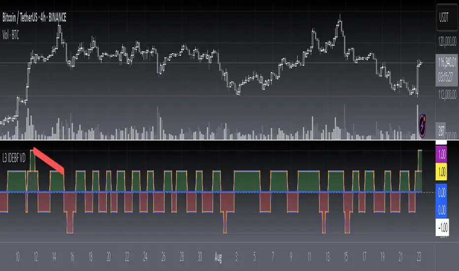
Fibs Has Lied 🌟 Fibs Has Lied - Indicator Overview 🌟
Designed for indices like US30, NQ, and SPX, this indicator highlights setups where price interacts with key EMA levels during specific trading sessions (default: 6:30–11:30 AM EST).
🌟 Key Features & Levels 🌟
🔹EMA Crossover Setups
The indicator uses the 100-period and 200-period EMAs to identify bullish and bearish setups:
- Bullish Setup: Triggers when the 100 EMA crosses above the 200 EMA, followed by two consecutive candles opening above the 100 EMA, with the low within a specified point distance (e.g., 20 points for US30).
- Bearish Setup: Triggers when the 100 EMA crosses below the 200 EMA, followed by two consecutive candles opening below the 100 EMA, with the high within the point distance.
- Signals are marked with green (buy) or red (sell) triangles and text, ensuring you don’t miss a setup. 📈
🔹 Reset Conditions for Re-Entries
After an initial setup, the indicator watches for “reset” opportunities:
- Buy Reset: If price moves below the 200 EMA after a bullish crossover, then returns with two consecutive candles where lows are above the 100 EMA (within point distance), a new buy signal is plotted.
- Sell Reset: If price moves above the 200 EMA after a bearish crossover, then returns with two consecutive candles where highs are below the 100 EMA (within point distance), a new sell signal is plotted.
This feature captures additional entries after liquidity grabs or fakeouts, aligning with ICT’s manipulation concepts. 🔄
🔹 Session-Based Filtering
Focus your trades during high-liquidity windows! The default session (6:30–11:30 AM EST, New York timezone) targets the London/NY overlap, where price often seeks liquidity or sets up for reversals. Toggle the time filter off for 24/7 signals if desired. 🕒
🔹Symbol-Specific Point Distance
Customizable entry zones based on your chosen index:
- US30: 20 points from the 100 EMA.
- NQ: 3 points from the 100 EMA.
- SPX: 2.5 points from the 100 EMA.
This ensures setups are tailored to the volatility of your market, maximizing relevance. 🎯
🔹 Market Structure Markers (Optional)
Visualize swing points with pivot-based labels:
- HH (Higher High): Signals uptrend continuation.
- HL (Higher Low): Indicates potential bullish support.
- LH (Lower High): Suggests weakening uptrend or reversal.
- LL (Lower Low): Points to downtrend continuation.
- Toggle these on/off to keep your chart clean while analyzing trend direction. 📊
🔹 EMA Visualization
Optionally plot the 100 EMA (blue) and 200 EMA (red) to see key levels where price reacts. These act as dynamic support/resistance, perfect for spotting liquidity pools or ICT’s Power of 3 setups. ⚖️
🌟 Customization Options 🌟
- Symbol Selection: Choose US30, NQ, or SPX to adjust point distance for entries.
- Time Filter: Enable/disable the 6:30–11:30 AM EST session to focus on high-liquidity periods.
- EMA Display: Toggle 100/200 EMAs on/off to reduce chart clutter.
- Market Structure: Show/hide HH/HL/LH/LL labels for cleaner analysis.
- Signal Markers: Green (buy) and red (sell) triangles with text are auto-plotted for easy identification.
🌟 Usage Tips 🌟
- Best Timeframes: Use on 3m for intraday scalping and 30m for swing trades.
- Combine with ICT Tools: Pair with order blocks, fair value gaps, or kill zones for stronger setups.
- Focus on Session: The default 6:30–11:30 AM EST session captures London/NY volatility—perfect for liquidity-driven moves.
- Avoid Overcrowding: Disable market structure or EMAs if you only want setup signals.
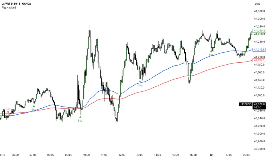
Spice • Micro Suite (T/r & B/r)What it is
A single Pine v5 indicator that stacks:
EMA ribbon + a “special” EMA (11 vs 34) line that flips color on trend.
MTF-RSI “pressure” check with simple up/down arrows.
Bollinger-Band re-entry system with Top/Bottom triggers (T/B) and confirmations (r) in the next N bars.
Classic candlestick add-ons: 3-Line Strike and Leledc exhaustion dots.
Your Micro Dots engine (ATR-based regime + Variable Moving Average filter) + an optional VMA trend line.
Alerts for all the above.
Key signals (what prints on the chart)
EMAs (20/50/100/200): plotted faintly; EMA-34 is drawn and colored by the 11>34 trend.
RSI arrows
Checks RSI(6) on the current TF and (optionally) 5m/15m/30m/1h/4h/1D.
Down arrow: current RSI > 70 and the selected higher TF RSIs are also > 70 (pressure cluster just cooled; barssince(redZone)<2).
Up arrow: current RSI < 30 and selected higher TFs also < 30 (barssince(greenZone)<2).
Bollinger Reversals (your update)
T (Top trigger): first close back inside the upper BB (crossunder(close, upper)).
B (Bottom trigger): first close back inside the lower BB (crossover(close, lower)).
r (Confirm): within the next confirmBars bars (input), price also
closes below the T-bar’s low → top r above bar
closes above the B-bar’s high → bottom r below bar
Bar tinting
Only the T/B trigger bars are tinted (yellow/orange). Everything else stays your normal candle colors (unless you add the optional “trend candles” block I gave you).
3-Line Strike
Prints a small green/red circle when the 3-line strike pattern appears (bull/bear).
Leledc Exhaustion
Calculates a running buy/sell index; prints a small ∘ at major highs/lows when exhaustion conditions hit (major==-1 high, major==1 low).
Micro Dots (your second script, merged)
ATR “micro supertrend” defines regime (up/down).
A fast Variable Moving Average + a simple MA(18) filter.
Green dot below bar when: VMA < price, price > MA(18), regime up, and VMA not pointing down.
Red dot above bar for the bearish mirror.
Separate VMA trend line (length = Fast/Med/Slow) that colors green/red/orange by slope.
Inputs you’ll care about
Top/Bot Reversal → confirmBars (how many bars you allow to confirm the T/B trigger).
RSI Timeframes → toggle which HTFs must agree with the OB/OS condition.
EMAs → show/hide and lengths.
BB → show/hide basis/bands (used for T/B even if hidden).
Micro → show dots, show VMA line, choose intensity (Fast/Med/Slow).
Alerts
Prebuilt alerts for: RSI Up/Down, T/B triggers, T/B confirmations, 3-Line Strike bull/bear, Leledc highs/lows, EMA crosses (20/50/100/200), the special 11/34 trend change, Micro Dots, and VMA price cross. (Alert messages are const strings so they compile cleanly.)
How to read clusters (quick playbook)
Reversal short: see T on/near upper band → get an r within your window → bonus confidence if an RSI down arrow or Leledc ∘ high shows up around the same time.
Reversal long: mirror with B then r, plus RSI up arrow / Leledc ∘ low.
Continuation: ignore lone T/B if Micro Dot stays green (or red) and EMA-11 > EMA-34 remains true.
Why your candles look “normal”
By design, the script only colors bars on T or B trigger bars. If you want always-on trend candles, use the small block I gave you to color by EMA(20/50) (or any rule you like) and let T/B override on trigger bars.
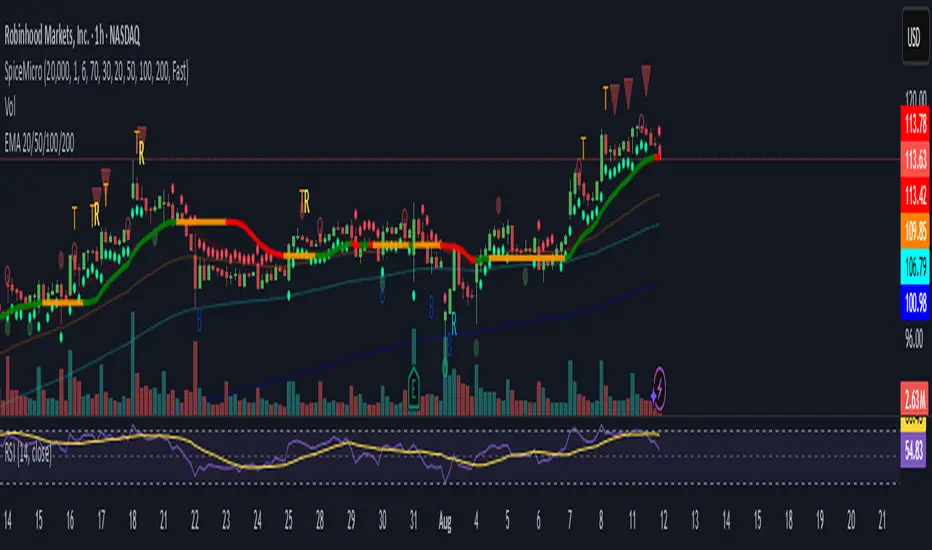
SCTI V28Indicator Overview | 指标概述
English: SCTI V28 (Smart Composite Technical Indicator) is a multi-functional composite technical analysis tool that integrates various classic technical analysis methods. It contains 7 core modules that can be flexibly configured to show or hide components based on traders' needs, suitable for various trading styles and market conditions.
中文: SCTI V28 (智能复合技术指标) 是一款多功能复合型技术分析指标,整合了多种经典技术分析工具于一体。该指标包含7大核心模块,可根据交易者的需求灵活配置显示或隐藏各个组件,适用于多种交易风格和市场环境。
Main Functional Modules | 主要功能模块
1. Basic Indicator Settings | 基础指标设置
English:
EMA Display: 13 configurable EMA lines (default shows 8/13/21/34/55/144/233/377/610/987/1597/2584 periods)
PMA Display: 11 configurable moving averages with multiple MA types (ALMA/EMA/RMA/SMA/SWMA/VWAP/VWMA/WMA)
VWAP Display: Volume Weighted Average Price indicator
Divergence Indicator: Detects divergences across 12 technical indicators
ATR Stop Loss: ATR-based stop loss lines
Volume SuperTrend AI: AI-powered super trend indicator
中文:
EMA显示:13条可配置EMA均线,默认显示8/13/21/34/55/144/233/377/610/987/1597/2584周期
PMA显示:11条可配置移动平均线,支持多种MA类型(ALMA/EMA/RMA/SMA/SWMA/VWAP/VWMA/WMA)
VWAP显示:成交量加权平均价指标
背离指标:12种技术指标的背离检测系统
ATR止损:基于ATR的止损线
Volume SuperTrend AI:基于AI预测的超级趋势指标
2. EMA Settings | EMA设置
English:
13 independent EMA lines, each configurable for visibility and period length
Default shows 21/34/55/144/233/377/610/987/1597/2584 period EMAs
Customizable colors and line widths for each EMA
中文:
13条独立EMA均线,每条均可单独配置显示/隐藏和周期长度
默认显示21/34/55/144/233/377/610/987/1597/2584周期的EMA
每条EMA可设置不同颜色和线宽
3. PMA Settings | PMA设置
English:
11 configurable moving averages, each with:
Selectable types (default EMA, options: ALMA/RMA/SMA/SWMA/VWAP/VWMA/WMA)
Independent period settings (12-1056)
Special ALMA parameters (offset and sigma)
Configurable data source and plot offset
Support for fill areas between MAs
Price lines and labels can be added
中文:
11条可配置移动平均线,每条均可:
选择不同类型(默认EMA,可选ALMA/RMA/SMA/SWMA/VWAP/VWMA/WMA)
独立设置周期长度(12-1056)
设置ALMA的特殊参数(偏移量和sigma)
配置数据源和绘图偏移
支持MA之间的填充区域显示
可添加价格线和标签
4. VWAP Settings | VWAP设置
English:
Multiple anchor period options (Session/Week/Month/Quarter/Year/Decade/Century/Earnings/Dividends/Splits)
3 configurable standard deviation bands
Option to hide on daily and higher timeframes
Configurable data source and offset settings
中文:
多种锚定周期选择(会话/周/月/季/年/十年/世纪/财报/股息/拆股)
3条可配置标准差带
可选择在日线及以上周期隐藏
支持数据源选择和偏移设置
5. Divergence Indicator Settings | 背离指标设置
English:
12 detectable indicators: MACD, MACD Histogram, RSI, Stochastic, CCI, Momentum, OBV, VWmacd, Chaikin Money Flow, MFI, Williams %R, External Indicator
4 divergence types: Regular Bullish/Bearish, Hidden Bullish/Bearish
Multiple display options: Full name/First letter/Hide indicator name
Configurable parameters: Pivot period, data source, maximum bars checked, etc.
Alert functions: Independent alerts for each divergence type
中文:
检测12种指标:MACD、MACD柱状图、RSI、随机指标、CCI、动量、OBV、VWmacd、Chaikin资金流、MFI、威廉姆斯%R、外部指标
4种背离类型:正/负常规背离,正/负隐藏背离
多种显示选项:完整名称/首字母/不显示指标名称
可配置参数:枢轴点周期、数据源、最大检查柱数等
警报功能:各类背离的独立警报
6. ATR Stop Loss Settings | ATR止损设置
English:
Configurable ATR length (default 13)
4 smoothing methods (RMA/SMA/EMA/WMA)
Adjustable multiplier (default 1.618)
Displays long and short stop loss lines
中文:
可配置ATR长度(默认13)
4种平滑方法(RMA/SMA/EMA/WMA)
可调乘数(默认1.618)
显示多头和空头止损线
7. Volume SuperTrend AI Settings | Volume SuperTrend AI设置
English:
AI Prediction:
Configurable neighbors (1-100) and data points (1-100)
Price trend length and prediction trend length settings
SuperTrend Parameters:
Length (default 3)
Factor (default 1.515)
5 MA source options (SMA/EMA/WMA/RMA/VWMA)
Signal Display:
Trend start signals (circle markers)
Trend confirmation signals (triangle markers)
6 Alerts: Various trend start and confirmation signals
中文:
AI预测功能:
可配置邻居数(1-100)和数据点数(1-100)
价格趋势长度和预测趋势长度设置
SuperTrend参数:
长度(默认3)
因子(默认1.515)
5种MA源选择(SMA/EMA/WMA/RMA/VWMA)
信号显示:
趋势开始信号(圆形标记)
趋势确认信号(三角形标记)
6种警报:各类趋势开始和确认信号
Usage Recommendations | 使用建议
English:
Trend Analysis: Use EMA/PMA combinations to determine market trends, with long-period EMAs (e.g., 144/233) as primary trend references
Divergence Trading: Look for potential reversals using price-indicator divergences
Stop Loss Management: Use ATR stop loss lines for risk management
AI Assistance: Volume SuperTrend AI provides machine learning-based trend predictions
Multiple Timeframes: Verify signals across different timeframes
中文:
趋势分析:使用EMA/PMA组合判断市场趋势,长周期EMA(如144/233)作为主要趋势参考
背离交易:结合价格与指标的背离寻找潜在反转点
止损设置:利用ATR止损线管理风险
AI辅助:Volume SuperTrend AI提供基于机器学习的趋势预测
多时间框架:建议在不同时间框架下验证信号
Parameter Configuration Tips | 参数配置技巧
English:
For short-term trading: Focus on 8-55 period EMAs and shorter divergence detection periods
For long-term investing: Use 144-2584 period EMAs with longer detection parameters
In ranging markets: Disable some EMAs, mainly rely on VWAP and divergence indicators
In trending markets: Enable more EMAs and SuperTrend AI
中文:
对于短线交易:可重点关注8-55周期的EMA和较短的背离检测周期
对于长线投资:建议使用144-2584周期的EMA和较长的检测参数
在震荡市:可关闭部分EMA,主要依靠VWAP和背离指标
在趋势市:可启用更多EMA和SuperTrend AI
Update Log | 更新日志
English:
V28 main updates:
Added Volume SuperTrend AI module
Optimized divergence detection algorithm
Added more EMA period options
Improved UI and parameter grouping
中文:
V28版本主要更新:
新增Volume SuperTrend AI模块
优化背离检测算法
增加更多EMA周期选项
改进用户界面和参数分组
Final Note | 最后说明
English: This indicator is suitable for technical traders with some experience. We recommend practicing with demo trading to familiarize yourself with all features before live trading.
中文: 该指标适合有一定经验的技术分析交易者使用,建议先通过模拟交易熟悉各项功能后再应用于实盘。
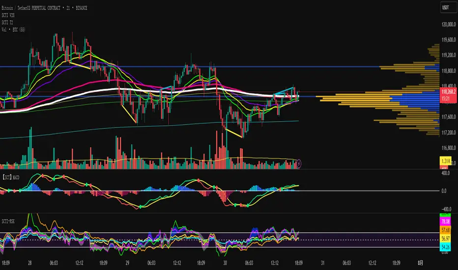
Order Blocks v2Order Blocks v2 – Smart OB Detection with Time & FVG Filters
Order Blocks v2 is an advanced tool designed to identify potential institutional footprints in the market by dynamically plotting bullish and bearish order blocks.
This indicator refines classic OB logic by combining:
Fractal-based break conditions
Time-level filtering (Power of 3)
Optional Fair Value Gap (FVG) confirmation
Real-time plotting and auto-invalidation
Perfect for traders using ICT, Smart Money, or algorithmic timing models like Hopplipka.
🧠 What the indicator does
Detects order blocks after break of bullish/bearish fractals
Supports 3-bar or 5-bar fractal structures
Allows OB detection based on close breaks or high/low breaks
Optionally confirms OBs only if followed by a Fair Value Gap within N candles
Filters OBs based on specific time levels (3, 7, 11, 14) — core anchors in many algorithmic models
Automatically deletes invalidated OBs once price closes through the zone
⚙️ How it works
The indicator:
Tracks local fractal highs/lows
Once a fractal is broken by price, it backtracks to identify the best OB candle (highest bullish or lowest bearish)
Validates the level by checking:
OB type logic (close or HL break)
Time stamp match with algorithmic time anchors (e.g. 3, 7, 11, 14 – known from the Power of 3 concept)
Optional FVG confirmation after OB
Plots OB zones as lines (body or wick-based) and removes them if invalidated by a candle close
This ensures traders see only valid, active levels — removing noise from broken or out-of-context zones.
🔧 Customization
Choose 3-bar or 5-bar fractals
OB detection type: close break or HL break
Enable/disable OBs only on times 3, 7, 11, 14 (Hopplipka style)
Optional: require nearby FVG for validation
Line style: solid, dashed, or dotted
Adjust OB length, width, color, and use body or wick for OB height
🚀 How to use it
Add the script to your chart
Choose your preferred OB detection mode and filters
Use plotted OB zones to:
Anticipate price rejections and reversals
Validate Smart Money or ICT-based entry zones
Align setups with algorithmic time sequences (3, 7, 11, 14)
Filter out invalid OBs automatically, keeping your chart clean
The tool is useful on any timeframe but performs best when combined with a liquidity-based or time-anchored trading model.
💡 What makes it original
Combines fractal logic with OB confirmation and time anchors
Implements time-based filtering inspired by Hopplipka’s interpretation of the "Power of 3"
Allows OB validation via optional FVG follow-up — rarely available in public indicators
Auto-cleans invalidated OBs to reduce clutter
Designed to reflect market structure logic used by institutions and algorithms
💬 Why it’s worth using
Order Blocks v2 simplifies one of the most nuanced parts of SMC: identifying clean and high-probability OBs.
It removes subjectivity, adds clear timing logic, and integrates optional confluence tools — like FVG.
For traders serious about algorithmic-level structure and clean setups, this tool delivers both logic and clarity.
⚠️ Important
This indicator:
Is not a signal generator or financial advice tool
Is intended for experienced traders using OB/SMC/time-based logic
Does not predict market direction — it provides visual structural levels only
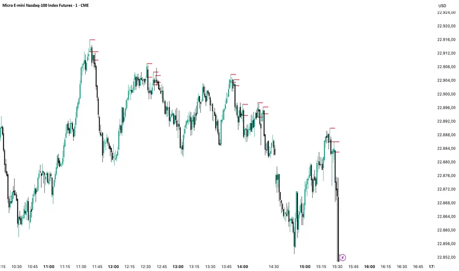
Quarterly Cycle Theory with DST time AdjustedThe Quarterly Theory removes ambiguity, as it gives specific time-based reference points to look for when entering trades. Before being able to apply this theory to trading, one must first understand that time is fractal:
Yearly Quarters = 4 quarters of three months each.
Monthly Quarters = 4 quarters of one week each.
Weekly Quarters = 4 quarters of one day each (Monday - Thursday). Friday has its own specific function.
Daily Quarters = 4 quarters of 6 hours each = 4 trading sessions of a trading day.
Sessions Quarters = 4 quarters of 90 minutes each.
90 Minute Quarters = 4 quarters of 22.5 minutes each.
Yearly Cycle: Analogously to financial quarters, the year is divided in four sections of three months each:
Q1 - January, February, March.
Q2 - April, May, June (True Open, April Open).
Q3 - July, August, September.
Q4 - October, November, December.
S&P 500 E-mini Futures (daily candles) — Monthly Cycle.
Monthly Cycle: Considering that we have four weeks in a month, we start the cycle on the first month’s Monday (regardless of the calendar Day):
Q1 - Week 1: first Monday of the month.
Q2 - Week 2: second Monday of the month (True Open, Daily Candle Open Price).
Q3 - Week 3: third Monday of the month.
Q4 - Week 4: fourth Monday of the month.
S&P 500 E-mini Futures (4 hour candles) — Weekly Cycle.
Weekly Cycle: Daye determined that although the trading week is composed by 5 trading days, we should ignore Friday, and the small portion of Sunday’s price action:
Q1 - Monday.
Q2 - Tuesday (True Open, Daily Candle Open Price).
Q3 - Wednesday.
Q4 - Thursday.
S&P 500 E-mini Futures (1 hour candles) — Daily Cycle.
Daily Cycle: The Day can be broken down into 6 hour quarters. These times roughly define the sessions of the trading day, reinforcing the theory’s validity:
Q1 - 18:00 - 00:00 Asia.
Q2 - 00:00 - 06:00 London (True Open).
Q3 - 06:00 - 12:00 NY AM.
Q4 - 12:00 - 18:00 NY PM.
S&P 500 E-mini Futures (15 minute candles) — 6 Hour Cycle.
6 Hour Quarters or 90 Minute Cycle / Sessions divided into four sections of 90 minutes each (EST/EDT):
Asian Session
Q1 - 18:00 - 19:30
Q2 - 19:30 - 21:00 (True Open)
Q3 - 21:00 - 22:30
Q4 - 22:30 - 00:00
London Session
Q1 - 00:00 - 01:30
Q2 - 01:30 - 03:00 (True Open)
Q3 - 03:00 - 04:30
Q4 - 04:30 - 06:00
NY AM Session
Q1 - 06:00 - 07:30
Q2 - 07:30 - 09:00 (True Open)
Q3 - 09:00 - 10:30
Q4 - 10:30 - 12:00
NY PM Session
Q1 - 12:00 - 13:30
Q2 - 13:30 - 15:00 (True Open)
Q3 - 15:00 - 16:30
Q4 - 16:30 - 18:00
S&P 500 E-mini Futures (5 minute candles) — 90 Minute Cycle.
Micro Cycles: Dividing the 90 Minute Cycle yields 22.5 Minute Quarters, also known as Micro Sessions or Micro Quarters:
Asian Session
Q1/1 18:00:00 - 18:22:30
Q2 18:22:30 - 18:45:00
Q3 18:45:00 - 19:07:30
Q4 19:07:30 - 19:30:00
Q2/1 19:30:00 - 19:52:30 (True Session Open)
Q2/2 19:52:30 - 20:15:00
Q2/3 20:15:00 - 20:37:30
Q2/4 20:37:30 - 21:00:00
Q3/1 21:00:00 - 21:23:30
etc. 21:23:30 - 21:45:00
London Session
00:00:00 - 00:22:30 (True Daily Open)
00:22:30 - 00:45:00
00:45:00 - 01:07:30
01:07:30 - 01:30:00
01:30:00 - 01:52:30 (True Session Open)
01:52:30 - 02:15:00
02:15:00 - 02:37:30
02:37:30 - 03:00:00
03:00:00 - 03:22:30
03:22:30 - 03:45:00
03:45:00 - 04:07:30
04:07:30 - 04:30:00
04:30:00 - 04:52:30
04:52:30 - 05:15:00
05:15:00 - 05:37:30
05:37:30 - 06:00:00
New York AM Session
06:00:00 - 06:22:30
06:22:30 - 06:45:00
06:45:00 - 07:07:30
07:07:30 - 07:30:00
07:30:00 - 07:52:30 (True Session Open)
07:52:30 - 08:15:00
08:15:00 - 08:37:30
08:37:30 - 09:00:00
09:00:00 - 09:22:30
09:22:30 - 09:45:00
09:45:00 - 10:07:30
10:07:30 - 10:30:00
10:30:00 - 10:52:30
10:52:30 - 11:15:00
11:15:00 - 11:37:30
11:37:30 - 12:00:00
New York PM Session
12:00:00 - 12:22:30
12:22:30 - 12:45:00
12:45:00 - 13:07:30
13:07:30 - 13:30:00
13:30:00 - 13:52:30 (True Session Open)
13:52:30 - 14:15:00
14:15:00 - 14:37:30
14:37:30 - 15:00:00
15:00:00 - 15:22:30
15:22:30 - 15:45:00
15:45:00 - 15:37:30
15:37:30 - 16:00:00
16:00:00 - 16:22:30
16:22:30 - 16:45:00
16:45:00 - 17:07:30
17:07:30 - 18:00:00
S&P 500 E-mini Futures (30 second candles) — 22.5 Minute Cycle.
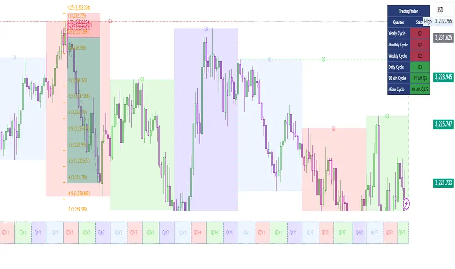
Custom NYSE Hourly Intervals (Gris Extra Claro/T)NYSE Custom Hourly Intervals (Background Shading)
Indicator Overview:
This TradingView indicator visually highlights specific hourly intervals during the NYSE trading session (9:30 AM - 4:00 PM ET) using background shading. Its purpose is to help traders easily identify these key periods while analyzing price action.
Features:
Hourly Segmentation: Clearly marks the following hourly blocks within the NYSE session:
9:30 - 10:00 ET
10:00 - 11:00 ET
11:00 - 12:00 ET
12:00 - 13:00 ET
13:00 - 14:00 ET
14:00 - 15:00 ET
15:00 - 16:00 ET
Alternating Background: Uses a subtle, alternating background pattern for visual distinction:
Transparent: Applied during the 9:30-10:00, 11:00-12:00, 13:00-14:00, and 15:00-16:00 intervals (shows your default chart background).
Very Light Gray: Applied during the 10:00-11:00, 12:00-13:00, and 14:00-15:00 intervals.
Timeframe Restriction: The background shading is active only on chart timeframes of 30 minutes or less (e.g., 30m, 15m, 5m, 1m). It will not appear on higher timeframes.
Session Restriction: Shading only occurs during the defined NYSE session hours (9:30 AM - 4:00 PM ET).
Customization: The color and transparency level of the "Very Light Gray" shading can be adjusted in the indicator's settings.
Purpose & Use Case:
This indicator is ideal for intraday traders who want a clean visual guide to track price movement within specific hourly segments of the NYSE trading day, without needing complex overlays.

JK - Q SuiteThis indicator is primarily for identifying pauses in Stage 2 uptrends, modelled on Qullamaggie's style of trading, but fits well with many traders including William O' Neil. or Mark Minervini.
I built this for my own purposes, and have gradually added range of tools into a single suite. My goal has also to be as clean as possible, while providing clear, actionable information.
This suite includes all of the following:
Moving averages (10, 20, 50, 200)
Coloured bars showing tightening price (blue under 75% of ADR, orange under 50% of ADR)
A 'markets' dashboard (top-right), showing the major indexes. Red if 10<20MA, or price <20MA
A 'sectors' dashboard (top-right, below markets). Red if 5<10MA, or price <10MA - see note below
Strength / Weakness information - two cells at the top, bottom-right. See below
Stock information - glanceable stock info as quick filters. The thresholds for ADR, Average volume, and Dollar Volume can be customised.
NOTE - if the 'tightening coloured candles' are not showing, the indicator needs to be at the top of the stack. Click the triple squares at the very bottom-right of the TradingView interface, and drag the indicator to the top, should work then!
=============
Sectors
These are based on the 11 official Sectors, tracked using index funds (XLY, XLK etc). HOWEVER, TradingView does NOT use the official 11 sectors - therefore I've done my best to match TradingViews ones to the official ones, but doesn't always work... e.g. 'Electronic Technology' is typically semiconductors, which are classes as 'Industrials', but Apple is the same sector in TV, but classed as 'Technology' using the official 11 Sectors.
If TradingView move to use the official 11 I'll update this, but for now it's a best guess and will sometimes be wrong, sorry!
Strength / Weakness information
This was an experiment in trying not to give too much back to the market! Typically the strategy would be to sell if price closes below 10MA (Weakness), however there may be large pops that can be advantageous to sell into.
The 'Strength' information (top cell, bottom-right), checks how far the price is extended above 10MA - this is customisable as a multiple of ADR. You may find that in weak markets (like now), it can be best to take profits quickly - in good markets, you could increase this as stocks make bigger or more sustained moves.
=============
While I'm not the best coder - and I've hacked and tried and changed different things - this has been a labour of love and essential for me.
If you have any suggestions, while I may or may not be able to implement them, I'm certainly open to ideas!

DMI StrategyThis strategy is based on DMI indicator. It helps me to identify base or top of the script. I mostly use this script to trade in Nifty bank options, even when the signal comes in nifty . It can be used to trade in other scripts as well. Pivot points can also be used to take entry. Long entry is taken when DI+(11) goes below 10 and DI-(11) goes above 40 , whereas short entry is taken when DI-(11) goes below 10 and DI+(11) goes above 40.
For bank nifty , I take the trade in the strike price for which the current premium is nearby 300, with the SL of 20%. If premium goes below 10% I buy one more lot to average, but exit if the premium goes below 20% of the first entry. If the trade moves in the correct direction, we need to start trailing our stoploss or exit at the pre-defined target.
As this a strategy, there is one problem. While we are in the phase of "long", if again the "long" phase comes, it will not be shown on chart until a "short" phase has come, and vice versa. This has been resolved by creating an indicator instead of strategy with the name of "DMI Buy-sell on chart". Please go through that to get more entry points.
Please have a look at strategy tester to back test
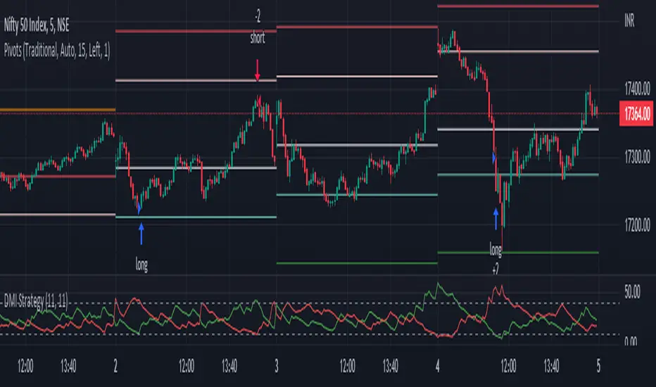
DMI StrategyThis strategy is based on DMI indicator. It helps me to identify base or top of the script. I mostly use this script to trade in Nifty bank options, even when the signal comes in nifty. It can be used to trade in other scripts as well. Pivot points can also be used to take entry. Long entry is taken when DI+(11) goes below 10 and DI-(11) goes above 40, whereas short entry is taken when DI-(11) goes below 10 and DI+(11) goes above 40.
For bank nifty, I take the trade in the strike price for which the current premium is nearby 300, with the SL of 20%. If premium goes below 10% I buy one more lot to average, but exit if the premium goes below 20% of the first entry. If the trade moves in the correct direction, we need to start trailing our stoploss or exit at the pre-defined target.
Please have a look at strategy tester to back test.
