Part 1 Support and Resistance 1. Introduction to Option Trading
Option trading is a type of derivatives trading where traders buy and sell options contracts rather than the underlying asset itself. An option is a financial contract that gives the holder the right, but not the obligation, to buy or sell an underlying asset at a specified price, called the strike price, on or before a specific date (expiration date). Options are widely used in equity, commodity, index, and currency markets.
Unlike traditional stock trading, option trading allows traders to leverage small amounts of capital to potentially earn higher returns. However, with this potential comes higher risk, especially in speculative strategies.
2. Key Terms in Option Trading
Before diving deeper, it’s essential to understand the terminology:
Call Option – Gives the buyer the right to buy the underlying asset at the strike price.
Put Option – Gives the buyer the right to sell the underlying asset at the strike price.
Strike Price (Exercise Price) – The price at which the underlying asset can be bought or sold.
Expiration Date – The date on which the option expires and becomes worthless if not exercised.
Premium – The price paid to buy the option.
Intrinsic Value – The difference between the underlying asset price and the strike price.
Time Value – The portion of the premium reflecting the remaining time until expiration.
In the Money (ITM) – A call option is ITM when the underlying price > strike price; a put option is ITM when the underlying price < strike price.
Out of the Money (OTM) – A call option is OTM when the underlying price < strike price; a put option is OTM when underlying price > strike price.
At the Money (ATM) – When the underlying price = strike price.
3. How Options Work
3.1 Call Options Example
Suppose a stock is trading at ₹100, and you buy a call option with a strike price of ₹105 for a premium of ₹2. If the stock rises to ₹115:
Intrinsic Value = 115 – 105 = ₹10
Profit = 10 – 2 (premium paid) = ₹8
If the stock stays below ₹105, the option expires worthless, and the loss is limited to the premium.
3.2 Put Options Example
Suppose the stock is at ₹100, and you buy a put option with a strike price of ₹95 for a premium of ₹3. If the stock falls to ₹85:
Intrinsic Value = 95 – 85 = ₹10
Profit = 10 – 3 (premium paid) = ₹7
If the stock stays above ₹95, the put expires worthless, and the loss is limited to the premium.
4. Types of Option Trading Participants
Buyers (Holders)
Pay a premium to gain the right to buy or sell.
Risk is limited to premium paid.
Sellers (Writers)
Receive a premium in exchange for obligation to buy or sell if exercised.
Risk can be unlimited in case of naked options, limited if covered.
5. Why Trade Options?
Option trading offers several advantages:
Leverage – Control a larger position with less capital.
Hedging – Protect against price movements in underlying assets.
Income Generation – Sell options to earn premiums (covered calls).
Flexibility – Apply strategies for bullish, bearish, or neutral markets.
Risk Management – Limit losses while maximizing profit potential.
HDBC trade ideas

Part 2 Support and Resistance1. Time Decay (Theta) in Action
Time decay erodes option premiums daily, faster near expiry. Example: An option priced ₹50 with 10 days left may lose ₹5 daily if underlying doesn’t move. This favors option sellers (who benefit from decay) and hurts option buyers (who need timely moves).
2. Volatility’s Influence on Options
Volatility is the heartbeat of option trading:
Implied Volatility (IV): Future expected volatility, priced into options.
Historical Volatility (HV): Past realized volatility.
If IV is high, premiums rise (good for sellers). Sudden IV drops after events (e.g., budget, results) can crush option buyers despite correct direction.
3. Advantages of Options Trading
Limited risk for buyers.
Lower capital requirement vs. buying stock.
Leverage enhances returns.
Hedging against market risk.
Multiple strategies for bullish, bearish, and neutral views.
This flexibility attracts both traders and investors.
4. Risks of Options Trading
Sellers face unlimited loss risk.
Buyers suffer time decay.
Sudden volatility crush (IV crash).
Complexity of Greeks.
Low liquidity in some stock options.
New traders often underestimate these risks.
5. Option Trading vs Futures Trading
Futures = Obligation to buy/sell at a fixed price.
Options = Right, not obligation.
Futures have linear P/L; options have asymmetric P/L.
Options require deeper risk management (Greeks, IV).
Both can be used together for hedging and speculation.
6. Single-Leg Option Strategies
Long Call: Bullish with limited risk.
Long Put: Bearish with limited risk.
Covered Call: Holding stock + selling call for income.
Protective Put: Holding stock + buying put for downside hedge.
These are basic building blocks.
7. Multi-Leg Option Strategies
Advanced traders combine options for defined outcomes:
Straddle: Buy call + put ATM → volatile move expected.
Strangle: Buy OTM call + OTM put → cheaper volatility bet.
Butterfly Spread: Limited risk, limited reward, range-bound outlook.
Iron Condor: Sell strangle + buy protection → income from low volatility.
8. Hedging with Options
Options allow investors to protect portfolios. Example: A mutual fund holding Nifty stocks can buy Nifty Puts to protect against a sudden crash. Farmers hedge crop prices with commodity options. Hedging reduces risk but costs premium.
9. Options in Intraday Trading
In India, options are heavily used for intraday speculation, especially in Nifty & Bank Nifty weekly contracts. Traders scalp premium moves, delta-neutral setups, or expiry-day theta decay. However, intraday option trading requires discipline due to extreme volatility.
10. Options in Swing and Positional Trading
Swing traders use options to play earnings results, events, or trends. Positional traders might use debit spreads (low risk) or credit spreads (income). Longer-dated options (LEAPS) are used for investment-style plays.

Introduction: Crafting the Trade Narrative1. The Essence of a Trade Narrative
At its core, a trade narrative is the story you tell yourself about the market and your position within it. Just as a novelist constructs a plot with characters, conflicts, and resolutions, a trader constructs a narrative that includes:
Market context: Understanding the broader economic, sectoral, and geopolitical factors influencing price movements.
Technical structure: The patterns, trends, and signals observed on charts.
Trading rationale: Why a particular position makes sense, including risk-reward assessments and potential catalysts.
Exit strategy: How the trade might conclude, whether through profit-taking, stop-loss execution, or reassessment.
Without this narrative, trades can become reactive and chaotic, influenced by emotions such as fear, greed, or impatience. A clearly crafted narrative, on the other hand, provides structure, discipline, and foresight. It turns speculation into informed decision-making.
2. Why Crafting a Narrative Matters
The importance of a trade narrative goes beyond technical analysis or market research. It serves several critical purposes:
2.1 Provides Clarity Amid Complexity
Financial markets are inherently complex and unpredictable. Prices fluctuate based on an enormous number of variables—macroeconomic data, corporate earnings, geopolitical tensions, central bank policies, and even social media sentiment. In such an environment, it is easy to feel overwhelmed. A trade narrative acts as a lens, filtering the noise and highlighting what truly matters for the specific trade.
2.2 Anchors Decisions in Logic, Not Emotion
One of the most common causes of trading failure is emotional decision-making. Fear and greed can lead to premature exits or holding losing trades for too long. A well-structured narrative anchors every decision in a logical framework, making it easier to adhere to your strategy even in turbulent markets.
2.3 Facilitates Learning and Growth
By documenting and reviewing your trade narratives, you create a record of your thinking and reasoning. Over time, this becomes an invaluable resource for learning—identifying patterns in your own behavior, refining strategies, and improving market intuition.
2.4 Enhances Communication
For professional traders or those managing funds, a clear trade narrative is essential for communicating ideas to colleagues, mentors, or clients. It allows others to understand your reasoning, evaluate your approach, and provide constructive feedback.
3. Core Components of a Trade Narrative
A compelling trade narrative combines multiple elements into a cohesive story. Let’s break down the essential components:
3.1 Market Context
Understanding the broader market is the first step. This includes:
Macro-economic trends: Interest rates, inflation data, GDP growth, employment statistics.
Sectoral trends: Which industries are performing well or poorly and why.
Geopolitical factors: Trade wars, sanctions, elections, and policy changes.
For instance, consider a trade in a technology stock. If the global economy is entering a phase of rising interest rates, tech stocks, which often rely on cheap capital for growth, may face downward pressure. Recognizing this context informs your trade narrative before you even look at charts.
3.2 Technical Analysis
Charts tell a story, and understanding that story is crucial. Technical analysis involves:
Trend analysis: Identifying bullish, bearish, or sideways market trends.
Support and resistance levels: Key price points where the market has historically reversed or paused.
Patterns and formations: Head and shoulders, triangles, flags, and candlestick patterns.
Volume analysis: Understanding the strength behind price movements.
Combining these elements provides a clear picture of where the market is and where it might go, forming the backbone of your narrative.
3.3 Trading Rationale
Once the market context and technical setup are understood, the trader must define the reasoning behind the trade. This includes:
Entry point: Why you are initiating the trade at this price.
Trade objective: Profit targets based on technical or fundamental factors.
Risk assessment: Stop-loss placement and maximum acceptable loss.
Catalysts: Events that could drive the price in your favor (earnings announcements, policy decisions, product launches).
This rationale transforms observations into actionable decisions.
3.4 Scenario Planning
Markets are unpredictable, so anticipating different outcomes is essential. A trade narrative should consider:
Best-case scenario: What you hope will happen and the potential profit.
Worst-case scenario: Risks and mitigation strategies.
Alternative scenarios: Market behaviors that might invalidate your assumptions and require a reassessment.
Scenario planning encourages flexibility, reducing the risk of tunnel vision.
3.5 Emotional and Psychological Considerations
Finally, a strong narrative acknowledges the trader’s emotions and mindset. This includes:
Awareness of personal biases (confirmation bias, recency bias, overconfidence).
Emotional triggers that might influence decision-making.
Discipline strategies to maintain adherence to the narrative under stress.
Psychology is often the invisible force that dictates outcomes more than charts or news.
4. Steps to Craft a Trade Narrative
Creating a trade narrative is not an abstract exercise; it is a practical, repeatable process. The following steps provide a structured approach:
Step 1: Research and Contextualize
Start with a broad understanding of the market and the instrument you plan to trade. This involves:
Reading macroeconomic reports and news.
Reviewing sector-specific developments.
Identifying key catalysts and events that could impact the trade.
Document your findings; clarity at this stage reduces guesswork later.
Step 2: Conduct Technical Analysis
Analyze price charts using tools such as:
Trend lines and channels.
Support and resistance zones.
Patterns and candlestick formations.
Moving averages and oscillators (RSI, MACD, etc.).
Summarize your technical observations as part of the narrative.
Step 3: Define the Trade Rationale
Explicitly state why the trade is being considered:
Entry price, stop-loss, and target levels.
Market signals or patterns supporting the trade.
Risk-reward ratio.
A clear rationale prevents impulsive adjustments mid-trade.
Step 4: Plan for Scenarios
Anticipate multiple outcomes:
Best, worst, and alternative scenarios.
Market conditions that could invalidate the trade.
Contingency plans for each scenario.
Scenario planning ensures readiness for uncertainty.
Step 5: Incorporate Psychological Preparedness
Recognize potential emotional pitfalls:
Stress triggers during market volatility.
Cognitive biases affecting judgment.
Pre-defined rules for sticking to or exiting the trade.
This psychological layer reinforces discipline and resilience.
Step 6: Document and Review
Finally, record the narrative in a journal. Include:
Market context and technical observations.
Rationale, targets, and risk assessment.
Scenario plans and emotional considerations.
Post-trade, review outcomes against the narrative to identify lessons learned and improve future decision-making.
5. Examples of Trade Narratives
Example 1: Short-Term Momentum Trade
Market context: Technology sector rally after strong earnings reports.
Technical analysis: Stock breaking above a key resistance at ₹1,500, with increasing volume.
Trade rationale: Enter at ₹1,510, target ₹1,560, stop-loss ₹1,490. Risk-reward ratio of 1:2.
Scenario planning:
Best case: Price hits ₹1,560 within 3 days.
Worst case: Price falls to ₹1,490; stop-loss triggered.
Alternative: Price consolidates between ₹1,500–₹1,520; reassess trend.
Psychology: Avoid chasing the trade if momentum fades; maintain discipline on stop-loss.
Example 2: Swing Trade on a Commodity
Market context: Crude oil prices expected to rise due to OPEC supply cuts.
Technical analysis: Strong support at $85, breakout from descending channel.
Trade rationale: Buy at $86, target $95, stop-loss $83.
Scenario planning: Monitor geopolitical developments; adjust stop-loss if global events change market dynamics.
Psychology: Be patient; swing trades require holding positions over multiple sessions without panic-selling.
6. The Benefits of Consistently Crafting Trade Narratives
Regularly creating trade narratives offers profound advantages:
Structured thinking: Encourages logical, disciplined, and systematic approaches.
Enhanced market intuition: Patterns become easier to recognize over time.
Reduced emotional trading: Anchors decisions in analysis, not impulses.
Better post-trade learning: Journaled narratives reveal strengths, weaknesses, and behavioral tendencies.
Professional credibility: Essential for managing others’ capital or communicating strategies effectively.
7. Common Mistakes in Trade Narratives
Despite their benefits, trade narratives can fail if misused. Common mistakes include:
Overcomplicating the story: Adding unnecessary details can obscure clarity.
Ignoring risk management: A narrative without defined stops is incomplete.
Neglecting emotional factors: Underestimating psychology can lead to unplanned deviations.
Failure to update: Markets evolve; narratives must be dynamic.
Confirmation bias: Only seeing evidence that supports the desired outcome, ignoring contrary signals.
Recognizing these pitfalls ensures the narrative remains practical, adaptable, and realistic.
8. Building a Narrative Culture
For professional trading teams or aspiring traders, fostering a narrative culture enhances performance. This involves:
Encouraging documentation and sharing of trade stories.
Reviewing narratives collectively to identify patterns and insights.
Integrating narrative-building into routine trading practice.
Rewarding disciplined adherence to structured plans rather than purely outcomes.
A culture of narratives cultivates disciplined thinking, teamwork, and continuous improvement.
Conclusion
Crafting the trade narrative is not merely a procedural step—it is the art and science of connecting analysis, intuition, and discipline into a coherent story that guides trading decisions. A strong narrative clarifies thought, anchors emotional responses, and transforms the chaos of the market into structured opportunity. By investing time in creating, reviewing, and refining trade narratives, traders cultivate a framework for sustained success, learning, and confidence.
The journey of mastering trade narratives is continuous. Each trade provides a lesson, each market condition offers new insights, and each review refines the story. Ultimately, the narrative is not just about the trade—it is about the trader, the mindset, and the disciplined approach that distinguishes success from failure in the dynamic world of financial markets.
Importance of Option Greeks in Trading and Risk Management1. Understanding Options and Their Intrinsic Complexity
Options are contracts that provide the holder with the right, but not the obligation, to buy or sell an underlying asset at a predetermined price (strike price) on or before a specific date (expiration). There are two primary types of options:
Call Options: Give the right to buy an asset.
Put Options: Give the right to sell an asset.
The value of an option is influenced by several factors, including:
Underlying asset price
Strike price
Time to expiration
Volatility of the underlying asset
Risk-free interest rate
Dividends (if any)
While these factors determine an option's price, the dynamic nature of the market requires traders to quantify how sensitive an option is to changes in these variables. This is where Option Greeks come into play. Greeks are named after Greek letters, each representing a specific sensitivity measure.
2. What Are Option Greeks?
Option Greeks are mathematical measures that indicate how the price of an option responds to various market factors. They provide traders with a way to quantify risk and manage exposure systematically.
The primary Option Greeks include:
Delta (Δ) – Sensitivity to underlying price changes
Gamma (Γ) – Sensitivity of Delta to underlying price changes
Theta (Θ) – Sensitivity to time decay
Vega (ν) – Sensitivity to volatility
Rho (ρ) – Sensitivity to interest rates
Each Greek serves a distinct purpose in options trading and risk management.
3. Delta (Δ): The Directional Sensitivity
Definition: Delta measures the rate of change of an option’s price relative to the change in the underlying asset's price. In simpler terms, it tells traders how much the option price is expected to move for a 1-unit move in the underlying asset.
Call options: Delta ranges from 0 to +1
Put options: Delta ranges from 0 to -1
Example:
If a call option has a Delta of 0.60 and the underlying stock moves up by $1, the option price is expected to rise by $0.60.
Importance in Trading:
Delta provides insight into the directional exposure of an options position. Traders can use Delta to:
Hedge stock positions
Estimate probability of an option expiring in the money
Construct Delta-neutral strategies
Delta Hedging:
Traders often aim to maintain a Delta-neutral portfolio to minimize the directional risk of underlying price movements. By adjusting the ratio of options and underlying assets, Delta hedging reduces the portfolio’s sensitivity to small price fluctuations.
4. Gamma (Γ): Measuring the Rate of Change of Delta
Definition: Gamma measures the rate of change of Delta with respect to changes in the underlying asset price. Essentially, Gamma tells traders how much Delta will change if the underlying price moves by one unit.
High Gamma: Delta is highly sensitive to price changes.
Low Gamma: Delta changes slowly.
Example:
If a call option has a Gamma of 0.05, a $1 increase in the stock price increases the Delta by 0.05.
Importance in Trading:
Gamma is crucial for understanding non-linear risk in options positions:
Helps traders gauge the stability of Delta.
High Gamma options are sensitive to price swings, requiring more active risk management.
Traders managing Delta-neutral portfolios monitor Gamma to adjust hedges frequently.
Practical Application:
Gamma is particularly significant for near-the-money options nearing expiration, as small price movements can cause rapid Delta changes.
5. Theta (Θ): Understanding Time Decay
Definition: Theta measures the sensitivity of an option’s price to the passage of time, also known as time decay. Theta is typically negative for long options positions because options lose value as expiration approaches, assuming all else remains constant.
Example:
If a call option has a Theta of -0.03, the option’s price will decrease by $0.03 per day due to time decay.
Importance in Trading:
Theta is critical for understanding the impact of time on option value:
Option sellers benefit from positive Theta as options lose value over time.
Option buyers experience negative Theta, requiring profitable moves in the underlying asset to offset time decay.
Practical Application:
Theta helps traders design income strategies such as:
Covered calls
Iron condors
Short straddles/strangles
Time decay can be a predictable source of profit if managed correctly.
6. Vega (ν): Sensitivity to Volatility
Definition: Vega measures the sensitivity of an option’s price to changes in implied volatility. Implied volatility reflects the market’s expectation of future price fluctuations in the underlying asset.
Example:
If a call option has a Vega of 0.10 and implied volatility rises by 1%, the option’s price increases by $0.10.
Importance in Trading:
Vega is critical for understanding the volatility risk:
High Vega options are more sensitive to changes in market volatility.
Traders use Vega to benefit from volatility trading, regardless of directional moves.
Practical Application:
Vega is central to strategies like:
Long straddles or strangles (profit from increased volatility)
Short volatility trades (profit from declining volatility)
Volatility management is especially important during earnings announcements, economic releases, or geopolitical events.
7. Rho (ρ): Interest Rate Sensitivity
Definition: Rho measures the sensitivity of an option’s price to changes in risk-free interest rates. Rho is more relevant for long-dated options, as interest rate fluctuations impact the present value of the strike price.
Example:
If a call option has a Rho of 0.05 and interest rates increase by 1%, the option price increases by $0.05.
Importance in Trading:
Rho is often less critical than Delta, Gamma, Theta, or Vega for short-term traders but is essential for long-term options strategies or interest-sensitive markets.
Practical Application:
Traders managing options in low-interest-rate vs. high-interest-rate environments monitor Rho to adjust risk exposures.
8. Interdependence of Greeks: The Dynamic Nature of Options
Option Greeks are not isolated; they interact dynamically:
Delta changes with Gamma.
Theta and Vega are interlinked as volatility affects time decay.
Multi-Greek analysis is necessary for sophisticated risk management.
For example, a near-the-money option with high Gamma and low Theta requires frequent adjustments to maintain Delta neutrality, whereas a far-out-of-the-money option with low Gamma and high Vega may be used for volatility plays.
9. Practical Applications in Trading
Option Greeks are critical tools for traders, hedgers, and portfolio managers. Some practical applications include:
9.1 Hedging Strategies
Delta Hedging: Neutralizes directional risk by balancing option and underlying asset positions.
Gamma Hedging: Ensures Delta remains stable as the underlying price moves.
Vega Hedging: Protects against volatility swings in options portfolios.
9.2 Risk Management
Identifying portfolio exposures across multiple Greeks.
Stress-testing scenarios: How would the portfolio behave under extreme price or volatility moves?
Adjusting positions dynamically to reduce undesirable risk.
9.3 Profit Optimization
Exploiting Theta decay through income-generating strategies.
Benefiting from volatility spikes using Vega-sensitive trades.
Structuring multi-leg trades with balanced Greeks for optimal risk-return.
10. Common Trading Strategies and Greeks Usage
Covered Call:
Positive Theta (time decay works in favor)
Delta is partially hedged
Protective Put:
Delta neutralizes stock exposure
Vega protects against volatility rise
Iron Condor:
Positive Theta (benefit from time decay)
Delta-neutral to minimize directional risk
Straddle/Strangle:
High Vega sensitivity (profit from volatility changes)
Requires Gamma and Theta monitoring
11. Advanced Risk Management Techniques Using Greeks
Multi-Greek Hedging:
Professional traders hedge multiple Greeks simultaneously to reduce exposure. Example: Balancing Delta, Gamma, and Vega to create a portfolio resilient to price, volatility, and time changes.
Dynamic Rebalancing:
Greeks change as market conditions evolve. Continuous monitoring and rebalancing of positions help maintain desired risk profiles.
Stress Testing and Scenario Analysis:
Using Greeks to simulate market scenarios and predict option portfolio performance. This is essential for protecting against tail risks and market shocks.
Portfolio Greeks Aggregation:
Large institutions aggregate Greeks across multiple options positions to quantify overall portfolio risk and identify vulnerabilities.
12. Importance for Retail and Institutional Traders
Option Greeks are indispensable tools for both retail traders and institutional investors:
Retail Traders:
Use Greeks to understand basic option sensitivities.
Implement strategies like covered calls, spreads, or protective puts with greater confidence.
Institutional Traders:
Conduct multi-dimensional risk management.
Hedge large portfolios using Delta, Gamma, Vega, Theta, and Rho.
Optimize portfolio performance using scenario analysis and stress testing.
13. Challenges in Using Option Greeks
While Greeks are highly useful, they come with challenges:
Complexity:
Requires understanding of multiple interacting factors.
New traders may find it overwhelming.
Dynamic Nature:
Greeks change with market movements, requiring constant monitoring.
Model Dependence:
Option Greeks are derived from pricing models (like Black-Scholes).
Model assumptions may not hold in extreme market conditions.
Liquidity and Slippage:
Large trades may not perfectly reflect calculated Greek hedges.
Despite these challenges, the benefits of using Option Greeks far outweigh the drawbacks for serious traders.
14. Conclusion
Option Greeks are fundamental tools for anyone serious about options trading and risk management. They quantify sensitivity to market variables such as price movements, volatility, time decay, and interest rates. By understanding and effectively managing Delta, Gamma, Theta, Vega, and Rho, traders can:
Reduce exposure to unwanted risks
Optimize returns
Implement complex hedging and trading strategies
Navigate volatile markets with confidence
In modern financial markets, where volatility and uncertainty are constants, Greeks offer a structured approach to understanding risk and opportunity in options trading. Mastering them is not merely a technical exercise—it is a crucial step toward becoming a disciplined, informed, and successful trader.
Option Greeks transform options from complex derivatives into measurable, manageable, and strategically valuable financial instruments, empowering traders to navigate the markets with precision and foresight.
Smart Money Secrets: Unlocking the Strategies of Market Insiders1. Understanding Smart Money
Smart money refers to capital controlled by institutional investors, hedge funds, central banks, high-net-worth individuals, or other financial entities that have access to superior information, resources, and analytical tools. Unlike retail traders, who often react emotionally to market events, smart money acts strategically, often positioning itself ahead of major market moves.
Key Characteristics of Smart Money
Informed Decision-Making: Smart money is guided by deep research, access to non-public or early public information, and advanced analytics.
Long-Term Strategy: While retail traders may chase short-term gains, smart money focuses on sustainable trends and risk-adjusted returns.
Market Influence: Large trades by institutional investors can move entire markets, influencing liquidity, price trends, and volatility.
Contrarian Behavior: Often, smart money goes against public sentiment, buying when retail panic sells and selling when retail greed drives prices up.
The essence of smart money is that it is strategically positioned, informed, and patient, making it a crucial concept for anyone seeking to understand market dynamics.
2. How Smart Money Moves
Smart money doesn’t just jump in randomly; its movements are deliberate, carefully calculated, and often hidden until the right moment.
a. Accumulation Phase
This is when smart money quietly starts buying a stock or asset without attracting attention. Retail traders may not notice, and prices may remain relatively flat. The goal is to accumulate a significant position at favorable prices.
Indicators of accumulation:
Increasing volume without major price movement.
Gradual upward trend after a prolonged downtrend.
Strong institutional buying reported in filings (e.g., 13F filings in the U.S.).
b. Markup Phase
Once enough positions are accumulated, smart money begins to push prices higher. This phase attracts retail traders and media attention. Prices may accelerate as momentum builds.
Indicators of markup:
Rising volume coinciding with price increase.
Breakouts above previous resistance levels.
Positive news and analyst upgrades (sometimes intentionally leaked).
c. Distribution Phase
Smart money slowly exits its positions, often selling to late-coming retail traders who are driven by hype. Despite the selling, the market may still appear bullish.
Indicators of distribution:
Volume spikes with minimal price change (selling into demand).
Repeated price rejection at key resistance levels.
Contradictory market sentiment (euphoria among retail investors).
d. Markdown Phase
Finally, the market corrects sharply as smart money has exited, leaving retail traders exposed. This phase often follows peaks in media coverage and public attention.
Indicators of markdown:
Price declines with increasing volume.
Negative news amplifying fear and panic selling.
Technical breakdowns through key support levels.
3. Tools to Track Smart Money
Identifying smart money movements requires using both technical and fundamental tools. Here are some widely used methods:
a. Volume Analysis
Volume spikes often indicate institutional activity. Unlike retail traders who trade in smaller sizes, large trades by institutions create noticeable volume patterns.
On-Balance Volume (OBV) and Volume Weighted Average Price (VWAP) can reveal buying or selling pressure not immediately visible in price charts.
b. Commitment of Traders (COT) Reports
COT reports, available for commodities and futures markets, show the positions of commercial and non-commercial traders. Sharp increases in commercial positions often signal smart money entering the market.
c. Options Market Activity
Unusual activity in call and put options may indicate that insiders or institutions are hedging large trades or anticipating significant moves.
Open interest changes and implied volatility spikes are useful signals.
d. Insider Trading Filings
In publicly traded companies, insider buying or selling can offer clues about smart money sentiment. While insiders may trade for personal reasons, consistent buying from executives can be a strong bullish signal.
e. Dark Pools
Large institutional trades are sometimes executed in private exchanges called dark pools to avoid affecting public prices. Tracking dark pool activity can give insights into hidden accumulation or distribution.
4. Psychology Behind Smart Money
Understanding smart money isn’t just about charts or filings—it’s also about human behavior and market psychology.
Fear and Greed: Retail traders often act on emotional impulses. Smart money exploits these emotions, buying when others fear and selling when others greed.
Patience and Discipline: Smart money waits for the right setup, unlike retail traders who chase immediate profits.
Contrarian Thinking: Going against the crowd is often a hallmark of smart money. Identifying overbought or oversold conditions allows them to capitalize on market sentiment extremes.
5. Strategies to Follow Smart Money
While replicating institutional strategies directly can be challenging due to scale and access, retail traders can learn and adapt techniques inspired by smart money principles.
a. Trend Following
Identify accumulation zones through volume and price analysis.
Ride trends in the markup phase while managing risk.
Avoid panic during minor corrections, focusing on broader smart money-driven trends.
b. Contrarian Investing
Look for areas where retail sentiment is extremely bullish (potential distribution) or extremely bearish (potential accumulation).
Use indicators like Fear & Greed Index, social media sentiment, and retail positioning metrics.
c. Risk Management
Smart money is always risk-aware. Proper position sizing, stop-loss strategies, and portfolio diversification help protect against unexpected moves.
Using tools like options for hedging can replicate professional risk management approaches.
d. Multi-Timeframe Analysis
Smart money operates across multiple timeframes—from intraday moves to multi-year positions.
Combining short-term and long-term charts can reveal where institutional positions are being built and unwound.
6. Common Smart Money Indicators
Several technical and market indicators are considered proxies for smart money activity:
Volume-Price Trend (VPT): Combines volume and price movement to indicate accumulation or distribution.
Accumulation/Distribution Line: Highlights whether a stock is being accumulated (bought) or distributed (sold).
Money Flow Index (MFI): A volume-weighted RSI that can reveal hidden buying/selling pressure.
VWAP (Volume Weighted Average Price): Tracks the average price weighted by volume—smart money often buys below VWAP and sells above it.
Conclusion
The secrets of smart money are not about mystical insider knowledge—they are about observation, discipline, and strategy. By studying market behavior, volume patterns, institutional filings, and psychological trends, retail traders can gain insights into the movements of the largest and most informed market players. While mimicking smart money directly is impossible for most individuals, understanding their methods, motives, and timing can provide a strategic edge, helping you make more informed and confident investment decisions.
Smart money strategies emphasize preparation, patience, and precision. By applying these principles consistently, retail traders can shift from reactive decision-making to proactive, informed, and strategic market engagement.
Risk-Free & Low-Risk Trading Strategies1. Understanding Risk in Trading
Before discussing strategies, it is essential to define what “risk” in trading entails. Risk refers to the probability of losing capital or the variance in returns. Common sources of trading risk include:
Market Risk: Price movements due to supply-demand dynamics or macroeconomic events.
Liquidity Risk: Difficulty in executing trades at desired prices.
Credit Risk: Counterparty default in derivative or forex transactions.
Operational Risk: Errors in execution, system failures, or regulatory breaches.
Event Risk: Sudden political, geopolitical, or natural events affecting markets.
Low-risk trading reduces exposure to these uncertainties, whereas risk-free trading strategies aim for almost certain outcomes, often through hedging or arbitrage.
2. Risk-Free Trading: Myth vs. Reality
While absolute risk-free trading is theoretically impossible in volatile markets, practically risk-free methods exist. These strategies rely on mechanisms like hedging, arbitrage, and government-backed instruments to eliminate or drastically reduce exposure.
2.1. Arbitrage Trading
Arbitrage is the simultaneous purchase and sale of an asset in different markets to exploit price discrepancies.
Types of arbitrage:
Stock Arbitrage: Buying a stock on one exchange where it is undervalued and selling on another where it is overvalued.
Forex Arbitrage: Exploiting currency price differences between two brokers or platforms.
Options Arbitrage: Using options strategies (like conversion or reversal trades) to lock in risk-free profits.
Example: If stock ABC trades at $100 on Exchange A and $101 on Exchange B, a trader can buy at $100 and sell at $101 simultaneously, capturing a risk-free $1 per share, minus transaction costs.
Pros: Almost zero market risk if executed correctly.
Cons: Requires high-speed execution, large capital, and minimal transaction costs.
2.2. Hedged Trading
Hedging involves taking offsetting positions to neutralize risk exposure.
Futures Hedging: A stockholder can sell futures contracts to protect against downside price movement.
Options Hedging: Buying put options against an equity holding to ensure a minimum exit price.
Forex Hedging: Holding positions in correlated currency pairs to minimize volatility risk.
Example: An investor holding 1000 shares of Company XYZ can buy put options with a strike price equal to the current market price. Even if XYZ falls sharply, the loss on shares is offset by gains on the options.
Pros: Reduces potential losses dramatically.
Cons: Hedging reduces potential profits; cost of options or futures must be considered.
2.3. Government Bonds and Treasury Instruments
Investments in government securities are often considered risk-free in terms of default (e.g., U.S. Treasury bonds).
Treasury Bills (T-Bills): Short-term government securities with fixed maturity.
Treasury Bonds: Long-term fixed-income instruments.
Inflation-Protected Securities (TIPS): Offer returns adjusted for inflation, protecting purchasing power.
Pros: Virtually no credit risk.
Cons: Returns are modest; inflation can erode gains if not using inflation-linked instruments.
3. Low-Risk Trading Strategies
While risk-free strategies focus on elimination of risk, low-risk strategies aim for capital preservation while achieving steady returns. These strategies balance risk and reward carefully.
3.1. Dollar-Cost Averaging (DCA)
Dollar-cost averaging involves investing a fixed amount at regular intervals, regardless of market conditions.
Smooths out volatility over time.
Reduces the emotional impact of market swings.
Works best in trending markets over the long term.
Example: Investing $500 monthly into an index fund. When the market is low, more units are purchased; when high, fewer units are bought, lowering average cost.
Pros: Simple, disciplined, and low-risk.
Cons: Not optimal for short-term trading; returns may be lower during strong bull markets.
3.2. Index Fund Investing
Instead of picking individual stocks, investing in broad market index funds spreads risk across multiple companies.
Reduces company-specific risk.
Tracks overall market growth.
Can be paired with DCA for better risk management.
Pros: Diversification, minimal research required, lower volatility.
Cons: Market risk still exists; less upside than high-growth stocks.
3.3. Blue-Chip Stock Trading
Blue-chip stocks are shares of large, financially stable companies with consistent performance.
Lower volatility than small-cap stocks.
Regular dividends can provide steady income.
Often resilient during economic downturns.
Pros: Low default risk, capital preservation.
Cons: Slower growth; requires proper selection and monitoring.
3.4. Covered Call Strategy
This options-based strategy involves holding a stock and selling call options on it.
Generates additional income through option premiums.
Slightly reduces downside exposure through received premiums.
Particularly effective in sideways or mildly bullish markets.
Example: Owning 100 shares of XYZ at $50 and selling a call option with a $55 strike. Premium collected provides cushion if stock drops.
Pros: Enhances income, lowers risk.
Cons: Caps upside gains; requires options knowledge.
3.5. Pair Trading
Pair trading is a market-neutral strategy where two correlated assets are traded simultaneously:
Long the undervalued asset.
Short the overvalued asset.
Example: If Stock A and Stock B historically move together but A rises while B falls, buy B and short A to profit when they revert.
Pros: Market risk minimized; suitable for volatile markets.
Cons: Requires statistical analysis and careful monitoring; capital-intensive.
4. Advanced Low-Risk Techniques
For more sophisticated traders, advanced methods further mitigate risk while preserving upside.
4.1. Volatility Trading
Low-risk traders can trade volatility rather than directional market moves:
Use VIX-linked ETFs or options to profit from volatility spikes.
Benefit from market stress without holding underlying assets.
Pros: Diversifies risk; potential profit in sideways or declining markets.
Cons: Complex; requires understanding implied and historical volatility.
4.2. Stop-Loss and Trailing Stop Orders
Setting stop-loss orders automatically exits a position if losses exceed a predetermined threshold.
Fixed Stop-Loss: Exits at a specific price.
Trailing Stop-Loss: Adjusts automatically as the market moves favorably.
Pros: Limits downside risk; enforces discipline.
Cons: Can trigger during short-term fluctuations; may miss recoveries.
4.3. Risk Parity Portfolio
This approach allocates capital across assets so that each contributes equally to overall portfolio risk.
Combines equities, bonds, commodities, and cash.
Adjusts exposure based on volatility.
Reduces portfolio-wide drawdowns.
Pros: Balanced risk; improves long-term stability.
Cons: Complex; requires continuous rebalancing.
5. Risk Assessment and Management Tools
No strategy is complete without proper risk assessment and management techniques:
Value-at-Risk (VaR): Estimates potential loss over a period with a confidence interval.
Beta Coefficient: Measures a stock’s volatility relative to the market.
Sharpe Ratio: Assesses risk-adjusted return.
Stress Testing: Simulates extreme market scenarios to evaluate strategy resilience.
Practical Tip: Combine quantitative tools with qualitative judgment. For example, even a historically low-beta stock may experience sudden drops during geopolitical crises.
6. Practical Examples of Risk-Free & Low-Risk Portfolios
Example 1: Risk-Free Arbitrage
Buy stock at $100 in Exchange A.
Sell at $101 in Exchange B.
Trade size: 1,000 shares.
Profit: $1,000 minus transaction costs.
Outcome: Nearly risk-free profit.
Example 2: Low-Risk Dividend Strategy
Portfolio: 60% blue-chip dividend stocks, 30% bonds, 10% cash.
Dividend yield: 3–5%.
Potential capital appreciation: Moderate.
Risk: Low, as losses are cushioned by bonds and cash.
Example 3: Hedged Options Strategy
Own 1,000 shares of XYZ at $50.
Buy 10 put options with strike $50.
Market drops to $40; put options gain, offsetting stock loss.
Outcome: Capital preservation, limited downside.
7. Key Principles for Low-Risk & Risk-Free Trading
Diversification: Spread capital across assets and sectors to reduce concentration risk.
Hedging: Use derivatives or correlated instruments to offset potential losses.
Discipline: Stick to strategies; avoid emotional trades.
Monitoring: Track markets, news, and portfolio performance regularly.
Leverage Caution: Avoid excessive leverage; amplifies both gains and losses.
Liquidity Awareness: Ensure positions can be exited quickly if needed.
Continuous Learning: Markets evolve; strategies must adapt.
8. Limitations and Realistic Expectations
Risk-free profits are usually small and capital-intensive.
Low-risk strategies sacrifice some upside potential for safety.
Market anomalies, slippage, or transaction costs can erode expected gains.
Even highly diversified portfolios are not immune to systemic crises.
Mindset Tip: Focus on capital preservation first, then on incremental gains. Compounding small, consistent returns often outperforms high-risk speculation over time.
9. Conclusion
Risk-free and low-risk trading strategies are vital for traders seeking consistent returns with capital protection. While no method guarantees absolute safety, techniques like arbitrage, hedging, DCA, diversification, and options-based strategies can significantly reduce exposure.
Successful low-risk trading is less about chasing big profits and more about disciplined execution, risk assessment, and strategy adaptation. By combining these methods with proper monitoring and financial tools, traders can navigate market volatility confidently, protecting capital while capturing incremental gains.
Final Thought: In trading, preserving what you earn is as important as earning itself. Low-risk and risk-free strategies are not just methods—they’re a mindset that prioritizes security, consistency, and long-term growth.
HDFCBANK 1D Time frame📍 Current Price & Range
Current price: ₹964.20
Day’s High / Low: ₹968.20 / ₹955.50
52-week High / Low: ₹1,018.85 / ₹806.50
🔍 Key Levels (with current context)
Immediate support: ₹955-₹958
Stronger support: ₹945-₹950
Immediate resistance: ₹970-₹975
Next resistance: ₹980-₹985
Major psychological resistance: ₹1,000+
📊 Indicators & Momentum
Price is near resistance zone (₹964-₹967), showing hesitation.
Holding above ₹955 is important for stability.
Price is below the 50-day moving average → short-term weakness.
Still above the 200-day moving average → long-term structure remains intact.
RSI around 40-45 → momentum is neutral to slightly weak.
🔮 Possible Scenarios
Bullish breakout: Above ₹975-₹980 with volume → upside toward ₹1,000–₹1,018.
Sideways: Between ₹955–₹975 until a decisive breakout.
Bearish pullback: Below ₹955 → could slide toward ₹945-₹950 or even ₹940.
👉 Outlook: At the current level (₹964), the stock is sitting close to resistance. It needs strength above ₹975 to turn bullish; otherwise, it risks drifting back toward ₹955 support.

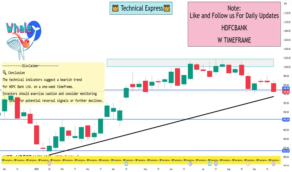
HDFCBANK 1 Week View📉 Technical Indicators
Relative Strength Index (RSI): Approximately 35.08, indicating the stock is nearing oversold conditions but not yet in the oversold zone.
Moving Average Convergence Divergence (MACD): Around -6.02, suggesting a bearish trend.
Moving Averages:
5-day EMA: ₹957.70 (Sell)
10-day EMA: ₹963.20 (Sell)
20-day EMA: ₹961.06 (Sell)
50-day EMA: ₹981.06 (Sell)
100-day EMA: ₹974.24 (Sell)
200-day EMA: ₹921.92 (Buy)
The short-term moving averages are indicating sell signals, while the long-term 200-day EMA is showing a buy signal.
Pivot Points:
Support Levels: ₹929.82 (S3), ₹936.53 (S2), ₹943.52 (S1)
Resistance Levels: ₹957.22 (R1), ₹963.93 (R2), ₹970.92 (R3)
These levels can help identify potential price reversal points.
📊 Price Action
The stock closed at ₹945.05 on September 26, 2025, marking a 0.51% decline from the previous close. Over the past week, the share price has decreased by 2.26%.
⚠️ Recent Developments
HDFC Bank is currently facing regulatory challenges, including a ban by the Dubai Financial Services Authority from accepting new clients or initiating new business activities through its branch at the Dubai International Financial Centre. This could impact investor sentiment and the bank's international operations.
🔍 Conclusion
The technical indicators suggest a bearish trend for HDFC Bank Ltd. on a one-week timeframe. Investors should exercise caution and consider monitoring the stock for potential reversal signals or further declines.
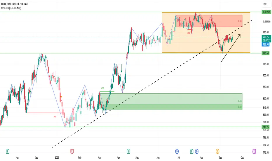
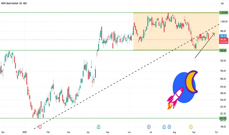
Smart Money Play: Watching HDFC Bank’s Bullish ZoneTrading Idea: HDFC Bank (NSE: HDFCBANK)
Price is currently trading around ₹976 after a recent pullback.
Key Observations:
Break of Structure (BOS) confirms bullish market structure.
Liquidity sweep around recent highs.
Daily Fair Value Gap (FVG) spotted between ₹910–₹930.
Bullish Order Block at ₹800–₹830 acting as strong higher timeframe support.
Plan:
Expecting a retracement into the Daily FVG zone (₹910–₹930).
If price reacts bullishly here, potential upside rally towards ₹1,040+.
Confirmation: Look for bullish reversal candles or demand zone rejections inside FVG.
Risk Management:
Aggressive entry: near FVG zone (₹910–₹930).
Conservative entry: only after bullish confirmation.
Stop-loss: below ₹890.
Targets: First TP at ₹990, extended TP at ₹1,040.
Bias: Bullish (after retracement).
Disclaimer: This is not financial advice. For educational purposes only. Please do your own research or consult with a financial advisor before making any investment decisions.

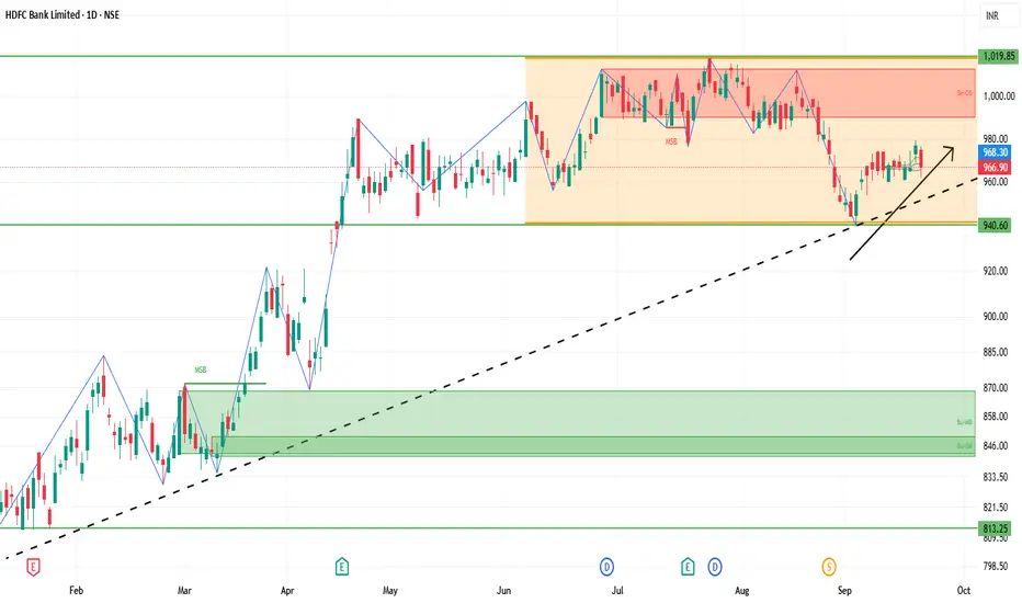
HDFCBANK 1D Time frameCurrent Stock Price
Current Price: ₹966.85
Day’s Range: ₹965.15 – ₹974.40
52-Week Range: ₹806.50 – ₹1,018.85
Market Cap: ₹14.88 lakh crore
P/E Ratio: 21.03
EPS (TTM): ₹45.97
Dividend Yield: 1.13%
Book Value: ₹339.84
📈 Trend & Outlook
Short-Term Trend: Mildly bullish; stock showing positive movement in recent sessions.
Resistance Levels: ₹974.40 (day’s high), ₹1,018.85 (52-week high).
Support Levels: ₹965.15 (day’s low), ₹950.00 (recent low).
Investor Sentiment: Positive, supported by institutional buying and favorable outlook.
🧭 Key Notes
Stock has room to move higher if it breaks near-term resistance.
If it falls below support, downside may extend to ₹950 or lower.
Overall, bulls are slightly stronger, but watch resistance for profit booking.
HDFCBANK 1D Time framePrice Action
Current Price: ₹967.10 (approx)
Day’s Range: ₹965 – ₹970
52-Week Range: ₹806.50 – ₹1,018.85
🔹 Support & Resistance
Immediate Support: ₹960 – ₹958
Next Support: ₹954 – ₹950
Immediate Resistance: ₹970 – ₹975
Higher Resistance: ₹980

Part 1 Ride The Big Moves Part 1: Introduction to Option Trading
Option trading is a cornerstone of modern financial markets, offering traders and investors the flexibility to manage risk, speculate on price movements, and generate income. At its core, an option is a financial derivative—a contract that derives its value from an underlying asset, which can include stocks, indices, commodities, currencies, or ETFs. Unlike owning the underlying asset directly, an option provides the right—but not the obligation—to buy or sell that asset at a predetermined price within a specific time frame.
There are two primary types of options:
Call Options: Grant the buyer the right to purchase the underlying asset at a specific price, known as the strike price, before or on the option’s expiration date.
Put Options: Grant the buyer the right to sell the underlying asset at the strike price within a specified period.
The price paid to acquire an option is called the premium. This premium reflects the market’s perception of the likelihood that the option will end up profitable (in the money). Premiums are influenced by various factors, including the asset’s current price, strike price, time to expiration, volatility, interest rates, and dividends.
Option trading serves several purposes:
Hedging: Investors use options to protect existing positions against adverse price movements. For instance, owning put options can act as insurance against a decline in stock prices.
Speculation: Traders seeking profit from short-term price movements can leverage options to gain higher exposure with limited capital compared to buying the underlying asset outright.
Income Generation: Writing (selling) options allows investors to collect premiums, thereby generating income. Covered call strategies, for example, are widely used to earn consistent returns on long stock holdings.
Options differ from futures contracts in key ways. Futures obligate the buyer to purchase (or the seller to sell) the underlying asset at a future date, regardless of market conditions. Options, conversely, provide a choice without mandatory execution, giving traders more strategic flexibility. This asymmetry between risk and reward makes option trading unique and complex, requiring a strong grasp of market behavior, probability, and timing.
The evolution of option markets has been significant. Initially, options were traded over-the-counter (OTC), with bespoke contracts negotiated privately. With the establishment of standardized exchanges like the Chicago Board Options Exchange (CBOE) in 1973, options trading became more accessible, liquid, and regulated, paving the way for retail participation and complex strategies.
Part 2: Key Concepts and Terminologies
Understanding option trading requires familiarity with several fundamental concepts and terms:
Strike Price: The fixed price at which the underlying asset can be bought (call) or sold (put). It is central to determining whether an option is profitable at expiration.
Expiration Date: The date on which the option contract ceases to exist. Options are classified based on their lifespan:
Short-term options: Expire in days to weeks.
Long-term options: Also known as LEAPS, they can extend up to three years.
In the Money (ITM), At the Money (ATM), Out of the Money (OTM):
ITM: Option has intrinsic value (e.g., a call option’s strike price is below the current stock price).
ATM: Strike price equals the underlying asset’s current price.
OTM: Option lacks intrinsic value but may have time value.
Intrinsic and Extrinsic Value: Intrinsic value reflects the real, immediate value of an option (profit if exercised today). Extrinsic value is the premium over intrinsic value, factoring in time, volatility, and market conditions.
Volatility: A measure of price fluctuations of the underlying asset. Higher volatility increases option premiums due to greater potential for profit.
Option Greeks: These are critical tools to quantify risks and potential rewards:
Delta: Sensitivity of option price to changes in the underlying asset price.
Gamma: Rate of change of delta.
Theta: Time decay, or how an option’s value decreases as expiration nears.
Vega: Sensitivity to volatility changes.
Rho: Sensitivity to interest rate changes.
Additionally, American vs. European options is an important distinction. American options can be exercised anytime until expiration, whereas European options can only be exercised at expiration. While this sounds straightforward, it profoundly affects pricing and strategy.
Option contracts are standardized in terms of quantity, strike prices, and expiration cycles on exchanges. This standardization allows traders to combine options in sophisticated strategies such as spreads, straddles, and butterflies.

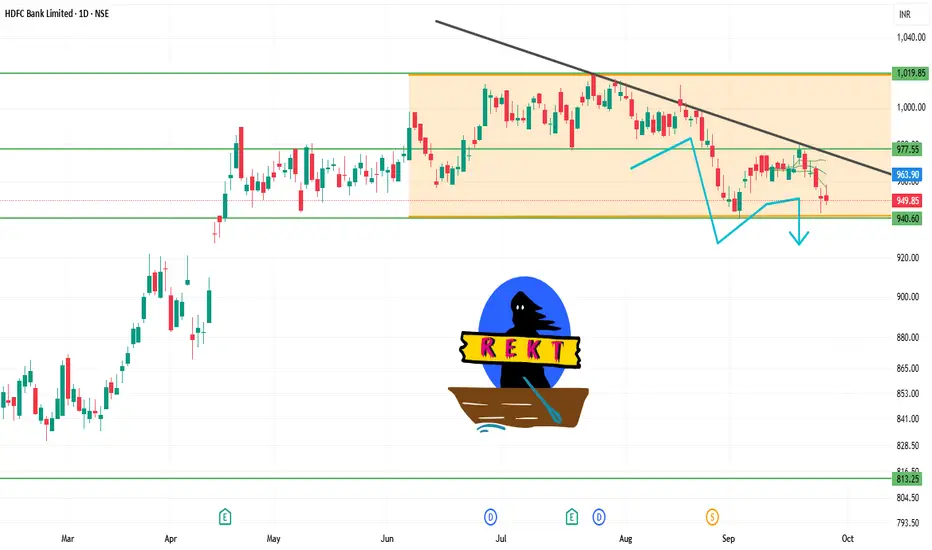
HDFCBANK 1D Time frame📊 Daily Snapshot
Closing Price: ₹949.20
Day’s Range: ₹947.40 – ₹958.00
Previous Close: ₹957.20
Change: Down –0.52%
52-Week Range: ₹806.50 – ₹1,018.85
Market Cap: ₹14.6 lakh crore
P/E Ratio: 20.66
Dividend Yield: 2.32%
EPS (TTM): ₹45.97
Beta: 0.92 (indicating lower volatility)
🔑 Key Technical Levels
Support Zone: ₹947.40 – ₹950.00
Resistance Zone: ₹957.20 – ₹960.00
All-Time High: ₹1,018.85
📈 Strategy (1D Timeframe)
1. Bullish Scenario
Entry: Above ₹957.20
Stop-Loss: ₹947.40
Target: ₹965.00 → ₹970.00
2. Bearish Scenario
Entry: Below ₹947.40
Stop-Loss: ₹957.20
Target: ₹940.00 → ₹935.00
HDFC Bank AnalysisHDFC is trading in a sideways range. It will give big move on breakout of 1018 on Upside and 904 on Down side. BB is Sideways.

HDFC BANK LONG TERM PICTURE AS PER MY VIEWon daily tf price changed character and turned -ve
There are some support areas on weekly tf from where we can expect a reversal

HDFCBANK 1D Time frame📊 Current Snapshot
Current Price: Around ₹967
Day Range: ₹962 – ₹976
52‑Week Range: High ~ ₹1,018, Low ~ ₹805
Volume: Slightly above recent average, showing decent trading interest
🔍 Support & Resistance
Immediate Resistance: ₹975 – ₹983
Higher Resistance: ₹989 – ₹990
Immediate Support: ₹960 – ₹954
Lower Support: ₹946
⚙️ Indicators & Trend
RSI / Stochastic: Neutral to slightly bearish, indicating mild selling pressure
Pivot Level: Around ₹968 – ₹969, meaning price is near equilibrium
Moving Averages: Mixed signals; short-term MAs under slight pressure, long-term trend still intact
🎯 Possible Scenarios
Bullish Case: Break and sustain above ₹980 → next target ₹990+
Bearish Case: Fail at resistance → pullback toward ₹960‑₹954; below ₹954 → possible drop to ₹946
⚠️ Key Points
Resistance zones are tight and need strong volume for a breakout
Price near pivot levels may lead to short-term sideways movement or volatility
Confirmation from trading volume is important for trend sustainability
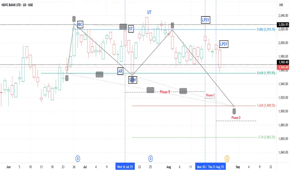
HDFC study with WYCOFF incorporating harmonic patternHDFC 1964 - A study with WYCOFF incorporating harmonic pattern suggests price target1 at 1908and target 2 at 1862 with resistance 1994.
HDFCBANK 1D Time frameTrend
Trading around ₹967 – ₹970.
Stock is in a consolidation phase for the past few months.
Long-term trend is intact since it is above the 200-day moving average.
Support Levels
₹960 – ₹965 → immediate support zone.
₹945 – ₹950 → stronger support; if this breaks, stock may weaken further.
Resistance Levels
₹970 – ₹975 → immediate resistance; stock is struggling to cross this area.
₹980 – ₹992 → next major resistance; breakout above this could open path to ₹1,020.
Indicators
RSI near 55 → neutral to mildly bullish, not overbought.
MACD positive, showing some upward momentum.
Short-term moving averages are mixed, but long-term support remains strong.
Price Action
Range-bound between ₹960 – ₹975.
Breakout or breakdown from this range will decide the next trend.
✅ Facts & Insights
Fact 1: Above ₹975, HDFC Bank can rally towards ₹980 – ₹992 and possibly ₹1,020.
Fact 2: Below ₹960, stock may slip to ₹945 – ₹950, and deeper to ₹920 – ₹900 if weakness continues.
Fact 3: Long-term outlook remains positive, but short-term is sideways until a breakout.
Rate Hikes: Interest Rates vs. Inflation1. Introduction: The Relationship Between Interest Rates and Inflation
At its core, inflation refers to the sustained rise in the general price level of goods and services in an economy over time. When prices rise faster than incomes, purchasing power declines, impacting consumers, businesses, and investors.
Interest rates, on the other hand, represent the cost of borrowing money or the reward for saving. Central banks, like the Federal Reserve (US), Reserve Bank of India (RBI), or European Central Bank (ECB), manipulate policy interest rates to influence economic activity.
Key relationship:
When inflation rises beyond the central bank’s target, interest rates are often increased (a process called a “rate hike”) to curb spending and borrowing.
Conversely, during periods of low inflation or deflation, central banks may lower interest rates to stimulate demand.
2. How Central Banks Use Rate Hikes to Control Inflation
2.1 The Mechanism of Monetary Policy
Central banks influence inflation primarily through monetary policy tools. Rate hikes are part of tightening monetary policy, which affects the economy in several ways:
Borrowing Costs Increase: Higher interest rates make loans for businesses and consumers more expensive. This reduces spending on big-ticket items like houses, cars, and capital investments.
Savings Become Attractive: As banks offer higher returns on deposits, consumers may save more and spend less, reducing aggregate demand.
Currency Appreciation: Higher rates often attract foreign capital, strengthening the domestic currency. A stronger currency makes imports cheaper, which can reduce imported inflation.
Expectations Management: Rate hikes signal the central bank’s commitment to controlling inflation, which can influence wage negotiations, business pricing decisions, and consumer behavior.
2.2 Transmission Mechanism
The impact of rate hikes on inflation is not instantaneous. It passes through the economy via the interest rate transmission mechanism, which works through:
Credit channel: Expensive credit discourages borrowing.
Asset price channel: Rising rates reduce stock and real estate valuations, leading to lower wealth effect and reduced spending.
Exchange rate channel: Higher rates attract capital inflows, boosting the currency, reducing import costs, and easing inflation.
Typically, the full impact of a rate hike is observed over 12–24 months.
3. Types of Inflation and Rate Hikes
Not all inflation is the same, and the effectiveness of interest rate hikes depends on the source of inflation:
3.1 Demand-Pull Inflation
Occurs when aggregate demand exceeds supply.
Example: Booming economy with high consumer spending.
Rate hike effect: Very effective, as higher borrowing costs reduce spending.
3.2 Cost-Push Inflation
Occurs when production costs rise, e.g., due to higher wages, oil prices, or supply chain disruptions.
Rate hike effect: Less effective, as inflation is supply-driven rather than demand-driven.
3.3 Built-in Inflation
Caused by adaptive expectations, where past inflation influences future wage and price increases.
Rate hike effect: Moderate, but signaling by the central bank can anchor inflation expectations.
4. Historical Perspective on Rate Hikes and Inflation
Studying historical trends helps illustrate how interest rate adjustments influence inflation:
4.1 US Experience
1970s: Stagflation with double-digit inflation. The Fed raised rates sharply under Paul Volcker, with the federal funds rate peaking at ~20%. Inflation eventually came under control, but the economy experienced a severe recession.
2000s–2020s: Post-2008 financial crisis, rates were near zero to stimulate the economy. Inflation remained low, demonstrating that low rates don’t always trigger high inflation if other conditions (like excess capacity) persist.
4.2 Indian Experience
RBI uses repo rates to manage inflation, targeting CPI (Consumer Price Index) inflation around 4% ±2%.
Example: During 2010–2013, high food and fuel inflation prompted the RBI to raise repo rates to curb prices, stabilizing inflation over time.
4.3 Emerging Markets
Rate hikes in emerging markets often have the dual objective of controlling inflation and maintaining currency stability.
Over-tightening can trigger slowdowns, especially in economies with high debt levels.
5. Rate Hikes vs. Economic Growth
While rate hikes are effective in controlling inflation, they have trade-offs:
5.1 Impact on Investment
Higher borrowing costs reduce business investments in new projects.
Stock markets often react negatively, especially for high-debt sectors.
5.2 Impact on Consumers
Loans (housing, education, personal loans) become more expensive, reducing disposable income.
Luxury and discretionary spending decline.
5.3 Risk of Recession
Aggressive rate hikes can slow the economy too much, leading to contraction.
Policymakers must balance inflation control with growth sustainability.
6. Rate Hikes and Financial Markets
Financial markets react dynamically to rate hikes:
6.1 Stock Markets
Typically, rate hikes are bearish for equities as corporate profits may decline due to higher financing costs.
Growth stocks (tech) are more sensitive than value stocks.
6.2 Bond Markets
Bond prices fall as yields rise.
Investors shift to shorter-duration bonds during rate hike cycles.
6.3 Forex Markets
Domestic currency tends to strengthen as higher rates attract foreign capital.
This can impact export competitiveness but reduce import-driven inflation.
6.4 Commodities
Commodities priced in USD may decline as stronger currency reduces local demand.
Gold often falls during rate hikes because it doesn’t yield interest.
7. Rate Hikes in a Global Context
Interest rate policy in one country can influence others:
7.1 Spillover Effects
Higher US rates often lead to capital outflows from emerging markets.
Countries may raise rates in tandem to protect their currency and control inflation.
7.2 Global Inflation Trends
Oil prices, supply chain disruptions, and geopolitical events can override local rate hikes.
Central banks must consider global factors while adjusting rates.
8. Challenges in Managing Inflation Through Rate Hikes
8.1 Lag Effect
Monetary policy effects are delayed; policymakers often act based on inflation expectations rather than current data.
8.2 Supply-Side Constraints
Rate hikes cannot solve inflation caused by supply shortages or geopolitical disruptions.
8.3 Debt Burden
Economies with high corporate or household debt may be more sensitive to rate hikes, risking defaults.
8.4 Policy Communication
Miscommunication can destabilize markets. Clear forward guidance is crucial.
Conclusion
Interest rates and inflation are intricately linked. Rate hikes are a powerful tool to control inflation, but they come with trade-offs for growth, investment, and financial markets.
Key takeaways:
Rate hikes reduce demand and curb inflation but may slow growth.
Demand-pull inflation responds better to rate hikes than supply-driven inflation.
Timing, magnitude, and communication of rate hikes are crucial.
Global interdependencies mean domestic rate policy must consider international factors.
Investors and traders must adapt strategies in response to rate hikes, balancing risk and opportunity.
Ultimately, the goal of rate hikes is stability—stable prices, sustainable growth, and predictable financial markets. Policymakers walk a delicate tightrope, balancing inflation control with the need to foster economic activity, making the study of interest rates versus inflation an essential part of modern finance and economics.
Part 2 Candle Stick Pattern Types of Options
There are two primary types of options:
a) Call Options
Gives the holder the right to buy an underlying asset at a specified strike price.
Investors buy calls when they expect the underlying asset price to rise.
Example: If stock ABC is trading at ₹100 and you buy a call with a strike price of ₹110, you profit if ABC rises above ₹110 plus the premium paid.
b) Put Options
Gives the holder the right to sell an underlying asset at a specified strike price.
Investors buy puts when they expect the underlying asset price to fall.
Example: If stock XYZ is trading at ₹200 and you buy a put with a strike price of ₹190, you profit if XYZ falls below ₹190 minus the premium paid.
Option Pricing and Valuation
Option pricing is crucial in determining potential profits and risks. Two main components influence the price of an option:
a) Intrinsic Value
For a call option: Current Price – Strike Price
For a put option: Strike Price – Current Price
Intrinsic value is zero if the option is out-of-the-money.
b) Time Value
Time value depends on:
Time to Expiry: Longer time increases the premium.
Volatility: Higher volatility increases the likelihood of profitable movements.
Interest Rates: Small effect on option premiums.
Dividends: Impact options on dividend-paying stocks.
c) Black-Scholes Model
Widely used for European-style options pricing.
Formula incorporates current stock price, strike price, time to expiration, volatility, and risk-free rate.
d) Greeks
Measures the sensitivity of option prices to various factors:
Delta: Sensitivity to the underlying asset price.
Gamma: Rate of change of delta.
Theta: Time decay effect.
Vega: Sensitivity to volatility.
Rho: Sensitivity to interest rate changes.

Market Structure Secrets: Trade Like Institutional Players1. Understanding Market Structure
1.1 What is Market Structure?
Market structure refers to the arrangement of price movements over time. It provides insight into supply and demand dynamics, trend direction, and potential reversals. Every market—stocks, forex, crypto, or commodities—follows the same fundamental laws of supply and demand.
Market structure analysis is about identifying three key components:
Trends: The market rarely moves sideways forever. Prices either trend upwards (bullish) or downwards (bearish).
Support and Resistance Levels: Price zones where buying or selling interest is concentrated.
Market Phases: Accumulation, markup, distribution, and markdown.
1.2 Why Institutions Focus on Market Structure
Institutions trade based on order flow and liquidity pools. They do not guess market direction; they react to the behavior of other participants. By understanding market structure:
They know where liquidity exists (areas where stop losses are clustered).
They identify swing highs and lows, which are often targets for large orders.
They detect market imbalances that can be exploited.
Retail traders often lose because they ignore these structural cues, buying near highs or selling near lows, instead of waiting for the market to reveal its true intention.
2. The Building Blocks of Market Structure
2.1 Trends and Swings
Markets move in waves, forming swing highs and swing lows:
Higher Highs and Higher Lows: Bullish trend
Lower Highs and Lower Lows: Bearish trend
Sideways Movement: Consolidation
Institutions track these swings meticulously. They accumulate during consolidation and exploit breakouts once the market direction is clear.
2.2 Support and Resistance
Support: A price zone where demand outweighs supply.
Resistance: A price zone where supply outweighs demand.
Institutions often place large orders around these zones. Retail traders frequently misinterpret these levels, leading to false breakouts, which are prime hunting grounds for institutional traders.
2.3 Liquidity Zones
Liquidity is the fuel of the market. Institutional players look for areas with clustered stop-loss orders because triggering these orders allows them to enter or exit positions efficiently.
Common liquidity zones:
Recent swing highs/lows
Round numbers (e.g., 100, 150 in stocks)
Support/resistance levels
Understanding liquidity zones helps anticipate market moves that seem “unexpected” to retail traders.
3. The Institutional Footprint
Institutions leave footprints in the market. While retail traders rely on indicators, institutional players focus on price action and volume to gauge activity.
3.1 Order Blocks
An order block is a price area where institutions accumulate or distribute positions. It often precedes a strong market move.
Bullish Order Block: Precedes an upward rally
Bearish Order Block: Precedes a downward drop
Recognizing these zones allows traders to enter trades in harmony with institutional flows, improving their odds of success.
3.2 Market Phases Explained
Markets move through predictable phases:
Accumulation Phase: Institutions quietly buy without pushing prices significantly.
Markup Phase: After enough accumulation, prices rise rapidly.
Distribution Phase: Institutions gradually sell to retail traders at higher prices.
Markdown Phase: Prices fall as retail traders panic sell.
Identifying the phase helps you trade with the smart money instead of against it.
4. Trading Like Institutional Players
4.1 Concept of “Smart Money”
Smart money refers to capital controlled by large players who influence price action. Trading like smart money means:
Waiting for the institutional setup (order blocks, liquidity grabs)
Avoiding emotional decisions
Using market structure to find high-probability trades
4.2 Key Institutional Trading Strategies
4.2.1 Breakout and Retest
Institutions often push price beyond support or resistance to trigger stops, then let it retrace. Retail traders chase the breakout, while institutions enter at the retest for optimal risk-reward.
Steps:
Identify a breakout from a key level.
Wait for price to retest the level.
Enter trade in the direction of the breakout.
4.2.2 Supply and Demand Zones
Institutions buy from areas of high supply and sell at areas of high demand. These zones often coincide with:
Previous consolidation areas
Swing highs/lows
Key Fibonacci retracement levels
Trading these zones aligns you with institutional intentions.
4.2.3 Liquidity Hunts
Institutions deliberately push price into stop-loss clusters to capture liquidity. Recognizing these hunts allows you to:
Avoid being trapped
Trade the reversal after stops are triggered
Example: Price pushes below a swing low, triggers stops, then reverses sharply upward.
4.2.4 Trend Following
Institutions trend-follow but only when risk is optimal. They enter after:
Consolidation
Liquidity capture
Confirmation of institutional order flow
Trend-following blindly is risky; trend-following smartly requires market structure knowledge.
4.3 Practical Trade Setups
4.3.1 Order Block Entry
Identify bullish/bearish order blocks
Wait for price to return to the block
Confirm with price rejection patterns (pin bars, engulfing candles)
Enter trade with tight stop loss and realistic target
4.3.2 Breakout-Retest Entry
Spot breakout above resistance or below support
Wait for retest of the level
Look for volume confirmation
Enter in the direction of breakout
4.3.3 Liquidity Grab Reversal
Identify probable stop-loss clusters
Watch for price to violate these levels
Confirm reversal using price action
Enter trade with proper risk management
5. Risk Management Like an Institution
Institutions protect their capital meticulously. They rarely risk more than a small fraction of their capital on a single trade. Key takeaways:
Use stop-loss orders wisely: Place them outside market noise, not arbitrary points.
Calculate risk-reward: Aim for setups where potential reward is at least 2–3 times the risk.
Position sizing: Adjust trade size based on confidence and market volatility.
Avoid overtrading: Institutions wait for high-probability trades, not constant action.
Conclusion
Trading like an institutional player is not about complexity; it’s about understanding market behavior, respecting structure, and managing risk. The retail trader often loses because they react emotionally, chase price, or rely too heavily on lagging indicators. In contrast, institutions:
Follow the market’s natural rhythm
Target liquidity zones
Trade with disciplined risk management
Act based on structure, not guesswork
By studying market structure, learning institutional footprints, and practicing disciplined execution, retail traders can gain an edge. Mastery comes from observation, patience, and continuous refinement.
Trading like an institution doesn’t guarantee instant profits, but it aligns you with the smart money, giving you the highest probability of success.

HDFCBANK 1D Time frame📉 Current Market Snapshot
Closing Price: ₹967.80
Day's Range: ₹962.25 – ₹970.75
52-Week High: ₹1,018.85
52-Week Low: ₹806.50
Market Cap: ₹14,85,200 crore
P/E Ratio (TTM): 21.44
P/B Ratio: 3.38
Dividend Yield: 1.13%
EPS (TTM): ₹45.97
Book Value: ₹339.84
Face Value: ₹1.00
Volume: 14,363,519 shares
VWAP: ₹966.64
