Part 3 Institutional Trading 1. What Are Options?
1.1 Definition
An option is a financial derivative contract that gives the buyer the right, but not the obligation, to buy or sell an underlying asset at a predetermined price (strike price) on or before a specified date (expiry).
Call Option: Right to buy.
Put Option: Right to sell.
The buyer of an option pays a premium to the seller (writer) for acquiring this right.
1.2 Underlying Assets
Options can be written on:
Equities (stocks)
Indices (Nifty, S&P 500, etc.)
Commodities (gold, crude oil)
Currencies (USD/INR, EUR/USD)
Interest rates & bonds
This wide range makes them versatile instruments for trading and hedging.
Contains image

Part 2 Ride The Big MovesIntroduction
Financial markets have evolved significantly over the last century, offering a wide variety of instruments to investors and traders. One such instrument is options, which provide flexibility, leverage, and hedging opportunities. Unlike straightforward investments such as stocks or bonds, option trading involves contracts that derive their value from an underlying asset—making them part of the broader derivatives market.
For professional traders, options are indispensable for hedging risk, generating income, and leveraging market moves. For retail participants, they represent both a fascinating opportunity and a high-risk tool that requires discipline and knowledge.
This guide explains option trading in detail, starting from the basics and moving into advanced strategies, risks, and practical applications.

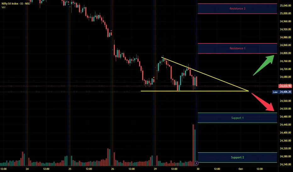
Nifty Intraday Analysis for 30th September 2025NSE:NIFTY
Index has resistance near 24800 – 24850 range and if index crosses and sustains above this level then may reach near 25000 – 25050 range.
Nifty has immediate support near 24500 – 24450 range and if this support is broken then index may tank near 24300 – 24250 range.
The market may move in the direction where unwinding of OI takes place on the Monthly F&O expiry day. Volatility expected.
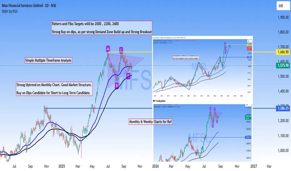
MFSL Multi time frame AnalysisMulti-timeframe confluence analysis offers traders a robust edge through straightforward yet highly effective methodology.
Based on that MFSL is a strong Buy on dips stock based on powerful breakout of previous ATH and the current market structure.
Targets are derived from #Pattern #breakout and #Fibonacci levels.
Bullish Pennant in formation.
Disclaimer: Above analysis shared for educational purpose only.
Bitcoin – Let’s Play the Resistance Game at 114,500Bitcoin on the 1-hour chart has entered a critical resistance zone around 114,200–114,500. Price has rallied strongly from the recent lows near 113,000, but now faces a major supply area. The structure suggests that BTC could face rejection here and move back toward the support zone near 112,600 if sellers step in.
As long as price stays below 114,500, this resistance remains valid. A clean breakout above this level with strong momentum would invalidate the bearish view and open the path for higher levels. On the downside, holding support near 112,600 will be key for buyers to maintain control.
Disclaimer: This analysis is for educational purposes only and should not be taken as financial advice. Please do your own research or consult your financial advisor before investing.
Analysis By @TraderRahulPal (TradingView Moderator) | More analysis & educational content on my profile
👉 If you found this helpful, don’t forget to like and follow for regular updates.

Part 1 Ride The Big Moves1. Introduction to Options
An option is a financial contract that gives the buyer the right, but not the obligation, to buy or sell an underlying asset at a predetermined price, called the strike price, before or on a specified expiration date. Unlike stocks, options do not represent ownership in a company; instead, they are derivatives whose value is derived from the underlying asset (stocks, indices, commodities, or currencies).
There are two primary types of options:
Call Option: Grants the holder the right to buy the underlying asset at the strike price.
Put Option: Grants the holder the right to sell the underlying asset at the strike price.
Options can be American style (exercisable any time before expiration) or European style (exercisable only on the expiration date).
2. Key Terminology in Options Trading
To trade options effectively, you must understand the key terms:
Strike Price (Exercise Price): The price at which the underlying asset can be bought (call) or sold (put).
Premium: The cost of buying an option. Determined by factors like intrinsic value, time to expiration, volatility, and interest rates.
Expiration Date: The date on which the option contract becomes invalid.
In-the-Money (ITM): A call option is ITM if the stock price > strike price; a put is ITM if stock price < strike price.
Out-of-the-Money (OTM): A call option is OTM if the stock price < strike price; a put is OTM if stock price > strike price.
At-the-Money (ATM): The stock price is approximately equal to the strike price.
3. How Options Work
Options allow investors to control a larger number of shares with relatively small capital. Let’s look at an example:
Example:
Stock price of XYZ Ltd.: ₹1,000
Call option strike price: ₹1,050
Premium: ₹50
Expiration: 1 month
If the stock rises to ₹1,200, the call option holder can exercise the option, buy at ₹1,050, and sell at ₹1,200, making a profit of ₹150 per share (minus the premium of ₹50, net profit = ₹100).
If the stock stays below ₹1,050, the option expires worthless, and the loss is limited to the premium paid.
This limited-loss feature makes options attractive for hedging.
4. Participants in Options Market
Options trading involves different market participants with varying objectives:
Hedgers: Use options to protect their existing investments from adverse price movements. For example, a stock investor buys a put option to safeguard against a potential fall in stock price.
Speculators: Seek profit from price movements without owning the underlying asset. They take higher risk for potentially higher rewards.
Arbitrageurs: Exploit price discrepancies between options and the underlying assets to earn risk-free profits.
5. Option Pricing Models
Option pricing is critical for traders. The two most commonly used models are:
Black-Scholes Model (for European options):
It calculates the theoretical value of options using factors such as stock price, strike price, time to expiration, volatility, and risk-free interest rate.
Binomial Model:
Uses a step-by-step approach to evaluate options, useful for American options due to their early-exercise feature.
Factors Affecting Option Premiums:
Intrinsic Value: Difference between the underlying price and strike price.
Time Value: Additional value due to remaining time until expiration.
Volatility: Higher volatility increases premiums.
Interest Rates and Dividends: Can influence option pricing.

Part 11 Trading Master Class With ExpertsI. Option Trading Strategies
Buying Calls and Puts
Buying a Call: Profitable if asset price rises above strike + premium.
Buying a Put: Profitable if asset price falls below strike - premium.
Covered Call Strategy
Involves holding the underlying stock and selling a call option.
Generates premium income but limits upside profit.
Protective Put
Buying a put while holding the underlying asset as insurance against a price drop.
Spreads
Combine buying and selling options to reduce risk and cost:
Bull Call Spread: Buy lower strike call, sell higher strike call.
Bear Put Spread: Buy higher strike put, sell lower strike put
Straddles and Strangles
Straddle: Buy ATM call and put; profitable if price moves significantly either way.
Strangle: Buy OTM call and put; cheaper than straddle, requires larger movement.
Iron Condor
Advanced strategy combining bull and bear spreads.
Generates income with limited risk in low-volatility markets.
Calendar and Diagonal Spreads
Utilize different expiration dates and strikes to profit from time decay and volatility.
II. Risk Management in Options
Leverage and Risk
Options offer high leverage: small price moves in underlying asset can lead to large gains or losses. Proper position sizing is crucial.
Maximum Loss and Gain
Buyer: Max loss = premium paid; Max gain = theoretically unlimited for calls, limited for puts.
Seller: Max gain = premium received; Max loss = potentially unlimited for naked calls.
Diversification Across Strategies
Mixing spreads, covered calls, and protective puts helps reduce single-position risk.
Stop-Loss and Exit Strategies
Plan exit points: cut losses, take partial profits, or roll positions to new strikes or expirations.
III. Market Mechanics and Trading
Exchanges and Option Contracts
Options trade on regulated exchanges (e.g., NSE, BSE, CBOE). Each contract represents a fixed quantity of the underlying (e.g., 100 shares per contract).
Liquidity and Open Interest
Liquidity: Ease of buying/selling options at fair prices.
Open Interest: Number of outstanding contracts; higher OI often means better liquidity.
Implied Volatility and Market Sentiment
IV: Market’s forecast of future volatility.
Rising IV generally increases option premiums, signaling uncertainty.
Hedging vs. Speculation
Options can hedge existing positions or speculate on market movements. Hedging reduces risk, speculation increases risk but offers leverage.

Part 12 Trading Master Class With ExpertsI. Introduction to Options
What is an Option?
An option is a financial derivative contract that gives the buyer the right, but not the obligation, to buy or sell an underlying asset at a predetermined price (strike price) within a specified time period. Options derive their value from the underlying asset, which can be stocks, indices, commodities, currencies, or ETFs.
Types of Options
There are two primary types:
Call Option: Gives the holder the right to buy the underlying asset at a strike price before expiration.
Put Option: Gives the holder the right to sell the underlying asset at a strike price before expiration.
Buyers vs. Sellers
Option Buyer (Holder): Pays a premium for the right to exercise the option. Limited risk (premium paid), unlimited or capped potential reward depending on call or put.
Option Seller (Writer): Receives the premium. Obligated to fulfill the contract if exercised. Higher risk, especially in uncovered options.
Option Premium Explained
The premium is the price paid for the option. It comprises two components:
Intrinsic Value: The real, immediate profit if exercised now (for in-the-money options).
Time Value: Additional value based on time left until expiration and market volatility.
Option Expiration and Exercise
Options have a fixed expiration date. Exercise can happen in two ways:
American Style: Can be exercised any time before expiration.
European Style: Can only be exercised at expiration.
II. Understanding Option Pricing
Factors Affecting Option Pricing
The price of an option (premium) is influenced by:
Underlying asset price
Strike price
Time to expiration
Volatility
Interest rates
Dividends
Intrinsic vs. Extrinsic Value
Intrinsic Value: Difference between underlying asset price and strike price (only if in-the-money).
Extrinsic Value: Time value and volatility premium. Represents potential for future gains.
Moneyness of Options
Options are classified based on their intrinsic value:
In-the-Money (ITM): Profitable if exercised now.
At-the-Money (ATM): Strike price equals the underlying asset price.
Out-of-the-Money (OTM): Not profitable if exercised now.
The Greeks – Risk and Sensitivity Measures
Options are influenced by “Greeks” which measure sensitivity to different factors:
Delta: Sensitivity of option price to underlying asset price change.
Gamma: Rate of change of delta.
Theta: Time decay of option value.
Vega: Sensitivity to volatility.
Rho: Sensitivity to interest rates.
Black-Scholes & Binomial Models
Option pricing models estimate theoretical values:
Black-Scholes Model: For European options; factors in price, strike, volatility, time, and risk-free rate.
Binomial Model: Uses a stepwise approach; suitable for American options.

Gold 30/09 - Safe-haven flows surge | Gold sails toward new ATH 🟡 XAU/USD – 30/09 | Captain Vincent ⚓
🔎 Captain’s Log – Context & News
US Politics : Meeting between Trump and bipartisan leaders ended without agreement → growing risk of a US government shutdown by Wednesday.
Conflict : Democrats demand concessions, Republicans fiercely oppose → wide gap remains, both sides blaming each other.
Market : Investors watch JOLTS data and speeches from 3 FED members, but political risks are the strongest catalyst for Gold.
Trend : Safe-haven flows keep pouring into Gold → increasing likelihood of testing new ATH.
⏩ Captain’s Summary : US political seas are stormy, Gold becomes the fortress of safety. The voyage toward ATH is widening.
📈 Captain’s Chart – Technical Analysis (H1)
EMA : EMA 34 (yellow) > EMA 89 (red) → bullish trend clearly dominant.
Golden Harbor (Support / Buy Zone)
Big Volume Dock: 3,827
Storm Breaker (Resistance / Sell Zone)
ATH test: 3,916 – 3,917
Market Structure : Gold broke out strongly, now trading around 3,870. Main trend remains bullish, with 3,842 – 3,827 as key anchor zones.
🎯 Captain’s Map – Trade Plan
✅ Buy (main priority)
Buy Zone 2 – Big Volume
Entry: 3,827 – 3,824
SL: 3,815
TP: 3,870 – 3,899 – 3,916
⚡ Sell (short scalp – high risk)
Sell Zone – ATH test
Entry: 3,917 – 3,920
SL: 3,925
TP: 3,899 – 3,870 – 3,856
⚓ Captain’s Note
“The Golden sails are filled by safe-haven winds, pushing the ship close to ATH. Golden Harbor 🏝️ (3,842 – 3,827) is the ideal dock for sailors to position Buys. Storm Breaker 🌊 (3,916 – 3,920) may unleash violent waves, suitable only for short Quick Boarding 🚤 scalps. If the political storm from Washington breaks out, Gold’s voyage could surpass the peak and expand its horizon.”
📢 If you find the Captain’s Log useful, don’t forget to Follow for the earliest updates.
💬 What’s your view, crew? Will Gold conquer ATH around 3,917 this week?

OLA looks good for higher levelsLooks like OLA has started rising from the ashes... SL near 46 may be a good idea where maximum volumes hv happened.

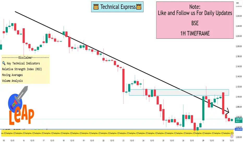
BSE 1 Hour ViewBSE is trading at ₹2,054.60, reflecting a 2.04% decline for the day.
📊 1-Hour Time Frame Technical Analysis
On the 1-hour chart, BSE Ltd. is exhibiting a "Strong Sell" signal across both technical indicators and moving averages. This suggests a prevailing short-term downtrend, with the stock trading below its key moving averages.
🔍 Key Technical Indicators
Relative Strength Index (RSI): Currently below 30, indicating the stock is in oversold territory and may be due for a short-term rebound.
Moving Averages: The stock is trading below its 5-day, 20-day, 50-day, 100-day, and 200-day moving averages, suggesting a bearish trend.
Volume Analysis: Recent trading volumes have been lower than average, indicating reduced investor participation.
📈 Support and Resistance Levels
Immediate Support: ₹2,000
Immediate Resistance: ₹2,100
A break below ₹2,000 could signal further downside, while a move above ₹2,100 may indicate a potential reversal.
⚠️ Considerations for Traders
Given the current "Strong Sell" signals, traders should exercise caution. It's advisable to wait for confirmation of a trend reversal before entering long positions. Utilizing a multi-timeframe analysis can provide a more comprehensive view of the stock's potential movements.
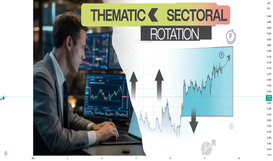
Thematic and Sectoral Rotation Trading1. Introduction
In financial markets, investors and traders are continuously seeking methods to maximize returns while managing risk. Among the myriad strategies, thematic and sectoral rotation trading has gained immense popularity because it aligns investment decisions with evolving economic trends, technological advancements, and market cycles. Unlike traditional strategies that might focus purely on individual securities, sectoral and thematic approaches leverage broader economic patterns, industry performance, and market sentiment.
At its core, sectoral rotation involves shifting capital from one industry sector to another based on their performance in different phases of the economic cycle. Thematic trading, meanwhile, focuses on investing in specific themes or trends, such as renewable energy, digitalization, or electric vehicles, which have potential long-term growth driven by structural shifts in society and the economy.
Understanding these strategies requires a deep dive into economic cycles, market behavior, sector dynamics, and thematic trends.
2. Concept of Sectoral Rotation Trading
2.1 Definition
Sectoral rotation trading is a strategy where investors systematically move investments between sectors to capitalize on varying performances of sectors during different phases of the economic cycle.
2.2 Rationale
Different sectors perform differently depending on macroeconomic conditions. For example:
Early economic recovery: Cyclical sectors like consumer discretionary and technology often lead.
Economic expansion: Industrial and capital goods sectors see strong growth.
Late-stage expansion: Defensive sectors like healthcare, utilities, and consumer staples tend to outperform.
Recession: Safe-haven sectors such as utilities and healthcare gain attention due to lower volatility.
This rotation is based on the understanding that capital flows dynamically between sectors to optimize returns based on economic conditions.
2.3 Sector Classification
Sectors are typically classified into:
Cyclical sectors: Highly sensitive to economic cycles (e.g., consumer discretionary, industrials, technology).
Defensive sectors: Less sensitive to economic cycles (e.g., utilities, healthcare, consumer staples).
Financial sectors: Banks and insurance, which are influenced by interest rate policies.
Commodity sectors: Energy, materials, metals, and mining.
3. Concept of Thematic Trading
3.1 Definition
Thematic trading is investing in broader trends or megatrends that transcend individual sectors. Unlike sectoral trading, themes are based on structural changes in society, technology, or regulations, rather than the economic cycle alone.
3.2 Examples of Themes
Some of the most prominent themes include:
Renewable Energy: Solar, wind, and battery storage companies.
Electric Vehicles (EVs): EV manufacturers, battery producers, and charging infrastructure.
Artificial Intelligence (AI) & Automation: AI software, robotics, and automation solutions.
Healthcare Innovation: Biotech, genomics, telemedicine.
Digital Transformation: Cloud computing, cybersecurity, e-commerce platforms.
3.3 Advantages
Exposure to long-term structural growth.
Diversification beyond traditional sector boundaries.
Ability to capitalize on global megatrends.
4. Key Differences Between Sectoral and Thematic Trading
Feature Sectoral Rotation Trading Thematic Trading
Basis Economic cycles and sector performance Structural trends or megatrends
Time Horizon Medium-term to short-term Medium-term to long-term
Focus Sector performance Specific themes cutting across sectors
Risk Profile Moderately lower if diversified across sectors Can be higher due to concentration in themes
Performance Drivers GDP growth, interest rates, inflation Technological innovation, regulatory changes, societal shifts
Examples Shifting from energy to technology during recovery Investing in EV and renewable energy stocks
5. Economic Cycle and Sector Rotation
The sectoral rotation strategy is closely tied to the economic cycle, which can be divided into four phases:
5.1 Early Recovery
Characteristics: Low interest rates, improving GDP, rising consumer confidence.
Outperforming sectors: Cyclical sectors like consumer discretionary, technology, and industrials.
Trading strategy: Rotate capital from defensive sectors to high-growth cyclical sectors.
5.2 Economic Expansion
Characteristics: High consumer spending, rising corporate profits.
Outperforming sectors: Industrials, financials, materials.
Trading strategy: Increase exposure to sectors benefiting from rising demand and investments.
5.3 Late-Stage Expansion
Characteristics: Slowing growth, inflation concerns, peak corporate earnings.
Outperforming sectors: Defensive sectors such as healthcare, utilities, and consumer staples.
Trading strategy: Shift from high-risk cyclical sectors to low-volatility defensive sectors.
5.4 Recession
Characteristics: Declining GDP, falling corporate profits, rising unemployment.
Outperforming sectors: Utilities, healthcare, consumer staples (defensive sectors).
Trading strategy: Reduce exposure to cyclical sectors and allocate to defensive sectors for capital preservation.
6. Key Indicators for Sectoral Rotation
Traders often use a combination of macro indicators, technical analysis, and sector-specific metrics to guide rotation strategies.
6.1 Economic Indicators
GDP growth
Inflation rate
Interest rates
Consumer confidence
Industrial production
6.2 Market Indicators
Relative strength of sector indices
Sector ETF flows
Price-to-earnings (P/E) ratios
Moving averages and technical trends
6.3 Sector-Specific Metrics
Financials: Net interest margin, credit growth
Technology: Revenue growth, R&D expenditure
Energy: Oil prices, renewable capacity growth
Consumer: Retail sales, brand performance
7. Tools and Instruments for Sectoral Rotation
Sectoral rotation strategies can be executed through multiple instruments:
Sector ETFs: Exchange-Traded Funds representing specific sectors (e.g., technology, healthcare).
Mutual Funds: Sector-specific funds for active management.
Stocks: Direct investment in companies leading their respective sectors.
Options and Futures: Derivatives to hedge or leverage sector exposure.
8. Advantages of Sectoral Rotation Trading
Optimized Returns: Capitalizes on outperforming sectors during different phases.
Diversification: Reduces risk by not being tied to a single sector.
Tactical Flexibility: Can adjust quickly to macroeconomic changes.
Evidence-Based: Relies on historical patterns of sector performance.
9. Risks of Sectoral Rotation Trading
Timing Risk: Misjudging the start or end of a sector’s cycle can lead to losses.
Concentration Risk: Overweighting a sector exposes the portfolio to sector-specific downturns.
Market Volatility: Rapid market changes can disrupt rotation strategy.
Transaction Costs: Frequent trading may increase costs, reducing net returns.
10. Conclusion
Thematic and sectoral rotation trading is a powerful approach to optimizing returns by leveraging macroeconomic cycles and long-term structural trends. While sectoral rotation aligns with the economic phases to identify cyclical and defensive opportunities, thematic trading focuses on long-term megatrends that cut across sectors and markets.
Both strategies require:
Thorough research
Economic and market analysis
Risk management
When implemented correctly, these approaches can help traders and investors maximize growth, diversify risk, and stay ahead of market trends. Integrating sectoral and thematic approaches provides a robust portfolio strategy that captures cyclical performance while riding long-term structural growth trends.
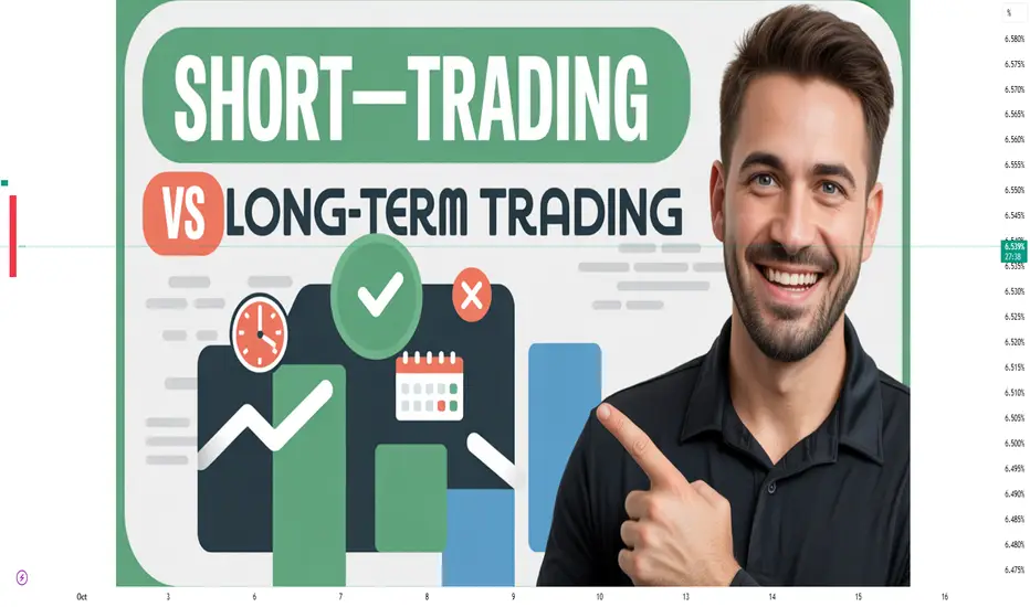
Short-Term Trading vs Long-Term Trading1. Introduction
Financial markets offer multiple avenues for wealth creation. From stocks, commodities, and currencies to derivatives and bonds, the market landscape is diverse. Two primary approaches dominate this landscape:
Short-Term Trading (STT): Trading where positions are held for hours, days, or weeks.
Long-Term Trading (LTT): Investing where positions are held for months, years, or even decades.
Choosing between these approaches is not merely a matter of preference; it involves evaluating capital availability, risk tolerance, skill level, and desired outcomes.
2. Short-Term Trading
2.1 Definition
Short-term trading refers to buying and selling financial instruments over a brief period to capitalize on price fluctuations. The goal is to profit from market volatility, irrespective of long-term market trends.
2.2 Types of Short-Term Trading
Intraday Trading:
Positions are opened and closed within the same trading day.
No overnight risk is taken.
Traders rely heavily on technical analysis, charts, and indicators.
Swing Trading:
Trades last from a few days to several weeks.
Aims to capture price swings within an intermediate trend.
Combines technical and fundamental analysis.
Scalping:
Ultra-short-term trading, often holding positions for minutes or seconds.
Focuses on micro price movements and liquidity.
2.3 Key Features of Short-Term Trading
Time Horizon: Minutes to weeks.
Analysis Tools: Technical analysis dominates; charts, volume, momentum, moving averages.
Capital Requirements: Moderate to high, depending on leverage and trade frequency.
Risk Level: High; price volatility can lead to substantial gains or losses.
Psychological Demands: High stress; requires constant monitoring and quick decision-making.
Transaction Costs: Frequent trades increase brokerage and taxes.
2.4 Advantages of Short-Term Trading
Quick capital turnover.
Multiple profit opportunities in volatile markets.
Ability to exploit technical market inefficiencies.
Flexibility to adjust positions rapidly.
2.5 Disadvantages of Short-Term Trading
High stress and emotional pressure.
Requires significant time commitment.
Transaction costs can erode profits.
High risk of losses during unexpected market events.
2.6 Strategies in Short-Term Trading
Trend Following: Riding the market trend until a reversal signal appears.
Counter-Trend: Betting against the current trend for short-term correction profits.
Breakout Trading: Entering trades when price breaks support or resistance levels.
Momentum Trading: Using indicators like RSI or MACD to capture strong price movements.
3. Long-Term Trading
3.1 Definition
Long-term trading, or investing, involves holding positions over extended periods, ranging from months to years, focusing on the fundamental value of an asset rather than short-term price fluctuations.
3.2 Types of Long-Term Trading
Position Trading:
Holding trades for months to years.
Focused on macroeconomic trends, corporate fundamentals, and industry growth.
Value Investing:
Buying undervalued stocks and holding until the market recognizes their true value.
Popularized by investors like Warren Buffett.
Dividend Investing:
Focused on income generation through dividends alongside capital appreciation.
3.3 Key Features of Long-Term Trading
Time Horizon: Months to decades.
Analysis Tools: Fundamental analysis dominates; financial statements, P/E ratios, cash flows.
Capital Requirements: Can start small but often requires patience to realize returns.
Risk Level: Generally lower; time helps smooth out market volatility.
Psychological Demands: Patience and discipline are essential; minimal day-to-day stress.
Transaction Costs: Lower due to fewer trades.
3.4 Advantages of Long-Term Trading
Benefits from compounding over time.
Less stress compared to short-term trading.
Lower transaction costs.
Less impacted by daily market volatility.
3.5 Disadvantages of Long-Term Trading
Requires patience and discipline.
Capital is tied up for longer periods.
Market shocks (e.g., recessions, policy changes) can affect returns temporarily.
3.6 Strategies in Long-Term Trading
Buy and Hold: Purchase quality assets and hold for long periods.
Dollar-Cost Averaging: Investing a fixed amount regularly to mitigate timing risks.
Growth Investing: Targeting companies with strong future growth potential.
Index Fund Investing: Diversifying risk through market indices like S&P 500 or Nifty 50.
4. Risk Management
Both approaches require risk management:
4.1 Short-Term Risk Management
Stop-loss orders to limit losses.
Position sizing based on volatility.
Diversifying trades to reduce market dependency.
Avoiding over-leverage.
4.2 Long-Term Risk Management
Portfolio diversification across sectors and assets.
Regularly reviewing fundamentals.
Maintaining emergency funds to avoid forced liquidation.
Hedging with derivatives or protective instruments if necessary.
5. Psychological Considerations
5.1 Short-Term Trading Psychology
Emotional control is critical; impulsive decisions can cause losses.
Fear and greed dominate daily trading.
Traders must develop a clear strategy and stick to it.
5.2 Long-Term Trading Psychology
Patience and resilience are key.
Avoid reacting to market noise.
Focus on long-term goals rather than short-term market movements.
6. Tools and Technology
Both trading types benefit from modern technology:
Short-Term Traders: Charting software, trading platforms, algorithmic tools, high-speed data feeds.
Long-Term Traders: Research platforms, financial news, fundamental databases, portfolio trackers.
7. Tax Implications
Taxation varies by country and can influence trading strategies:
Short-Term Trading: Usually taxed at higher rates as short-term capital gains.
Long-Term Trading: Often enjoys lower tax rates on long-term capital gains.
8. Case Studies
8.1 Short-Term Trading Example
Day trader using RSI and MACD indicators to trade Nifty futures within a single day.
Captures profit of 0.5%-1% per trade but executes 10-15 trades per week.
8.2 Long-Term Trading Example
Investor buys shares of a growing IT company and holds for 5 years.
Benefits from dividends and capital appreciation as the company expands.
Conclusion
Short-term and long-term trading represent different philosophies of engaging with the financial markets:
Short-Term Trading is action-oriented, volatile, and requires skill, discipline, and constant attention.
Long-Term Trading is patience-oriented, fundamentally driven, and benefits from compounding over time.
A comprehensive understanding of both allows traders to design a strategy that balances risk, reward, and personal lifestyle, ensuring sustainable financial growth in dynamic markets.
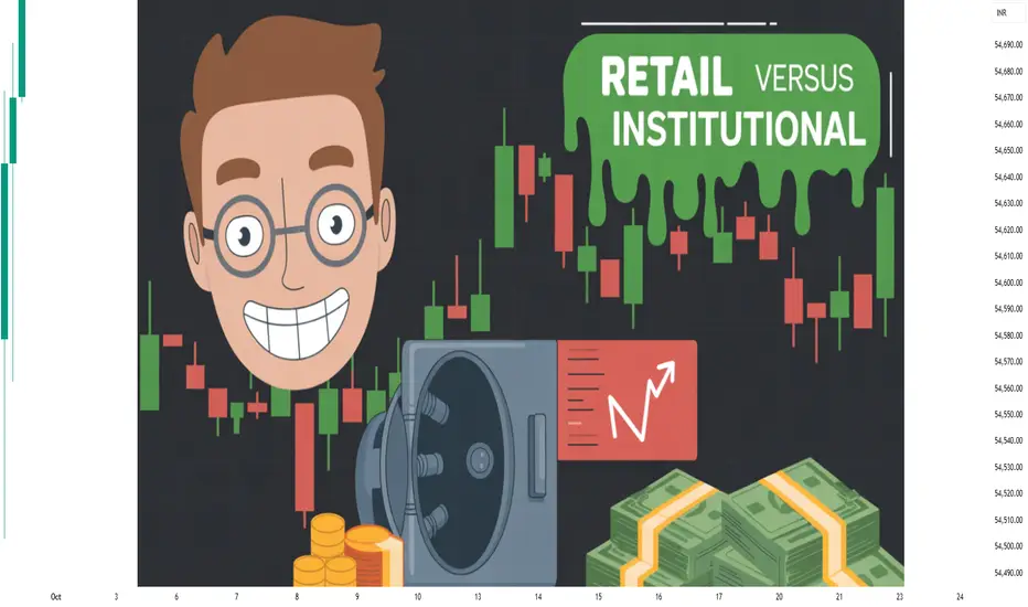
Retail vs Institutional Trading1. Introduction to Trading Participants
1.1 Retail Traders
Retail traders, often referred to as individual investors, are non-professional participants in financial markets. They trade personal funds rather than pooled or client capital. Retail traders can include anyone from a small investor buying a few shares in the stock market to active traders participating in forex, commodities, or cryptocurrency markets.
Key Characteristics:
Trade smaller volumes compared to institutions.
Decisions are often influenced by news, social media, market sentiment, or personal beliefs.
Typically have limited access to advanced tools and institutional-grade research.
1.2 Institutional Traders
Institutional traders represent organizations managing large sums of money, including mutual funds, hedge funds, pension funds, insurance companies, banks, and investment firms. They trade on behalf of clients or institutional portfolios and often have significant influence on market prices due to their trade volumes.
Key Characteristics:
Trade in large volumes, often moving markets.
Utilize professional research, proprietary trading algorithms, and sophisticated analytics.
Longer-term investment horizons, though some engage in high-frequency trading.
2. Market Participation and Influence
2.1 Retail Participation
Retail traders historically had limited influence in the markets due to smaller trade sizes. However, the rise of online trading platforms, zero-commission trading, and social media-driven movements (e.g., meme stocks) has increased retail impact in recent years.
Advantages of Retail Participation:
Flexibility to react quickly.
Ability to pursue niche opportunities or speculative trades.
Lower regulatory burdens allow creative strategies.
Disadvantages:
Susceptibility to emotional trading.
Higher vulnerability to market manipulation.
Limited access to professional research and tools.
2.2 Institutional Participation
Institutional traders dominate market liquidity and pricing. Their large trades can move market prices, create trends, or influence volatility. They are also instrumental in market stability as they provide liquidity during periods of stress.
Advantages of Institutional Trading:
Access to advanced market intelligence and professional research.
Ability to use sophisticated trading strategies, including algorithmic trading.
Can leverage economies of scale for reduced transaction costs.
Disadvantages:
Large trades may impact markets in ways that reduce profitability.
Regulatory scrutiny is stringent, limiting flexibility.
Requires complex risk management due to large exposure.
3. Trading Strategies
3.1 Retail Trading Strategies
Retail traders often employ strategies based on technical analysis, short-term news, or trend-following techniques.
Popular Strategies:
Day Trading: Buying and selling securities within the same trading day.
Swing Trading: Holding positions for several days to capture short-term market movements.
Momentum Trading: Riding price trends based on market sentiment.
News Trading: Reacting to economic reports, corporate earnings, or geopolitical events.
3.2 Institutional Trading Strategies
Institutional traders adopt more sophisticated strategies due to their large capital base and professional resources.
Popular Strategies:
Algorithmic Trading (Algo-Trading): Using computer programs to execute trades at optimal prices.
High-Frequency Trading (HFT): Executing thousands of trades in milliseconds to exploit small market inefficiencies.
Arbitrage: Taking advantage of price differences across markets.
Hedging and Risk Management: Using derivatives to manage exposure to currency, interest rate, or market risk.
4. Risk Management
4.1 Retail Risk Management
Retail traders often rely on basic risk management tools such as:
Stop-loss orders.
Position sizing based on personal risk tolerance.
Diversification across a few stocks or sectors.
However, retail investors are prone to emotional decisions, such as holding losing positions too long or chasing returns impulsively.
4.2 Institutional Risk Management
Institutions adopt structured risk frameworks, including:
Value-at-Risk (VaR): Quantifying potential losses under normal market conditions.
Stress Testing: Evaluating portfolio performance under extreme scenarios.
Diversification and Hedging: Using derivatives, multiple asset classes, and global exposure to mitigate risk.
Regulatory Compliance: Ensuring all trades adhere to legal and fiduciary requirements.
5. Technology and Tools
5.1 Retail Technology
Retail traders have benefited from:
Online trading platforms like Zerodha, Robinhood, and E*TRADE.
Mobile apps for instant trading and market tracking.
Charting tools for technical analysis (TradingView, MetaTrader).
5.2 Institutional Technology
Institutions use highly advanced tools:
Proprietary trading algorithms with AI and machine learning.
Direct market access (DMA) platforms for faster execution.
Risk analytics software for real-time portfolio monitoring.
Big data analytics for predictive market insights.
6. Regulatory Environment
6.1 Retail Trading Regulations
Retail traders are primarily regulated to ensure transparency and protect against fraud:
Know Your Customer (KYC) requirements.
Disclosure of fees and commissions.
Restrictions on certain high-risk products without adequate knowledge.
6.2 Institutional Trading Regulations
Institutional traders face stricter oversight:
Reporting large trades and positions.
Compliance with investment mandates.
Adherence to market conduct rules and fiduciary duties.
Stress testing for systemic risk management.
7. Psychology and Behavioral Differences
7.1 Retail Trader Psychology
Retail traders are heavily influenced by emotion:
Fear and Greed: Leading to panic selling or impulsive buying.
Overconfidence: Believing in personal market insight without adequate data.
Herd Mentality: Following trends or social media-driven movements.
7.2 Institutional Trader Psychology
Institutional traders operate under disciplined frameworks:
Decisions are data-driven and analytical.
Emotional biases are minimized through systematic strategies.
Portfolio-level focus reduces reactionary decisions.
8. Conclusion
The contrast between retail and institutional trading illustrates the diversity of market participants. Retail traders bring flexibility, innovation, and sentiment-driven momentum, while institutions contribute liquidity, stability, and analytical rigor. Both are essential for a healthy financial ecosystem.
Understanding their differences, behaviors, and strategies allows traders to navigate markets more effectively, whether by learning from institutional methodologies or leveraging the unique advantages of retail agility. In today’s technology-driven world, the line between retail and institutional trading is increasingly blurred, creating a dynamic and evolving marketplace where knowledge, strategy, and discipline define success.
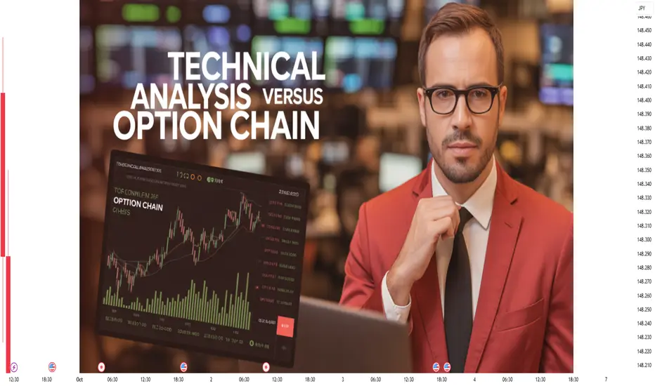
Technical Analysis vs. Option Chain Analysis in Trading1. Introduction to Technical Analysis
Technical Analysis is the study of historical price and volume data to forecast future price movements. Unlike fundamental analysis, which focuses on the intrinsic value of an asset based on financials and macroeconomic indicators, technical analysis relies solely on market data.
Core Principles of Technical Analysis:
Price Discounts Everything:
TA assumes that all known information (fundamental, political, economic) is already reflected in the price. Therefore, price movements are sufficient for forecasting future trends.
Price Moves in Trends:
Markets rarely move randomly. They exhibit trends—uptrend, downtrend, or sideways—which traders identify and trade accordingly.
History Repeats Itself:
Market behavior tends to repeat due to human psychology, making chart patterns, technical indicators, and market cycles predictive.
Key Tools in Technical Analysis:
Charts: Line charts, bar charts, candlestick charts
Indicators: RSI, MACD, Bollinger Bands, moving averages
Patterns: Head & shoulders, double top/bottom, triangles
Volume Analysis: Confirms trends and reversals
Practical Applications:
Identifying entry and exit points
Spotting trends and reversals
Risk management using support, resistance, and stop-loss
Advantages of Technical Analysis:
Works in all market conditions
Can be automated using algorithmic trading
Useful for both short-term and long-term trading
Limitations:
Subjective interpretation of charts
Can give false signals in volatile markets
Does not consider underlying fundamentals
2. Introduction to Option Chain Analysis
Option Chain Analysis involves examining the details of options contracts available for a particular stock or index. An option chain lists all available options (calls and puts) along with their strike prices, premiums, open interest (OI), and volume.
Unlike technical analysis, option chain analysis is specific to derivatives and is used to infer market sentiment and potential price movements.
Core Concepts of Option Chain Analysis:
Calls and Puts:
Call Option: Right to buy at a specific price
Put Option: Right to sell at a specific price
Strike Price: The price at which the underlying asset can be bought or sold.
Open Interest (OI): Number of outstanding contracts. High OI at specific strikes can indicate support or resistance zones.
Volume: Number of contracts traded in a day, indicating trader interest.
Implied Volatility (IV): Market’s forecast of volatility, impacting option premiums.
Key Applications of Option Chain Analysis:
Identifying support and resistance levels using maximum OI strikes
Predicting short-term price movements based on put-call ratios (PCR)
Planning hedging strategies using options
Understanding market sentiment
Advantages:
Provides real-time insight into market sentiment
Useful for short-term trading and intraday strategies
Helps in planning hedging strategies for portfolios
Limitations:
Requires understanding of options pricing
Complex for beginners
Influenced by external factors like volatility and time decay
3. Technical Analysis in Depth
3.1 Price Action
Price action refers to the movement of price over time.
Candlestick patterns (Doji, Hammer, Engulfing) help identify reversals and continuations.
Trendlines and channels assist in visualizing the market direction.
3.2 Indicators and Oscillators
Moving Averages: Smooth out price data; 50-day & 200-day MAs show trend strength.
MACD (Moving Average Convergence Divergence): Shows momentum and trend changes.
RSI (Relative Strength Index): Identifies overbought/oversold conditions.
Bollinger Bands: Measures volatility; price touching bands signals potential reversal.
3.3 Volume Analysis
Volume confirms trend strength.
Rising price with high volume = strong trend; Falling price with high volume = potential reversal.
3.4 Chart Patterns
Reversal Patterns: Head & Shoulders, Double Top/Bottom
Continuation Patterns: Triangles, Flags, Pennants
4. Option Chain Analysis in Depth
4.1 Understanding Option Data
Calls vs Puts: Analyzing the ratio helps gauge bullish or bearish sentiment.
Open Interest (OI): Strikes with high OI act as psychological support/resistance.
Volume: High trading volume at a strike indicates trader focus.
4.2 Put-Call Ratio (PCR)
PCR = Total Put OI / Total Call OI
PCR > 1 indicates bearish sentiment; PCR < 1 indicates bullish sentiment.
4.3 Max Pain Theory
Max Pain = strike where option writers lose the least money
Price tends to gravitate towards max pain level near expiry
4.4 Implied Volatility (IV)
High IV = expensive options, often during high uncertainty
Low IV = cheap options, during stable periods
Helps in timing entry and exit points in options trading
5. Integrating Technical and Option Chain Analysis
Successful traders often combine both approaches:
Confirming Trend with TA and OCA:
Technical indicators may show uptrend.
Option chain OI analysis confirms resistance/support levels, giving high-probability entry points.
Hedging Positions:
Buy stock based on TA trend.
Hedge using options with OCA support.
Intraday Trading:
Use TA for momentum and pattern breakout.
Use OCA for strike-based resistance and price targets.
Volatility Trading:
Use TA to identify consolidation or breakout zones.
Use OCA IV data to choose options strategies (straddle, strangle).
6. Case Study Example
Stock: XYZ Ltd.
TA Observation: 50-day MA trending upward, RSI around 65 → bullish bias
Option Chain Analysis:
Max Call OI at 150 strike → strong resistance
Max Put OI at 140 strike → strong support
PCR = 0.8 → bullish sentiment
Trading Strategy:
Enter long near support (140)
Target price near resistance (150)
Use options to hedge if breakout fails
7. Pros and Cons in Trading Context
7.1 Technical Analysis Pros and Cons
Pros:
Easy to interpret
Widely applicable
Works across timeframes
Cons:
Cannot measure market sentiment directly
False breakouts possible
Subjective
7.2 Option Chain Analysis Pros and Cons
Pros:
Reveals trader sentiment
Helps with hedging
Useful for expiry-week trading
Cons:
Complex interpretation
Affected by volatility and time decay
Requires options knowledge
8. Conclusion
Both Technical Analysis and Option Chain Analysis are indispensable tools for traders. While TA provides a structured approach to reading price trends and patterns, OCA adds depth by revealing market sentiment and strike-based support/resistance. Combining both approaches gives traders a holistic view, enabling better risk management, precise entry/exit points, and a strategic edge in the market.
TA: Broadly applicable, trend and pattern-based, foundational for all traders.
OCA: Derivatives-focused, sentiment-driven, crucial for options and intraday trading.
Combined Approach: Confirms technical signals, improves probability of success, and optimizes risk management.
For modern traders, understanding both TA and OCA is no longer optional—it is essential to navigate volatile markets and enhance decision-making capabilities.
Intraday and Swing Trading1. Intraday Trading
1.1 Definition
Intraday trading is the practice of buying and selling securities within a single trading day. Traders aim to profit from short-term price fluctuations and must close all positions before the market closes. The key feature of intraday trading is its very short time frame, which can range from a few minutes to several hours within the same day.
1.2 Objectives of Intraday Trading
Profit from Volatility: Intraday traders capitalize on small price movements and volatility within the day.
Avoid Overnight Risk: By closing positions before the market closes, traders avoid risks associated with overnight events like news releases, economic announcements, or geopolitical developments.
Liquidity Utilization: Intraday traders prefer highly liquid stocks and indices to ensure easy entry and exit at favorable prices.
1.3 Key Characteristics
Short Time Horizon: Trades last minutes to hours, rarely overnight.
High Frequency: Traders often execute multiple trades in a single day.
Leverage Usage: Intraday trading often involves leverage to amplify returns, increasing both potential gains and risks.
Technical Analysis Oriented: Decisions rely heavily on charts, patterns, and indicators rather than fundamental analysis.
Rapid Decision-Making: Traders must react quickly to market movements to avoid losses.
1.4 Tools and Techniques
Intraday trading relies heavily on technical analysis, which includes chart patterns, technical indicators, and market data. Key tools include:
Candlestick Charts: Provide visual representation of price movements and patterns like Doji, Hammer, or Engulfing patterns.
Moving Averages (MA): Help identify trends and dynamic support/resistance levels.
Relative Strength Index (RSI): Measures momentum and helps identify overbought or oversold conditions.
Bollinger Bands: Highlight price volatility and potential reversal points.
Volume Analysis: Confirms the strength of price movements and breakouts.
1.5 Common Intraday Trading Strategies
Scalping: Making multiple trades to capture small price movements.
Momentum Trading: Buying or selling based on strong price trends and momentum indicators.
Breakout Trading: Entering positions when prices break significant support or resistance levels.
Reversal Trading: Identifying trend exhaustion points to profit from price reversals.
1.6 Risk Management in Intraday Trading
Risk management is crucial in intraday trading due to high volatility and leverage. Key principles include:
Stop-Loss Orders: Predefined exit points to limit losses.
Position Sizing: Allocating a small percentage of capital to each trade.
Risk-Reward Ratio: Ensuring potential profits outweigh potential losses.
Avoiding Emotional Decisions: Relying on pre-planned strategies instead of reacting impulsively.
1.7 Advantages of Intraday Trading
High Profit Potential: Quick gains from small price movements.
No Overnight Risk: Trades are closed within the day, reducing exposure to unexpected events.
Learning Experience: Offers fast feedback for traders to refine skills.
1.8 Disadvantages of Intraday Trading
High Stress: Requires constant attention and quick decision-making.
High Transaction Costs: Frequent trades increase brokerage and other fees.
Potential for Large Losses: Leverage and volatility can amplify losses.
2. Swing Trading
2.1 Definition
Swing trading is a trading style that seeks to capture medium-term price moves, typically over a few days to several weeks. Swing traders aim to identify trends or “swings” in the market and enter trades to profit from upward or downward price movements.
2.2 Objectives of Swing Trading
Profit from Trends: Swing traders capitalize on market trends that develop over days or weeks.
Flexibility: Trades do not require constant monitoring, unlike intraday trading.
Balanced Risk Exposure: Exposure to overnight market risk is managed with proper risk management techniques.
2.3 Key Characteristics
Medium-Term Time Horizon: Trades last days to weeks, sometimes months.
Fewer Trades: Swing traders make fewer trades but aim for higher gains per trade.
Combination of Technical and Fundamental Analysis: Uses charts and indicators, along with news and company fundamentals.
Trend-Focused: Focuses on capturing price swings within an overall trend.
2.4 Tools and Techniques
Swing trading combines technical analysis and market sentiment indicators to make decisions:
Trend Lines and Channels: Identify the direction of the trend and potential entry/exit points.
Moving Averages: Used for trend confirmation and dynamic support/resistance.
Fibonacci Retracements: Identify potential reversal levels within a trend.
MACD (Moving Average Convergence Divergence): Helps confirm trend direction and momentum.
Candlestick Patterns: Used to anticipate reversals or continuation of trends.
2.5 Common Swing Trading Strategies
Trend Trading: Entering trades in the direction of the overall trend and holding until signs of reversal.
Pullback Trading: Buying during short-term price dips in an uptrend or selling during short-term rallies in a downtrend.
Breakout Trading: Entering positions when prices break key support or resistance levels with significant volume.
Reversal Trading: Identifying market tops or bottoms to trade against short-term exhaustion.
2.6 Risk Management in Swing Trading
Swing trading requires risk management techniques due to exposure to overnight and weekend market events:
Stop-Loss Placement: Protects against unexpected price reversals.
Diversification: Reduces risk by trading multiple instruments.
Position Sizing: Controls risk per trade based on portfolio size.
Monitoring Market News: Stay informed about events that could impact open positions.
2.7 Advantages of Swing Trading
Less Stressful: Does not require constant monitoring of markets.
Higher Profit Potential per Trade: Captures larger price movements than intraday trading.
Flexibility: Trades can be managed alongside other work or activities.
2.8 Disadvantages of Swing Trading
Overnight Risk: Exposure to events outside market hours.
Patience Required: Trades may take days or weeks to develop.
Moderate Capital Requirement: Larger stop-losses may require higher capital per trade.
3. Intraday Trading vs Swing Trading
Feature Intraday Trading Swing Trading
Time Horizon Minutes to hours Days to weeks
Frequency of Trades High Moderate
Profit per Trade Small Moderate to large
Risk Exposure Low overnight risk High overnight risk
Stress Level High Moderate
Tools Used Technical indicators, charts Technical + fundamental analysis
Leverage Usage Commonly used Rarely used
Key Insight: Intraday trading suits those who can devote time and handle fast-paced markets. Swing trading suits traders who prefer medium-term opportunities and can tolerate overnight risk.
4. Psychological Aspects
Trading, whether intraday or swing, is as much about psychology as strategy. Key psychological aspects include:
Discipline: Following rules and strategies consistently.
Patience: Swing traders must wait for the right opportunities.
Emotional Control: Avoiding impulsive decisions due to fear or greed.
Adaptability: Markets are dynamic, and traders must adjust strategies as conditions change.
5. Choosing the Right Approach
Selecting between intraday and swing trading depends on multiple factors:
Time Availability: Intraday trading requires active monitoring, while swing trading is more flexible.
Risk Appetite: Intraday traders tolerate frequent small losses; swing traders accept occasional larger losses.
Capital Requirements: Intraday trading often requires less capital but higher leverage; swing trading may require larger capital due to bigger stop-losses.
Personality: Intraday trading suits fast decision-makers; swing trading suits patient, analytical individuals.
6. Tips for Successful Trading
Develop a trading plan and stick to it.
Use technical indicators wisely; avoid indicator overload.
Practice risk management: never risk more than 1–2% of capital per trade.
Keep a trading journal: record strategies, trades, emotions, and results.
Continuously learn and adapt: market conditions evolve, so must your strategies.
7. Conclusion
Both intraday and swing trading offer unique opportunities and challenges in the financial markets. Intraday trading suits active traders seeking quick profits and dynamic engagement, while swing trading appeals to those who prefer medium-term trends and a more relaxed pace. Mastery of either strategy requires strong technical skills, disciplined risk management, emotional control, and continuous learning.
By understanding the nuances of each approach, traders can align their strategies with their financial goals, risk tolerance, and lifestyle, ultimately improving their chances of consistent profitability in the financial markets.
[SeoVereign] BITCOIN BEARISH Outlook – September 30, 2025Hello everyone,
Today, as of September 30, I would like to share my perspective on a Bitcoin short position. Once again, I am leaning toward the possibility of a decline, and the basis for this view consists of two main points.
First, from the perspective of Elliott Wave Theory, the ongoing 5th wave shows a 0.786 length ratio relative to the 1st wave. Traditionally, the 5th wave often has a specific proportional relationship with the 1st or 3rd wave, with the most ideal ratios being known as 0.618, 1.0, or 1.618. However, in actual markets, more unconventional ratios frequently appear, and one of these is precisely the 0.786 ratio structure of the 5th wave. While this ratio is not the textbook standard, it reflects market participants’ psychology and is repeatedly observed, which makes it a sufficiently valid analytical basis. In particular, at the current stage, the strength of the 5th wave’s advance is gradually weakening, and the typical characteristics of the end of a wave, such as the fading of buying momentum, are also being observed.
Second, a 1.13 ALT BAT pattern, one of the harmonic patterns, has formed. While the standard BAT pattern is based on the 0.886 level, the modified ALT BAT pattern sets the 1.13 point as the critical turning area, forming a Potential Reversal Zone (PRZ). In the current chart, a price reversal is indeed observed at the 1.13 point, which can be regarded as a strong signal where pattern theory and real market movement align. This situation is not a mere coincidence but indicates that selling pressure has intensified in an area where supply zones and psychological resistance are concentrated.
Based on these two factors, I set the average target for this decline around 111,633. Of course, since the market is fluid, I will continue to verify the validity of this idea as the chart develops and update it as necessary.
Thank you for reading.

H1 bullish momentum intact | Buy 3,792–3,765, target 3,821🟡 XAU/USD – 29/09/2025 | Captain Vincent ⚓
🔎 Captain’s Log – Structure & Trend
H1 continues to print consecutive BoS → bullish trend sustained.
Price broke the long-term downtrend line and surged to new highs.
EMA 34 & EMA 89 both pointing up and below price → confirming short-to-mid-term bullish momentum.
📈 Captain’s Chart – Key Zones
Storm Breaker (Sell Zone / ATH test) : 3,818 – 3,821
Golden Harbor (FVG – Buy Zone) : 3,792 – 3,779
OB Harbor 1 : 3,772 – 3,765
OB Harbor 2 (deeper) : 3,731 – 3,724
Core Idea: 3,792 – 3,765 is the main support “cushion” for trend-follow Buys; 3,818 – 3,821 is the wave edge where profit-taking may occur.
🎯 Captain’s Map – Trade Plan
✅ Golden Harbor (BUY – main priority)
Buy Zone 1 – FVG (3,792 – 3,779)
Entry: 3,792 – 3,779
SL: 3,765
TP: 3,805 – 3,818 – 3,821+
Buy Zone 2 – OB1 (3,772 – 3,765)
Entry: 3,772 – 3,765
SL: 3,758 (below 3,765)
TP: 3,792 – 3,805 – 3,818 – 3,821
Buy Zone 3 – OB2 deep (3,731 – 3,724)
Entry: 3,731 – 3,724
SL: 3,714
TP: 3,745 – 3,765 – 3,792 – 3,805
⚡ Quick Boarding (SELL – scalp only)
Sell Zone – Storm Breaker (3,818 – 3,821)
Entry: 3,818 – 3,821
SL: 3,828
TP: 3,805 – 3,796 – 3,792
Breakdown Short (conditional)
Only consider Short if H1 closes below 3,724
SL: 3,735
TP: 3,710 – 3,700 – 3,690
⚓ Captain’s Note
“The Golden sails remain filled after consecutive BoS . Golden Harbor 🏝️ (3,792 → 3,765) is the anchor dock to board in trend’s direction. Storm Breaker 🌊 (3,818 – 3,821) may trigger profit-taking waves – only go Quick Boarding 🚤 if clear signals appear. If the tide drags below 3,724, let the ship retreat to OB2 to gather strength before resuming the northbound voyage.”

Option Trading Complete Guidence1. Introduction to Option Trading
Option trading is one of the most powerful and flexible tools in financial markets. Unlike buying stocks directly, where you simply own a share of a company, options allow traders to speculate, hedge, and leverage positions without necessarily owning the underlying asset. They are part of a broader group of financial products called derivatives, meaning their value is derived from an underlying asset like stocks, indices, commodities, or currencies.
At its core, an option is a contract that gives the buyer the right, but not the obligation, to buy or sell an underlying asset at a predetermined price (strike price) within a specified time. The seller (or writer) of the option, however, takes on the obligation to fulfill the contract if the buyer decides to exercise it.
2. Call Options and Put Options
Options come in two main types:
Call Option: Gives the buyer the right to buy the underlying asset at the strike price before expiry. Traders use calls when they expect the price to rise.
Put Option: Gives the buyer the right to sell the underlying asset at the strike price before expiry. Traders use puts when they expect the price to fall.
Example: If you buy a call option on Reliance at ₹2,500 with one month to expiry, and Reliance rises to ₹2,700, you can buy it cheaper (₹2,500) while the market trades higher. Conversely, if the price falls below ₹2,500, you can simply let the option expire, losing only the premium you paid.
3. Premium – The Cost of Options
The price of an option is called the premium. It is the amount the buyer pays to the seller for the rights the option provides. The premium is influenced by several factors, including:
Underlying Price – The closer the stock is to the strike price, the more valuable the option.
Time to Expiry – More time means more opportunity for movement, so longer-dated options cost more.
Volatility – High volatility increases the premium since the probability of hitting profitable levels rises.
Interest Rates & Dividends – Affect option pricing, though impact is usually smaller in stock options.
4. How Options Differ from Stocks
Unlike stocks, where risk is unlimited on the downside (the stock could fall to zero), option buyers’ risk is limited to the premium paid. For sellers, however, risk can be much larger. Another big difference is leverage. With relatively small capital, option traders can take large positions, magnifying potential gains and losses.
5. American vs. European Options
American Options: Can be exercised anytime before expiry. (Used in US equity markets.)
European Options: Can only be exercised at expiry. (Used in India’s NSE index options like NIFTY and BANKNIFTY.)
6. Uses of Options
Options are versatile and serve multiple purposes:
Speculation – Traders bet on short-term price movements.
Hedging – Investors use options to protect against adverse moves in their portfolios.
Income Generation – By selling options, traders collect premiums to earn steady returns.
Leverage – Amplify exposure with smaller capital.
7. Option Buyers vs. Option Sellers
Buyer: Pays premium, has limited risk, unlimited profit potential (in theory).
Seller (Writer): Receives premium, has limited profit (premium received), potentially unlimited loss.
This asymmetry makes options attractive to aggressive buyers and income-seeking sellers.
8. Factors Affecting Option Pricing (The Greeks)
Options pricing involves mathematical models like the Black-Scholes Model, but traders often rely on "Greeks" to understand risk:
Delta: Sensitivity to underlying price movement.
Gamma: Rate of change of Delta.
Theta: Time decay – options lose value as expiry approaches.
Vega: Sensitivity to volatility.
Rho: Sensitivity to interest rates.
Example: An option with high Theta loses value rapidly as expiry nears if the underlying doesn’t move.
9. Simple Option Strategies
Beginners usually start with these basic plays:
Buying Calls – Bullish outlook.
Buying Puts – Bearish outlook.
Covered Call – Owning stock + selling calls to earn premium.
Protective Put – Holding stock but buying a put as insurance.
10. Advanced Option Strategies
Professional traders combine multiple options to balance risk and reward:
Straddle: Buy both call and put at the same strike → Profits from large move in either direction.
Strangle: Similar to straddle, but strikes are different → Cheaper, wider profit range.
Bull Call Spread: Buy call at lower strike, sell call at higher strike → Limited profit, reduced cost.
Iron Condor: Selling out-of-the-money call and put while buying protection → Earns from low volatility.

Part 2 Master Candle Stick Pattern1. Option Writing – Risks and Rewards
Option writing (selling) is when traders collect premium by selling calls or puts.
Advantage: Time decay works in your favor.
Risk: Unlimited (naked call writing is extremely risky).
Best Use: Done with hedges, spreads, or adequate margin.
2. Options vs. Futures
While both are derivatives, they differ:
Futures: Obligation to buy/sell at a future date.
Options: Right but not obligation.
Risk/Reward: Futures = unlimited risk/reward. Options = asymmetric risk/reward.
Use Case: Futures for directional moves, options for hedging or volatility plays.
3. Option Trading Psychology
Option trading is not just numbers—it’s also psychology.
Fear of missing out (FOMO) leads traders to buy expensive options in high IV.
Greed causes holding onto losing trades too long.
Discipline is key in cutting losses quickly and following position sizing rules.
4. Risk Management in Option Trading
Without proper risk management, options can blow up accounts. Key principles:
Never risk more than 1–2% of capital per trade.
Avoid naked option selling without hedge.
Use stop-loss orders or mental stop levels.
Diversify across strategies.
5. Option Trading in India – NSE Context
In India, options on Nifty 50, Bank Nifty, FinNifty, and individual stocks dominate volumes.
Weekly Expiries: Bank Nifty & Nifty weekly expiries have huge liquidity.
Retail Participation: Has grown massively due to low margin requirements.
Risks: SEBI has warned about high losses in retail options trading.
6. Real-World Applications of Options
Options are not just speculation tools—they serve critical functions:
Hedging portfolios of mutual funds, FIIs, DIIs.
Insurance companies use options to balance risks.
Commodity traders hedge against price swings.
Global corporations hedge forex exposures.
7. Conclusion – The Power and Danger of Options
Options are double-edged swords. They allow traders to:
Leverage capital effectively.
Hedge risks in uncertain markets.
Create income through systematic strategies.
But they also carry dangers:
Time decay eats away value.
Over-leveraging leads to account blow-ups.
Misjudging volatility can destroy trades.
Thus, option trading should be approached with education, discipline, and respect for risk. A beginner should start small, learn spreads, and focus on risk control rather than chasing quick profits.

Part 1 Master Candle Stick Pattern1. Long Call Strategy – Betting on Upside
One of the simplest option strategies is buying a long call. Traders use this when they are bullish but want to risk less capital than buying the stock outright.
Maximum Loss: Limited to premium paid.
Maximum Profit: Unlimited (stock can theoretically rise infinitely).
Best Case: Strong bullish move in underlying.
Worst Case: Stock stagnates or falls, premium decays to zero.
2. Long Put Strategy – Profiting from Downside
Buying a long put is the bearish counterpart to a call. It gives downside protection or speculative profit.
Maximum Loss: Premium paid.
Maximum Profit: Stock can fall to zero.
Use Case: Protecting stock portfolios (hedging).
3. Covered Call Strategy – Income Generation
In a covered call, an investor owns the underlying stock and sells call options against it.
Purpose: Generate extra income through premiums.
Risk: Stock may rise above strike, forcing the seller to sell shares.
Advantage: Provides downside cushion via collected premium.
4. Protective Put – Insurance for Portfolio
Buying a put option while holding stock acts like insurance.
Example: If you own Reliance at ₹2500 and buy a put at ₹2400, your maximum downside risk is capped.
Benefit: Peace of mind in volatile markets.
Cost: Premium, just like an insurance policy.
5. Spreads – Controlling Risk and Cost
Spreads involve combining two or more option positions. Examples:
Bull Call Spread: Buy lower strike call, sell higher strike call.
Bear Put Spread: Buy higher strike put, sell lower strike put.
Advantage: Lower premiums, defined risks.
Disadvantage: Capped profits.
6. Straddles and Strangles – Playing Volatility
When traders expect big moves but are unsure of direction:
Straddle: Buy one call and one put at the same strike and expiry.
Strangle: Buy OTM call + OTM put.
Profit: Large move in either direction.
Risk: Market remains stagnant, premiums decay.
7. Iron Condor and Iron Butterfly – Income from Range-Bound Markets
Advanced strategies like Iron Condor and Butterfly Spread allow traders to profit in low-volatility environments. They involve selling both calls and puts to collect premium, betting that prices stay within a certain range.
These strategies are popular among professional traders who trade based on time decay (Theta).
8. Role of Volatility in Option Pricing
Volatility is the lifeblood of options.
Implied Volatility (IV): Market’s forecast of future volatility.
Historical Volatility (HV): Actual past movement.
Rule: When IV is high, options are expensive. When IV is low, options are cheap.
Trade Insight: Buy options in low IV and sell/write options in high IV.

Part 2 Support and Resistance1. Introduction to Option Trading
Options are one of the most versatile financial instruments available in the world of trading. They are derivatives, meaning their value is derived from an underlying asset such as stocks, indices, commodities, or currencies. Unlike buying or selling the underlying asset directly, options provide traders with the right, but not the obligation, to buy (call option) or sell (put option) the asset at a predetermined price (strike price) within a specified time period (expiration).
Options are unique because they allow traders to leverage small capital into larger potential gains, manage risk with hedging strategies, and create income through option writing. At the same time, they carry high risk when misused, particularly due to time decay, volatility fluctuations, and complex pricing models.
2. The Basics of Options: Calls and Puts
The two fundamental building blocks of option trading are Call Options and Put Options:
Call Option: Gives the buyer the right to buy an asset at a fixed strike price before or on the expiration date. Traders buy calls if they expect the price of the asset to rise.
Put Option: Gives the buyer the right to sell an asset at a fixed strike price. Traders buy puts if they expect the price of the asset to fall.
Example: If stock XYZ is trading at ₹100, a call option with a strike price of ₹105 expiring in one month gives the buyer the right to buy the stock at ₹105. If the stock rises to ₹120, the option becomes profitable. Conversely, a put option with a strike of ₹95 would benefit if the stock fell below ₹95.
3. Understanding Option Premiums
An option buyer pays a premium to acquire the rights. This premium is determined by several factors:
Intrinsic Value: The actual in-the-money value (e.g., if stock is ₹120 and strike price is ₹100 call, intrinsic value = ₹20).
Time Value: The extra value based on time remaining until expiration. Longer time = higher premium.
Volatility: Higher expected price fluctuations increase premiums.
Interest Rates & Dividends: Play a minor but measurable role in pricing.
This pricing is mathematically modeled by the Black-Scholes Model and Binomial Option Pricing Model.
4. European vs. American Options
Options differ in terms of when they can be exercised:
European Options: Can be exercised only at expiration.
American Options: Can be exercised any time before expiration.
Most index options in India are European style, while stock options in the U.S. are often American style.
5. The Greeks – Risk Measurement Tools
To manage option risk, traders rely on Option Greeks, which quantify how premiums move with changes in price, volatility, and time:
Delta (Δ): Sensitivity of option price to changes in underlying price.
Gamma (Γ): Rate of change of Delta.
Theta (Θ): Time decay effect on options.
Vega (ν): Sensitivity to volatility changes.
Rho (ρ): Sensitivity to interest rate changes.
Understanding Greeks is like having a navigation map for option strategies.

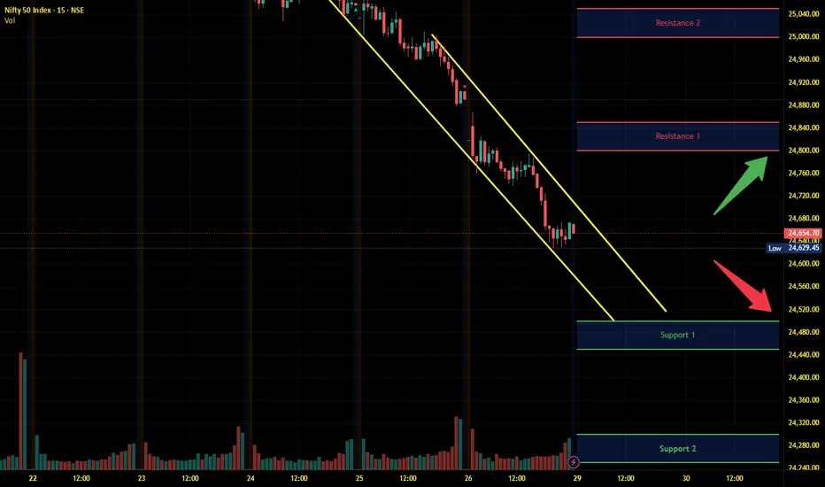
Nifty Intraday Analysis for 29th September 2025NSE:NIFTY
Index has resistance near 24800 – 24850 range and if index crosses and sustains above this level then may reach near 25000 – 25050 range.
Nifty has immediate support near 24500 – 24450 range and if this support is broken then index may tank near 24300 – 24250 range.
Oversold zone, bounce back expected with profit booking on high zone as F&O expiry is nearing.