XAUUSD MULTI TIMEFRAME ANALYSIS Gold looks set to push toward the all-time high without dipping below the previous day’s low. Despite a bearish weekly bias, yesterday’s close makes a deeper move into last week’s low unlikely. Daily structure is bouncing cleanly off the 10/20 EMAs, and the current price action leans strongly bullish. I’ll watch this zone for a high-probability long setup and position toward the upside if my entry conditions trigger.
Harmonic Patterns

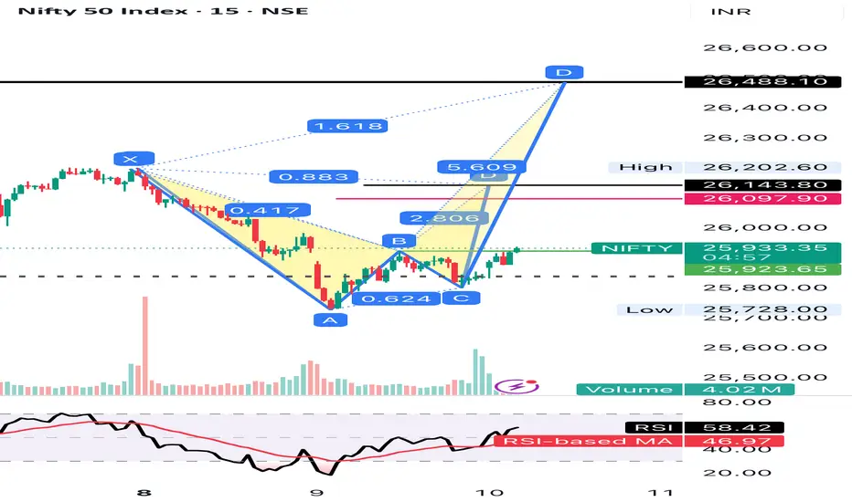
Nifty rally expected soon 26488++ in no timeNifty after hitting 50 EMa ready for rally
Immediate target 26488++
Probably this week only possible
26145/26277 hurdle points
XAUUSD/GOLD JOLTS Job Openings News Projection 09.12.25Main Idea
Gold is currently ranging between 4,191 – 4,210 zones.
During JOLTS news volatility, price may either break upward or break downward from this zone.
Your plan is a breakout + retest entry with a 1:3 Risk–Reward Ratio.
🟢 Bullish Scenario (Buy Setup)
Conditions to Buy:
Price breaks above 4,210 zone
Retests the same zone and holds as support
Enter after bullish confirmation
Target:
4,250 zone
Stoploss:
Below 4,191 zone
🔴 Bearish Scenario (Sell Setup)
Conditions to Sell:
Price breaks below 4,191 zone
Retests the level as resistance
Enter after bearish confirmation
Target:
4,163 zone
Stoploss:
Above 4,210 zone
🎯 Risk–Reward Ratio: 1:3
Both setups aim for a low-risk and high-reward breakout trade using news momentum.

$BNB: Key HTF Decision Zone AheadCRYPTOCAP:BNB : Key HTF Decision Zone Ahead
#BNB is still holding above the critical $700–$550 demand zone, the same area that defines the continuation or breakdown of the current macro trend. As long as price maintains this support, HTF structure stays bullish and the next expansion wave targets $1500 → $2000 → $2500 → $3000.
A weekly close below $550 would flip structure bearish and open a deeper correction toward $250–$170.
Key Levels
Accumulation Zone: $700–$550
Upside Targets: $1500 / $2000 / $2500 / $3000
Invalidation: Weekly close < $550
BNB is at a major decision point: Hold the zone and bullish momentum accelerates; lose it and trend resets.
NFA & DYOR

Divergence Secrets Who Should Trade Options?
Options are suitable for:
Traders looking for leverage with limited risk
Investors wanting to hedge positions
Experienced traders generating income
Anyone willing to learn market structure and volatility
But they require discipline, knowledge, and proper risk management.

GBP/USD – Short Setup Trade Narrative
Price created a lower-high structure after the earlier push up, followed by a sharp sell-off that broke intraday momentum.
A small liquidity grab beneath the prior low caused a corrective pullback into a premium zone, aligning perfectly with the bearish bias.
The current candle shows rejection inside the supply block / retracement zone, giving a clean short entry.
Confluence
Structural lower-high formation
Liquidity sweep before entry
FVG fill during retracement
Higher-timeframe bearish context
Clear risk-to-reward framework

Part 2 Support and ResistanceHow Time Decay Affects Option Traders
Time value decays rapidly near expiry. This is why buyers must be accurate about timing, while sellers benefit from time decay.
Buyers lose money if the market doesn’t move quickly.
Sellers gain even if the market doesn’t move at all.
This is why most experienced traders prefer option selling with risk controls.

Part 1 Support and ResistanceWhat Is Option Premium?
The premium is the price paid by the buyer to the seller to purchase the option. It represents the cost of owning the right.
Premium depends on factors like:
Current market price
Strike price
Time left to expiry
Volatility
Interest rates
Demand and supply
Two components decide the premium:
Intrinsic Value – Real value based on price difference.
Time Value – Extra value because the option has time before expiry.
As expiry approaches, time value decreases — this is called Time Decay (Theta).

Part 12 Trading Master ClassTips for Beginners in Option Trading
1. Start with Buying Options
It reduces your risk while learning market movements.
2. Trade Only One Index First
Start with Nifty or Bank Nifty to understand price behavior.
3. Follow Volume and Open Interest (OI)
These help you understand the market’s real strength.
4. Learn Support & Resistance
Options react strongly at these levels.
5. Avoid Trading During Highly Volatile News
Like RBI policy, Fed meeting, Budget day.
6. Manage Risk
Never put full capital into one trade.
7. Practice Through Paper Trading
Gain confidence before using real money.

Components of a Candle (Body, Wick, High, Low)Types of Candlestick Patterns
Candlestick patterns are broadly divided into:
A. Single Candlestick Patterns
Formed by just one candle.
B. Double Candlestick Patterns
Formed by two-candle combinations.
C. Triple Candlestick Patterns
Formed by three-candle combinations.
Let’s dive into each category in detail.

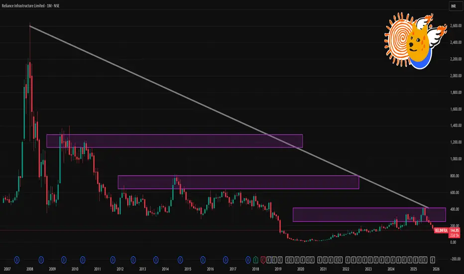
RELINFRA 1 Month Time Frame 📉 What’s Happening Now
As of 8–9 December 2025, Reliance Infrastructure is trading near ₹ 146–147 — its 52‑week low.
Over the past month the stock has seen a sharp drop of ~15–20%.
On 9 Dec it hit a fresh intraday low of ~₹ 139.6‑140, triggering lower‑circuit (i.e. trading halt for the day) — indicating heavy selling pressure.
🔎 Why the Weakness
The recent decline reflects broad selling pressure, partly driven by negative sentiment in its sector and possibly concerns over group‑level regulatory/legal issues.
While the company has been in distress compared with its earlier 52‑week high (~₹ 425), volatility remains high, with the share trading well below major moving averages.
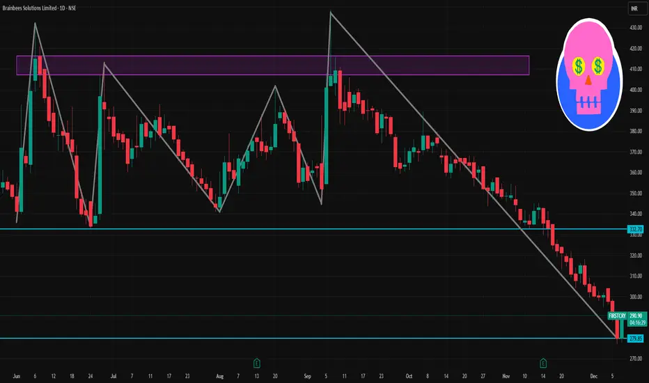
FIRSTCRY 1 Day Time Frame 📊 What the 1‑day chart for Brainbees Solutions currently shows
As of recent trading, the share price of Brainbees Solutions is around ₹ 279–290 on NSE.
The 52‑week high and low band shows a high near ~₹ 664–665 and a low around ~₹ 277–286.
That means at current ~₹ 280–290, the stock is very close to its 52‑week low — which may make the “day‑timeframe level” important for traders looking for a bounce or reversal.
Some technical‑analysis data (on certain days) show bearish momentum: for example, on a recent day the stock hit an all‑time low of ₹ 287, continuing a downtrend.
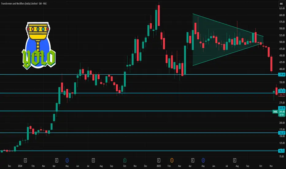
TRIL 1 Week Time Frame 📌 Latest Price & 1‑Week Snapshot
The stock is trading around ₹240–₹241 per share (NSE/BSE).
According to a recent summary, over the last 1 week the stock has moved approximately –7% to –7.4%.
52‑week range: Low ≈ ₹232–₹236, High ≈ ₹648–₹650.
Thus the stock is very near its 52‑week low — down roughly 63% from 52‑week high.
What this suggests (short‑term)
The share is currently at deep discount territory, close to 52‑week bottom — so for traders, this could mean limited downside (barring new negative news), but also that upside is large — albeit requiring major positive triggers.
Given weak near‑term momentum (recent dip, down ‑7% in a week), the stock may consolidate around current levels — ₹230–₹250 zone — unless there’s a strong catalyst.
🎯 What This Means for Short-Term Traders vs Long-Term Investors
Short-term traders: The ₹232–₹240 zone can be considered as a near-term support base. If the stock holds above ~₹235, a bounce is possible — but sharp volatility remains likely. Risk/reward is skewed toward a bounce — but with high uncertainty.
Medium/Long-term investors: The deep discount vs 52‑week high may look attractive — but fundamentals (earnings weakness, recent volatility, sanction overhang) suggest caution. The stock could recover substantially — if the company stabilizes business, wins new orders, and global/sector sentiment improves.
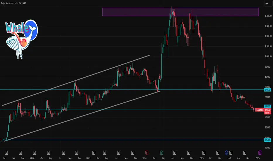
TEJASNET 1 Day Time Frame 📌 Recent Price & Context
According to a live quote on 9 Dec 2025, Tejas Networks is trading around ₹471–₹476.
Recent technical‑indicator feeds (on daily chart) show oversold conditions: e.g. RSI ~ 20 (oversold), MACD negative, ADX high — indicating downward momentum + volatility.
On weekly‑timeframe classification, some aggregator sources rate the trend as “strong sell.”
So at this moment, the bias is bearish to neutral, unless a reversal catalyst emerges.
🎯 Weekly Pivot / Key Levels (Support & Resistance)
Using the most recent weekly pivot analysis:
Level Price (Approx)
Weekly Pivot (central) ₹503.7
Support Zone 1 (S1) ~ ₹482.5
Support Zone 2 (S2) ~ ₹470.9
Resistance 1 (R1) ~ ₹515.3
Resistance 2 (R2) ~ ₹536.5
Resistance 3 (R3) ~ ₹548.0–₹550+
Interpretation
The pivot at ₹503.7 marks the “line of neutrality.” Weekly closes above this level would shift bias more bullish.
As of now, with price ~ ₹472–₹476, the stock is well below weekly pivot → bearish / consolidation regime.
Downside buffer / support lies around ₹470–₹482; a breakdown below that could open further downside risk (unless long‑term support zones hold).
Upside resistance cluster lies at ₹515 → ₹536 → ₹548. To regain bullish momentum, price needs to first clear ₹503–₹515 zone, then aim higher.
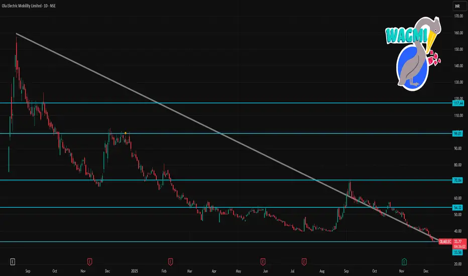
OLAELEC 1 Day Time Frame 📊 Key Daily Levels (Support & Resistance)
From pivot analysis & live technical indicators (today’s data):
Pivot: ~₹34.72
Resistance Levels:
• R1 ~ ₹35.83
• R2 ~ ₹37.56
• R3 ~ ₹38.67
Support Levels:
• S1 ~ ₹32.99
• S2 ~ ₹31.88
• S3 ~ ₹30.15
These are the real-time intraday/daily pivot support & resistance levels traders watch for short term moves.
Alternative pivot data from recent technical sites (slightly different levels):
Pivot: ~₹41.34
Resistance: ~₹41.8 / ₹42.4 / ₹42.9
Support: ~₹40.7 / ₹40.3 / ₹39.7
Options Strategies: Spreads, Straddles, and Iron Condor1. Option Spreads
An option spread involves buying one option and simultaneously selling another option of the same type (call or put) but with different strike prices or expiries. Spreads are primarily used to limit risk, reduce premium cost, or target specific price zones.
Types of Option Spreads
a) Vertical Spreads
A vertical spread uses options with the same expiration date but different strike prices.
There are two kinds:
• Bull Call Spread
Used when the trader is moderately bullish.
Buy a lower-strike call, sell a higher-strike call.
Limits both profit and loss.
Example: Buy 100 CE @ ₹10 → Sell 110 CE @ ₹5 → Net cost ₹5.
• Bear Put Spread
Used when the trader is moderately bearish.
Buy higher-strike put, sell lower-strike put.
Limited profit and limited loss.
Example: Buy 100 PE @ ₹12 → Sell 90 PE @ ₹6 → Net cost ₹6.
• Bear Call Spread
A credit spread for bearish to neutral outlook.
Sell lower-strike call, buy higher-strike call.
Net credit received.
• Bull Put Spread
A credit spread for bullish to neutral outlook.
Sell higher-strike put, buy lower-strike put.
Popular due to high probability of profits.
b) Horizontal (Calendar) Spreads
Calendar spreads use the same strike price but different expiry dates.
When is it used?
When the trader expects low near-term volatility but higher long-term volatility.
It benefits from time decay differences (theta) between near and far expiries.
c) Diagonal Spreads
Diagonal spreads combine both different strikes and different expiries.
Why use them?
To take advantage of both direction and time decay.
More flexible but more complex.
Why Traders Use Spreads
Lower capital requirement.
Defined maximum loss.
Can be structured for any market condition.
Reduce the impact of volatility swings and time decay.
Spreads are ideal for traders who aim for risk-controlled trading instead of outright long or short options.
2. Straddles
A straddle is a highly popular volatility strategy where the trader buys or sells both a call and a put option with the same strike price and same expiry.
a) Long Straddle
Buy 1 Call + Buy 1 Put (ATM).
Used when the trader expects big movement but doesn’t know the direction.
This is a volatility-buying strategy.
Maximum loss = total premium paid.
Profit = unlimited on upside, substantial on downside.
Ideal Conditions
Earnings announcements.
RBI policy decisions.
Major news (mergers, litigation, global events).
Low IV (implied volatility) before expected spike.
Example
NIFTY at 22,000:
Buy 22000 CE @ 120
Buy 22000 PE @ 130
Total cost = ₹250.
If NIFTY moves sharply to either:
22,500 (big CE profit), or
21,500 (big PE profit),
the long straddle gains.
Key Greeks
Vega positive → benefits from IV increase.
Theta negative → loses money from time decay.
b) Short Straddle
Sell 1 Call + Sell 1 Put (ATM).
Used when market is expected to be range-bound with very low volatility.
High risk; unlimited loss potential.
Maximum profit = premiums received.
Why use it?
Only experienced traders use short straddles when:
IV is extremely high.
Market is unlikely to move drastically.
Time decay is expected to be fast.
Short Straddle Risks
Sharp moves can cause heavy losses.
Requires strong risk management and hedge understanding.
3. Iron Condor
An Iron Condor is a neutral, limited-risk, limited-reward option strategy. It combines a Bull Put Spread and a Bear Call Spread.
Structure
Sell OTM Put
Buy further OTM Put
Sell OTM Call
Buy further OTM Call
This creates a structure where the trader profits if the price stays within a range.
Why Traders Love Iron Condors
Designed for markets with low volatility and consolidation.
High probability of winning.
Controlled risk.
Takes advantage of time decay (theta positive).
Payoff Characteristics
Maximum profit occurs when the underlying price stays between the sold call and sold put.
Maximum loss is limited to the width of either spread minus net premium received.
Works best in sideways markets.
Example: NIFTY Iron Condor
Assume NIFTY = 22,000.
Sell 22500 CE
Buy 22700 CE
Sell 21500 PE
Buy 21300 PE
Net credit = Suppose ₹60.
Possible Outcomes
If NIFTY expires between 21,500 and 22,500 → Full profit = ₹60.
If it goes beyond either side → Loss limited to defined spread width.
Ideal Conditions
Market expected to remain in a range.
IV is high before selling, expecting it to fall.
Greeks
Delta neutral
Theta positive (time decay benefits)
Vega negative (falling IV helps)
Comparing the Key Strategies
Strategy Market View Risk Reward Volatility Impact
Vertical Spread Mild bullish/bearish Limited Limited Moderate
Long Straddle High volatility expected Limited Unlimited Needs IV rise
Short Straddle Low volatility expected Unlimited Limited Benefits from IV drop
Iron Condor Sideways / range-bound Limited Limited Benefits from IV drop & theta
How to Choose the Right Strategy
Choosing a strategy depends on:
1. Market Direction
Trending markets → vertical spreads
Unknown direction → straddles
Sideways markets → iron condor
2. Volatility Expectations
IV high? Use credit strategies (short straddle, iron condor).
IV low? Use debit strategies (long straddle, debit spreads).
3. Risk Appetite
Conservative traders: spreads, iron condors.
High-risk traders: short straddles.
Speculators expecting big moves: long straddles.
4. Time Horizon
Short-term: spreads and straddles.
Medium-term: calendar and iron condor.
Conclusion
Spreads, Straddles, and Iron Condors are essential strategies for building an effective options trading system. Each offers unique advantages:
Spreads help control risk and reduce costs.
Straddles capitalize on directional uncertainty and volatility spikes.
Iron Condors profit from sideways markets with predictable risk.
A trader who understands when to apply each strategy based on market behavior, volatility, and risk preference can dramatically improve long-term consistency. Mastering these strategies allows traders to navigate all phases of market conditions—trending, volatile, or stable—using a systematic and well-risk-managed approach.

Sector Rotation & Business Cycles1. Understanding the Business Cycle
The business cycle refers to the natural rise and fall of economic activity over time. It moves through four major phases:
1. Expansion
Economic growth accelerates.
Employment rises, consumer spending increases.
Corporate profits improve.
Interest rates usually remain moderate.
2. Peak
Growth reaches its maximum level.
Inflation may rise.
Central banks often raise interest rates to cool the economy.
Consumer demand becomes saturated.
3. Contraction (Recession)
Economic growth slows.
Corporate earnings weaken.
Layoffs and spending cuts occur.
Stock markets often decline.
4. Trough
Economic decline bottoms out.
Stimulus measures increase (rate cuts, government spending).
Businesses prepare for recovery.
This cyclical movement is driven by consumer behavior, credit cycles, government policy, global factors, and investor sentiment. Although the timing of cycles varies, the behavioral patterns remain largely consistent.
2. Sector Rotation Explained
Sector rotation is the strategy of moving investments from one sector to another based on expectations of the next phase of the business cycle. Investors aim to hold sectors that are likely to benefit from the upcoming environment while avoiding those expected to underperform.
For example:
When interest rates fall and the economy is bottoming out, cyclical sectors often lead.
When inflation rises or recession hits, defensive sectors typically protect the portfolio.
There are three broad groups of sectors to understand:
A. Defensive Sectors
These sectors provide essential goods or services, meaning demand stays stable even during downturns.
Healthcare
Utilities
Consumer Staples
Telecom
These sectors outperform during recessions or slowdowns because people cannot stop spending on necessities like electricity, medicine, and basic household products.
B. Cyclical Sectors
These rise when the economy is strong and fall during recessions.
Consumer Discretionary
Industrials
Financials
Real Estate
Materials
Cyclicals react strongly to consumer confidence and corporate investment.
C. Growth & Inflation-Linked Sectors
These benefit from technological progress or commodity price cycles.
Technology (growth)
Energy (inflation-linked)
Basic Materials (linked to global demand)
3. How Sector Rotation Works Across the Cycle
Here is how major sectors tend to perform during each stage of the business cycle:
1. Early Expansion (Recovery Phase)
Economic Conditions:
Interest rates are low
GDP growth rebounds
Employment picks up
Consumer confidence rises
Winning Sectors:
Consumer Discretionary: People begin buying non-essential goods.
Industrials: Companies increase production and investment.
Financials: Banks benefit from loan growth and improving credit conditions.
Real Estate: Lower interest rates push property demand.
This stage sees some of the strongest equity returns because the market anticipates stronger earnings.
2. Mid Expansion (Strong Growth Phase)
Economic Conditions:
GDP grows steadily
Inflation remains moderate
Corporate profits are strong
Markets remain bullish
Winning Sectors:
Technology: Innovation drives growth.
Industrials & Materials: Increased global demand supports manufacturing.
Energy: Higher consumption raises oil and gas prices.
Tech often dominates in this stage because companies invest in efficiency and automation while consumers adopt new technologies.
3. Late Expansion (Peak Phase)
Economic Conditions:
Growth slows
Inflation increases
Interest rates rise
Market volatility rises
Winning Sectors:
Energy: Inflation boosts commodity prices.
Materials: Benefit from strong but peaking demand.
Utilities (start to gain): Investors seek safety as cycle becomes uncertain.
Investors gradually rotate from growth and cyclical sectors toward safety as interest rates tighten.
4. Contraction (Recession Phase)
Economic Conditions:
GDP declines
Unemployment rises
Corporate profits fall
Credit tightens
Winning Sectors:
Consumer Staples: Essential goods maintain stable demand.
Healthcare: Non-discretionary spending continues.
Utilities: Consumption of power and water remains stable.
Telecom: Communication services are essential.
Defensive sectors outperform because they have predictable cash flows and stable earnings. Meanwhile, cyclical sectors suffer.
5. Trough (Bottoming Phase)
Economic Conditions:
Government and central banks stimulate the economy
Interest rates fall sharply
Economic activity stabilizes
Winning Sectors:
Financials (early recovery)
Consumer Discretionary
Industrials
Technology
Investors anticipate recovery and rotate back into risk assets. This phase often produces high returns for early movers.
4. Factors That Influence Sector Rotation
Sector performance isn’t solely dictated by the business cycle. Other factors influence sector rotation timing and effectiveness:
A. Interest Rates
Higher rates hurt financials, real estate, tech.
Lower rates boost cyclicals and growth stocks.
B. Inflation
High inflation benefits energy, materials, commodities.
Low inflation supports growth sectors like tech.
C. Government Policies
Fiscal spending boosts infrastructure, defense, renewables.
Regulations impact banks, pharma, telecom.
D. Market Sentiment
Fear and greed cycles can accelerate sector rotation—money moves quickly out of risk sectors into defensives during panic.
E. Global Economic Trends
Global demand strongly impacts:
Energy
Materials
Industrials
5. Sector Rotation Strategies for Traders and Investors
Here are the commonly used approaches:
A. Business Cycle Forecasting
Predicting the next phase of the economy and positioning the portfolio ahead of time. Requires macro analysis, economic indicators, and market sentiment tracking.
B. Momentum-Based Rotation
Invest in sectors showing strong price performance and exit those losing momentum. Often used with sector ETFs.
C. Defensive vs. Cyclical Switching
Shift between defensive and cyclical baskets depending on economic signals like:
PMI
Interest rate trends
Inflation data
Yield curve behavior
D. Thematic Sector Rotation
Focus on themes like:
EVs
Artificial Intelligence
Renewable energy
Digital infrastructure
This works well when the economy is neutral but trends drive specific sectors.
6. Benefits of Sector Rotation
Higher Returns: Capture outperforming sectors during each cycle.
Lower Risk: Avoid sectors likely to decline during downturns.
Diversification: Helps spread exposure across industries.
Alignment with Macro Trends: Keeps portfolio positioned for economic shifts.
7. Limitations of Sector Rotation
Timing is challenging.
Economic cycles may be unpredictable.
External shocks can disrupt the pattern (wars, pandemics).
Requires continuous monitoring of macro data.
Conclusion
Sector rotation is one of the most strategic and systematic ways to navigate financial markets. By understanding how sectors behave during different stages of the business cycle and by monitoring key economic indicators, traders and investors can optimize returns, manage risks, and stay ahead of economic changes. Mastering this approach requires discipline, macroeconomic awareness, and adaptability. But when applied correctly, sector rotation becomes a powerful tool for long-term growth and short-term tactical opportunities.
Multi-Timeframe Analysis (MTFA)1. Why Multi-Timeframe Analysis Matters
Markets are fractal in nature—meaning price moves in repeating patterns across all timeframes. A trend visible on the 1-hour chart may simply be a pullback on the daily chart. A breakout on the 5-minute chart may be irrelevant when the weekly trend is sideways.
Relying only on one timeframe creates three common issues:
False breakouts: Lower timeframes give misleading breakouts during higher-timeframe consolidations.
Confusion about trend: The trend on a small timeframe often conflicts with the major trend.
Entries without context: Traders enter without understanding key support/resistance or institutional zones.
MTFA solves all these problems by combining macro and micro views to form decisions rooted in context.
2. The Top-Down Approach (The Standard MTFA Process)
Most traders follow a 3-step method:
Step 1: Identify the Main Trend (Higher Timeframe – HTF)
Use Weekly, Daily, or 4H depending on your style.
Here you look for:
Overall trend direction (uptrend / downtrend / range)
Major support and resistance
Market structure (HH, HL, LH, LL)
Long-term supply and demand zones
HTF gives you the “big picture”—the dominant force of the market.
Step 2: Refine the Setup Zone (Middle Timeframe – MTF)
Use Daily-4H, 4H-1H, or 1H-15M depending on the trade.
This timeframe helps confirm:
Trend alignment
Pullbacks
Break of structure
Chart patterns (flags, triangles, channels)
Key levels where entries may occur
MTF filters out low-probability setups and identifies accurate zones.
Step 3: Execute With Precision (Lower Timeframe – LTF)
Use 1H, 15M, 5M, or 1M for exact entries.
This timeframe helps you:
Time entries
Catch liquidity grabs
Place tight stop-losses
Monitor candle patterns (pin bars, engulfing, doji)
Confirm momentum using volume/RSI/stochastic
This is where the actual trade triggers happen.
3. Choosing the Right Timeframes (Based on Trading Style)
Different trading styles require different combinations.
1. Scalpers
HTF: 1H
MTF: 15M
LTF: 1M–5M
Goal: Quick moves, tight SL, small targets.
2. Intraday Traders
HTF: Daily
MTF: 1H
LTF: 5M–15M
Goal: Catch day moves with strong accuracy.
3. Swing Traders
HTF: Weekly
MTF: Daily
LTF: 4H
Goal: Hold trades for days to weeks.
4. Position Traders
HTF: Monthly
MTF: Weekly
LTF: Daily
Goal: Capture major multi-month trends.
The key rule:
The larger timeframe decides trend direction; the smaller timeframe decides entry timing.
4. How MTFA Improves Trading Accuracy
1. Identifying True Trend Direction
A rise on the 15-minute chart may look bullish, but on the daily chart it may be a simple retracement in a strong downtrend. MTFA prevents trading against the dominant direction.
2. Avoiding Market Noise
Lower timeframes contain lots of fake moves (whipsaws). MTFA filters them out by relying on higher-timeframe structure.
3. Improved Entry and Exit
You can wait for precise structure breaks or candle confirmations on smaller timeframes while holding the higher-timeframe bias.
4. Better Risk Management
Since entries become more accurate, stop-loss distance reduces while keeping the same reward potential, thus improving risk-to-reward ratio (RRR).
5. Practical MTFA Example (Bullish Scenario)
Let’s say you are analyzing a stock or index.
Weekly Chart
Showing a clear uptrend (higher highs and higher lows).
Price currently retracing toward a major support zone.
Bias: Long (buy).
Daily Chart
Shows a bullish reversal pattern—like a double bottom or bullish engulfing candle.
Market structure shifts from lower lows to higher lows.
Bias strengthened: Prepare for long entries.
1-Hour Chart
Shows break of a short-term downward trendline.
A pullback retests a demand zone.
Entry triggers form: pin bar, engulfing, volume spike.
Execution: Enter long with confidence.
Here:
HTF gave direction.
MTF confirmed reversal.
LTF gave precision timing.
6. Understanding Conflicts Between Timeframes
Sometimes timeframes disagree:
Daily is bullish, but 1H is bearish.
4H shows consolidation, but 15M shows breakouts.
This is normal.
Rule:
The higher timeframe always overrides the lower timeframe.
If the HTF is bullish and LTF is bearish, the bearish move is likely a retracement—not a reversal.
Only when HTF breaks its structure should you consider changing bias.
7. Tools and Indicators Used in MTFA
MTFA does not depend on indicators, but indicators can support analysis.
Useful Tools
Price Action & Candlestick Patterns
Market Structure (HH, HL, LH, LL)
Support & Resistance Levels
Trendlines & Channels
Supply and Demand Zones
Helpful Indicators
Moving Averages (20/50/200) – for trend confirmation
RSI or Stochastic – for momentum and overbought/oversold
Volume – confirms strength of breakouts
MACD – for trend shifts
Key rule:
Indicators can support, but higher timeframe structure must lead the analysis.
8. Common MTFA Mistakes to Avoid
1. Overusing Too Many Timeframes
Using more than 3–4 creates confusion.
Stick to a simple framework: HTF + MTF + LTF.
2. Taking Trades Against the Higher-Timeframe Trend
This results in low-probability trades.
3. Forcing Breakouts on Small Timeframes
A breakout on 5M may be meaningless if the daily timeframe is in a strong range.
4. Not Waiting for Alignment
All timeframes must agree before entering.
5. Ignoring Key Levels
Higher-timeframe S/R zones are where major institutions trade.
9. Benefits of Mastering MTFA
Increases trade accuracy
Reduces emotional trades
Provides clear market structure
Helps catch major moves
Improves reward-to-risk
Builds professional-level discipline
Works in any market (stocks, forex, crypto, commodities, indices)
10. Summary of Multi-Timeframe Analysis
MTFA combines higher, middle, and lower timeframe views.
Higher timeframe shows trend and major levels.
Lower timeframe shows entry and precision.
MTFA avoids noise, false breakouts, and misleading signals.
It enhances risk management and trade quality.
All successful traders use MTFA, from scalpers to swing traders.
Market Participants: Retail, FII, DII, HNI & Market Makers1. Retail Investors
Retail investors are individual, non-professional participants who invest their personal capital in stocks, mutual funds, derivatives, or other financial instruments. They are the largest group in terms of numbers but typically hold small portions of total market capitalization.
Key Characteristics
Invest smaller amounts compared to institutions
Use brokers, mobile apps, and trading platforms
Often influenced by news, trends, macro events, and market sentiment
Tend to have shorter time horizons, especially in intraday and swing trading
Behaviour sometimes driven by emotions like fear and greed
Role in the Market
Retail participation adds diversification and liquidity, especially in mid-cap and small-cap stocks. During bull markets, retail traders often amplify momentum, while in bear markets, panic selling from retail segments may accelerate declines.
Strengths
Agile and quick to enter or exit
Access to vast free learning materials and trading tools
Ability to participate in IPOs, ETFs, and systematic investment plans (SIPs)
Weaknesses
Limited capital
High risk of emotional decision-making
Often lack deep research or institutional-grade analytics
Despite limitations, retail participation has dramatically increased due to digital broking, lower costs, and financial awareness.
2. Foreign Institutional Investors (FIIs)
Foreign Institutional Investors include global funds, hedge funds, pension funds, sovereign wealth funds, and international asset managers who invest in Indian markets. They trade large volumes and are among the most influential market movers.
Key Characteristics
Very large capital base
Data-driven, research-driven, algorithmic, and sophisticated
Focus on long-term macro trends—GDP growth, interest rates, inflation, and currency movement
Their inflows/outflows cause significant swings in index levels
Impact on Markets
FIIs play a dominant role in Indian equity and debt markets. When FIIs buy heavily, markets usually rise due to high liquidity infusion. When they sell, markets often see corrections.
What Influences FIIs?
Global interest rates (especially US Fed)
Geopolitical stability
Exchange rate (INR vs USD)
Corporate earnings in emerging markets
Global risk appetite (risk-on vs risk-off sentiment)
Strengths
Access to advanced models, research, and analytics
Ability to influence sectors like banking, IT, and large-cap indices
Long-term disciplined investing strategies
Risks
FIIs can pull money suddenly, causing sharp volatility
Their decisions often depend on global—not domestic—factors
Heavy dependence on currency fluctuations
FIIs bring credibility and stability but also volatility when exiting in large quantities.
3. Domestic Institutional Investors (DIIs)
Domestic Institutional Investors include Indian mutual funds, insurance companies, banks, pension funds, and other local financial institutions. DIIs have grown rapidly in the last decade due to rising SIPs and increased financial literacy.
Key Characteristics
Large domestic capital base
Often counterbalance FII moves
Long-term view aligned with Indian economic growth
Invest systematically through mutual fund inflows
Examples include LIC, SBI Mutual Fund, HDFC Mutual Fund, ICICI Prudential, UTI, etc.
Role in Market Stability
DIIs play a stabilizing role, especially when FIIs sell aggressively. Their consistent inflows help maintain market confidence. For example, during global uncertainty periods, DIIs often cushion sharp falls.
Strengths
Strong understanding of domestic economic conditions
Long-term approach reduces volatility
Backed by consistent retail SIP inflows
Weaknesses
May follow conservative strategies
Sometimes influenced by government or regulatory constraints
Less aggressive compared to FIIs in certain sectors
Overall, DIIs are becoming increasingly powerful and are expected to dominate long-term market behavior in India.
4. High-Net-Worth Individuals (HNIs)
HNIs are individuals with substantial personal wealth (typically ₹5 crore+ net worth). They actively participate in equity, derivatives, PMS (Portfolio Management Services), AIFs (Alternative Investment Funds), and IPOs.
Key Characteristics
Invest large personal capital
Often use professional advisors or portfolio managers
Strong presence in pre-IPO placements, SME IPOs, and block deals
Engage in high-risk strategies like derivatives, arbitrage, and leveraged trades
Market Influence
Though smaller than FIIs/DIIs in size, HNIs influence short-term trends, especially in:
IPO subscriptions (NII category)
Penny stocks and small caps
High-volume derivative positions
Strengths
Flexibility like retail, power like institutions
Can take concentrated bets
Access to exclusive opportunities (AIFs, PMS, private equity)
Weaknesses
Risk of overexposure due to large positions
Sensitive to market cycles
May follow speculative strategies
HNIs bridge the gap between retail traders and large institutions.
5. Market Makers
Market makers are financial institutions or professionals who provide continuous buy and sell quotes in the market to ensure liquidity. They are essential for smooth trading, especially in derivatives, ETFs, currency markets, and less-liquid stocks.
Key Characteristics
Quote both Bid (buy) and Ask (sell) prices
Profit from the bid-ask spread
Use algorithmic and high-frequency trading systems
Licensed or registered under exchange rules
Examples include global firms like Virtu Financial, Citadel Securities, and domestic brokerage proprietary desks.
Role in the Market
Ensure liquidity by always being ready to trade
Reduce volatility by narrowing price gaps
Help large trades get executed smoothly
Vital for ETFs—without them, ETF prices may not track underlying assets
Strengths
High-speed execution
Deep risk management systems
Help maintain orderly markets
Risks
Exposed to sudden volatility during black-swan events
Algorithm failures can cause temporary mispricing
Spread-based profits reduce in highly efficient markets
Without market makers, many securities would suffer from low liquidity and high transaction costs.
How These Participants Interact
Markets behave like a battlefield of different capital sizes and intentions:
FIIs drive major trends with large inflows/outflows.
DIIs stabilize markets with consistent buying during volatility.
HNIs move selectively, especially in IPOs and derivatives.
Retail investors amplify momentum in trending markets.
Market makers maintain liquidity, enabling smooth execution.
Their combined actions create price discovery, the fundamental mechanism determining stock prices.
Final Thoughts
Understanding market participants helps traders decode price movements more logically. Retail traders often observe FII–DII data, volume patterns, and liquidity behavior to align their trades. FIIs and DIIs shape long-term trends, HNIs influence medium-term sentiment, and market makers ensure constant liquidity.
As markets mature, the interaction among these participants becomes more dynamic, making it essential for investors to study their behavior to improve decision-making, timing, and risk management.

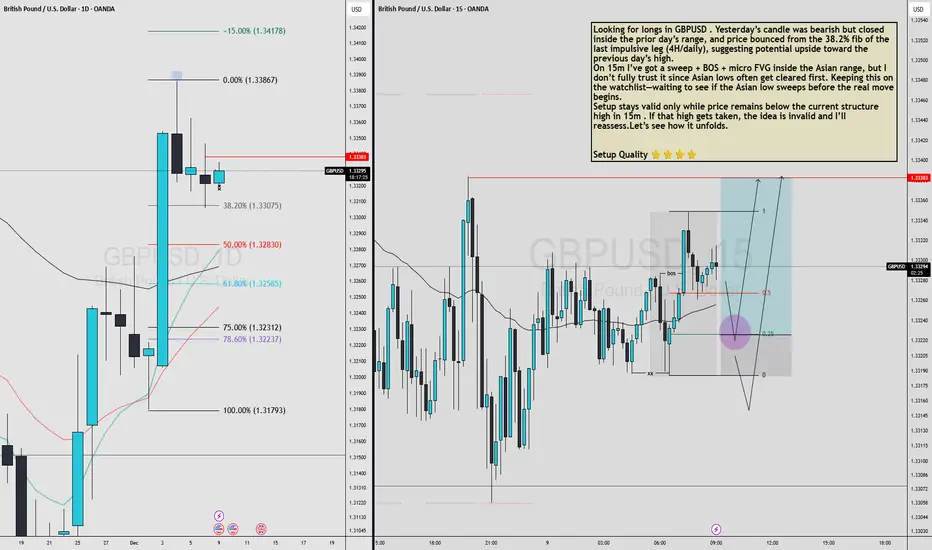
GBPUSD MULTI TIMEFRAME ANALYSIS Looking for longs in GBPUSD . Yesterday’s candle was bearish but closed inside the prior day’s range, and price bounced from the 38.2% fib of the last impulsive leg (4H/daily), suggesting potential upside toward the previous day’s high.
On 15m I’ve got a sweep + BOS + micro FVG inside the Asian range, but I don’t fully trust it since Asian lows often get cleared first. Keeping this on the watchlist—waiting to see if the Asian low sweeps before the real move begins.
Setup stays valid only while price remains below the current structure high in 15m . If that high gets taken, the idea is invalid and I’ll reassess.Let’s see how it unfolds.
Setup Quality ⭐⭐⭐⭐
NIFTY- Intraday Levels - 9th December 2025Only few bullish levels (without buffer) are marked on chart 26033/56 seems to be make or break level.
If NIFTY sustain below 25938 below this bearish then 25892/74 support below this more bearish then 25843/30 strong level this is the same price were market made open= low on 26th nov very very strong level and last hope 25761 below this wait
My view :-
"My viewpoint, offered purely for analytical consideration, The trading thesis is: Nifty (bullish tactical approach: buy on dip) The market is anticipated to form a floor (bottom).
This analysis is highly speculative and is not guaranteed to be accurate; therefore, the implementation of stringent risk controls is non-negotiable for mitigating trade risk."
Consider some buffer points in above levels.
Please do your due diligence before trading or investment.
**Disclaimer -
I am not a SEBI registered analyst or advisor. I does not represent or endorse the accuracy or reliability of any information, conversation, or content. Stock trading is inherently risky and the users agree to assume complete and full responsibility for the outcomes of all trading decisions that they make, including but not limited to loss of capital. None of these communications should be construed as an offer to buy or sell securities, nor advice to do so. The users understands and acknowledges that there is a very high risk involved in trading securities. By using this information, the user agrees that use of this information is entirely at their own risk.
Thank you.

RENDER will hit $15?CRYPTOCAP:RENDER Technical Update
Price is in a bearish corrective phase and currently reacting at the 0.618 Fib zone ($1.55–$1.25), A key area for potential bullish reversal. Holding this zone increases the probability of a strong upside continuation toward $4.6 / $8 / $13 / $20.
If this support breaks, the next major demand lies at the 0.786 Fib level (~$0.84), considered the optimal accumulation zone before any trend shift.
Key Zones:
0.618 Support: $1.55–$1.25
0.786 Support: $0.84
Targets: $4.6 / $8 / $13 / $20
NFA Always DYOR

USDJPY MULTI TIMEFRAME ANALYSIS USDJPY’s long-term and daily trend remain bullish, and today’s candle is closing strong above the 10 EMA—clear momentum resuming after the corrective pullback. On 15m I’ve got a clean sweep + BOS + FVG. I’m waiting for a pullback into my level during Asia/Frankfurt/London. First target: previous day’s high; second: 156.180.
If the previous day’s high clears before my entry triggers, the setup becomes invalid and I’ll reassess. The entry also lines up with a 4H flip zone where former resistance may act as support. Let’s see how it unfolds.
Setup quality ⭐⭐⭐⭐⭐
