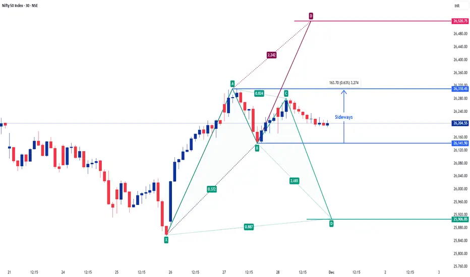
#Nifty Weekly 01-12-25 to 05-12-25#Nifty Weekly 01-12-25 to 05-12-25
26100-26300 is the sideways range(no trade zone for option buyers) for next week.
If Nifty sustains above 26320, ABCD gets activated and targets are 26400/26500.
If Nifty trades below 26100. XABCD gets activated and targets are 26000/25900.
View: Sideways to bearish, reason is Divergence in Higher TF's.
Harmonic Patterns
Markets are RIGGED?Most traders begin their journey believing that the market will test their strategies, their indicators, and their ability to forecast price movements.
But the truth is far more uncomfortable:
The market tests you.
Your beliefs.
Your fears.
Your discipline.
Your identity.
You don’t trade the markets —
you trade your psychology.
The chart is merely the mirror.
Every hesitation, every impulse entry, every oversized position, every revenge trade…
These are not market behaviors.
They are your behaviors showing up on the screen.
You get exposed as a person the moment you start trading.
Not publicly — but inwardly.
You see the parts of yourself you could ignore in normal life:
• Your impatience
• Your fear of missing out
• Your need to be right
• Your avoidance of uncertainty
• Your emotional triggers
• Your lack of preparation
• Your fantasies and biases
The market makes them visible. It forces you to confront them.
And that’s why mastering yourself is the real edge.
Not a new indicator.
Not a new setup.
Not a new piece of news flow.
The internal work — discipline, emotional clarity, self-control, and self-awareness — creates the conditions for consistent execution. Without this inner alignment, even the best strategy collapses under emotional pressure.
When you hold your breath during a trade, the chart isn’t the problem.
When you hesitate to press the buy button, the trend isn’t the problem.
When you panic-exit a position early, volatility isn’t the problem.
Your inner state is what shapes your trading decisions.
That’s why your outside life is inseparable from your trading life.
How you:
• manage stress
• respond to conflict
• handle uncertainty
• maintain discipline
• structure your daily routine
• treat yourself during setbacks
• set boundaries
— all of this shows up in your trading results.
If your life lacks structure, your trades will lack structure.
If you avoid discomfort, you’ll avoid executing good trades.
If you’re emotionally reactive outside the markets, you’ll be reactive inside them.
If you’re scattered mentally, your entries will be scattered too.
Your personal patterns become your trading patterns.
Trading doesn’t change you — it reveals you.
And that’s why traders who commit to self-mastery eventually rise above the noise.
They aren’t fighting the market anymore.
They’ve learned to stop fighting themselves.
The graphs become quieter.
The impulses weaken.
The noise fades.
Decisions become clearer, calmer, cleaner.
Because the trader has changed —
and the trading reflects that change.

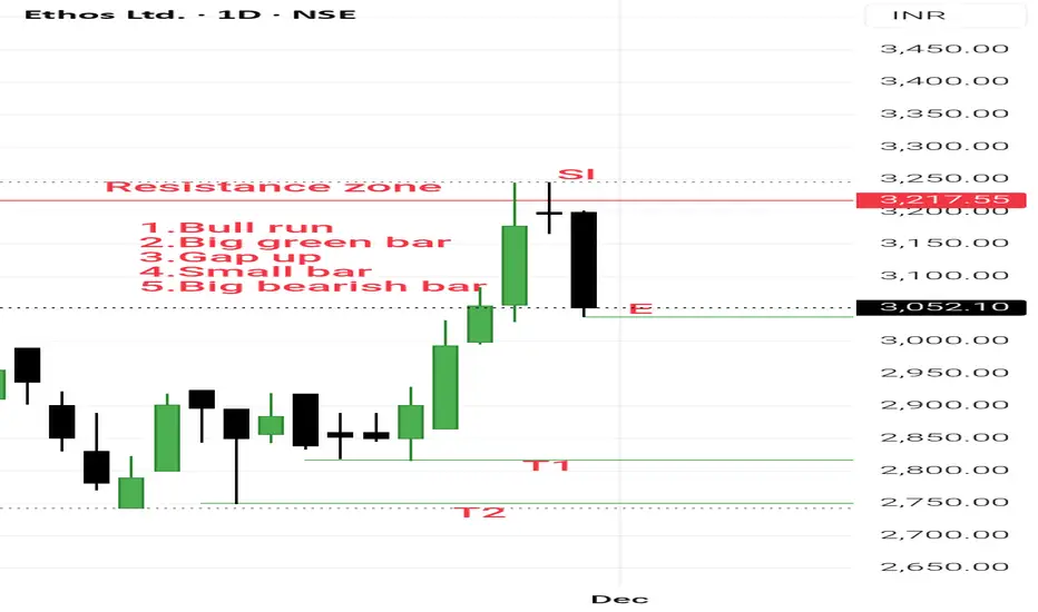
ETHOS ETHOS forming evening star pattern near resistance zone on daily time frame.
No buy/sell recommendation. Only for education purpose.
Alembic Pharma — After 100-Day ConsolidationAlembic Pharma has spent nearly 100 days in a tight consolidation box, holding above major support while maintaining a higher-high, higher-low structure on the long-term (1400-day) chart. This combination strongly favors a bullish continuation breakout.
Technical Outlook (Bullish Bias)
Price has remained inside a narrow consolidation band for ~100 days. Such extended compression typically leads to a single-direction strong move.
Strong Support: ~₹900 zone
Primary Resistance / Breakout Zone: ~₹968
Primary Target Post-Breakout: ~₹1,111
Short-Term Extended Target: ~₹1,289
Breakdown Risk Level: ~₹723 (only if support fails)
Fundamental Drivers Supporting the Bullish View
Latest consolidated Revenue (Q2 FY26) ₹ 1,910.15 crore — ↑ +16% YoY
Latest consolidated Profit After Tax (PAT) Q2 FY26 ₹ 185 crore — ↑ ≈ +21% YoY
EBITDA Margin (recent quarter) ~ 17%
R&D Investment (Recent) ~ 10% of revenue — investing in complex generics & injectables The 16% topline growth and 21% PAT growth in the latest quarter indicate improving operational performance and margin recovery.
Strong EBITDA margin (~17%) and healthy profits suggest the company is handling competition and cost pressures well — a positive sign.
Regular USFDA approvals and robust R&D commitment point to future product launches, which can boost export revenues and long-term growth potential.
52-Week Price Range Low: ₹ 725.20 / High: ₹ 1,123.95
Directional Trading Plan (Bullish)
Breakout Entry
• Buy on daily close above ₹968
• Confirm breakout with above-average volume
Targets
• Primary Target: ₹1,111
• Extended / Short-Term Target: ₹1,289
Stop-Loss
• SL below ₹900 (strong support and consolidation floor) Break below this invalidates the bullish thesis.
Aggressive Alternative Entry
• Buy near ₹900–₹910 on dips (only if price shows reversal candle + support holds)
Disclaimer: aliceblueonline.com

ETH Could Skyrocket to $7.8K After FUSAKA Upgrade: History ShowsCRYPTOCAP:ETH Could Skyrocket to $7.8K After FUSAKA Upgrade – History Shows
The last Ethereum Pectra Upgrade on 7 May 2025 triggered a massive move:
✅ +55% in 35 days
✅ +168% in 109 days
What’s next?
The FUSAKA Upgrade is scheduled for 3 December 2025. If history repeats:
👉 Target 35 days post-upgrade: $4,500 (7 Jan 2026)
👉 Target 109 days post-upgrade: $7,800 (22 Mar 2026)
Note: This is Purely Fractal Analysis Based on Pectra. Always DYOR – Markets can behave differently, and “Sell the News” Scenarios Happen.
Get ready for a potential ETHEREUM rally!
NFA & DYOR

Part 7 Trading Master Class Why Traders Use Options
1. Hedging
Investors use options to protect their portfolios from downside risk.
Example: Buying a put option acts like insurance.
2. Speculation
Options allow traders to take directional bets with limited capital.
3. Income Generation
Selling options (covered calls, cash-secured puts) generates regular income through premium collection.
4. Leverage
Options enable traders to control large positions with small capital.

Market Rotations in the Indian Stock MarketIntroduction
Market rotation is a concept widely used by investors and traders to understand how different sectors perform at various stages of the economic cycle. It refers to the movement of capital from one sector or asset class to another, often driven by economic trends, interest rate changes, government policies, or global market dynamics. In the Indian context, understanding market rotations is crucial due to the market's sectoral diversity and the influence of both domestic and international factors.
The Indian stock market, represented mainly by indices like the Nifty 50 and BSE Sensex, consists of multiple sectors such as Banking, IT, Pharmaceuticals, FMCG, Energy, Metals, and Infrastructure. Each sector reacts differently to economic conditions, and rotations across these sectors present opportunities for investors to optimize returns and reduce risks.
1. Understanding Market Rotation
Market rotation is essentially about capital flow between sectors. Investors rotate funds based on valuation, growth potential, interest rates, and macroeconomic trends. For example, during economic expansion, cyclical sectors like Banking, Automobiles, and Capital Goods tend to outperform, while defensive sectors like FMCG and Pharmaceuticals are preferred during economic slowdowns.
In India, rotations are influenced by:
Domestic factors: GDP growth, inflation, RBI policy rates, fiscal policies, and political developments.
Global factors: Crude oil prices, global interest rates, foreign institutional investor (FII) flows, and geopolitical risks.
2. Types of Market Rotations
Sector Rotation:
Movement of funds between sectors based on macroeconomic trends. Example: Investors move from IT and Pharma (defensive) to Banking and Auto (cyclical) during economic expansion.
Style Rotation:
Rotation between investment styles such as growth stocks and value stocks, or between large-cap, mid-cap, and small-cap stocks.
Asset Class Rotation:
Movement between different asset classes, e.g., equities to bonds or gold, often triggered by interest rate changes or global uncertainty.
3. Importance of Market Rotations
Understanding market rotations is crucial for multiple reasons:
Maximizing Returns: By following rotation trends, investors can position themselves in sectors likely to outperform.
Risk Management: Rotation helps avoid overexposure to underperforming sectors.
Timing Investments: Helps investors decide when to exit a sector that has peaked and enter one with higher potential.
Portfolio Diversification: Enhances risk-adjusted returns by shifting between cyclical and defensive sectors according to market phases.
4. Economic Cycles and Sector Performance in India
Market rotations often mirror the economic cycle, which can be broadly divided into four phases:
Early Expansion:
Characterized by recovery from recession, rising industrial production, and corporate earnings growth.
Sectors to watch: Capital Goods, Metals, Infrastructure, Auto.
Example: Post-pandemic India (2021-22) saw significant rotation into capital-intensive sectors due to economic revival and government infrastructure push.
Late Expansion:
Economic growth continues, but inflationary pressures increase.
Sectors to watch: Banking, Finance, Consumer Discretionary.
Example: During periods of strong credit growth, NBFCs and private banks often outperform.
Early Contraction / Slowdown:
Economic growth slows; earnings decline; interest rates may rise to control inflation.
Sectors to watch: FMCG, Pharmaceuticals, Utilities.
Reason: Defensive sectors maintain stable cash flows even during slowdown.
Recession:
Economic contraction, high unemployment, low consumption.
Sectors to watch: Gold, FMCG, Pharma.
Reason: Investors move to safe-haven assets and defensive equities.
5. Key Indian Sectors and Their Rotation Patterns
Banking & Financials:
Highly sensitive to interest rate cycles and credit growth.
Outperform during economic expansion and low interest rates.
Rotation cue: RBI policy changes, credit demand, and NPA trends.
IT & Software Services:
Considered defensive due to global revenue streams and recurring contracts.
Perform steadily during slowdowns but may lag during domestic growth surges.
Pharmaceuticals & Healthcare:
Defensive sector; stable revenue even during recessions.
Gains rotation interest during global uncertainty or domestic slowdown.
FMCG & Consumer Staples:
Defensive; high demand regardless of economic cycles.
Attract capital during slowdown and high inflation periods.
Automobile & Capital Goods:
Cyclical; benefit from rising disposable income and industrial demand.
Rotation flows in during early and late expansions.
Energy & Metals:
Sensitive to commodity prices and global demand.
Rotate in when industrial growth accelerates and global commodity prices rise.
6. Drivers of Market Rotation in India
RBI Monetary Policy:
Interest rate hikes often lead to rotation into defensive sectors like FMCG and Pharma.
Rate cuts encourage capital flow into cyclical sectors like Banking and Auto.
Government Policies:
Infrastructure spending or PLI schemes can trigger rotation into Capital Goods, Metals, and Electronics sectors.
Global Events:
Oil price spikes, US Fed rate decisions, and geopolitical risks influence rotations between Energy, IT, and Gold.
Valuation & Earnings:
Overvalued sectors see outflows, while undervalued sectors attract capital.
Investors rotate based on relative performance and P/E ratios.
Foreign Institutional Investor (FII) Flows:
FIIs significantly impact Indian markets. Strong inflows can rotate sectors like Banking, IT, and Pharma, while outflows often trigger a move to safe-haven sectors.
7. Strategies for Investors
Identify Macro Trends:
Track GDP growth, inflation, interest rates, and government policies to anticipate sectoral performance.
Follow Institutional Activity:
Monitor FII and domestic institutional investor (DII) flows to spot potential rotations.
Technical & Fundamental Analysis:
Use charts and valuation metrics to identify sectors or stocks ready for rotation.
Diversification Across Sectors:
Maintain exposure to both cyclical and defensive sectors to reduce risk.
Timing and Discipline:
Avoid chasing momentum; enter sectors early in rotation trends and exit before they peak.
8. Practical Examples of Market Rotation in India
2014-2015: Expansion in infrastructure and capital goods due to government’s Make in India initiative; rotation from defensive sectors to cyclical sectors.
2020-2021: Post-COVID economic recovery saw rotation into IT, Pharma, and FMCG sectors initially, followed by Banking and Auto as domestic demand revived.
2022-2023: Rising interest rates triggered rotation from rate-sensitive Banking to defensive FMCG and Pharma sectors.
9. Challenges in Predicting Rotations
Market Sentiment: Emotional trading can distort rational rotations.
Global Correlations: International shocks (oil, interest rates, geopolitical risks) can abruptly change rotation patterns.
Lag in Economic Data: Market reacts faster than published economic indicators.
Sector Concentration Risks: Over-reliance on one sector can magnify losses if rotation timing is wrong.
10. Conclusion
Market rotation is a powerful concept for Indian investors and traders seeking to maximize returns while managing risk. By understanding economic cycles, sector-specific drivers, and investor behavior, one can anticipate where capital is likely to flow next. In India’s diverse and dynamic market, rotation between defensive and cyclical sectors, as well as across asset classes, provides ample opportunities for disciplined and informed investors.
Successful rotation strategies require macroeconomic awareness, monitoring of institutional flows, valuation analysis, and timing discipline. While no strategy is foolproof, integrating market rotation principles into investment decisions can significantly enhance portfolio performance over time.

Vimta Labs Limited - Breakout Setup, Move is ON...#VIMTALABS trading above Resistance of 607
Next Resistance is at 1113
Support is at 498
Here are previous charts:
Chart is self explanatory. Levels of breakout, possible up-moves (where stock may find resistances) and support (close below which, setup will be invalidated) are clearly defined.
Disclaimer: This is for demonstration and educational purpose only. This is not buying or selling recommendations. I am not SEBI registered. Please consult your financial advisor before taking any trade.

Vimta Labs Limited - Breakout Setup, Move is ON...#VIMTALABS trading above Resistance of 952
Next Resistance is at 1214
Support is at 691
Here are previous charts:
Chart is self explanatory. Levels of breakout, possible up-moves (where stock may find resistances) and support (close below which, setup will be invalidated) are clearly defined.
Disclaimer: This is for demonstration and educational purpose only. This is not buying or selling recommendations. I am not SEBI registered. Please consult your financial advisor before taking any trade.

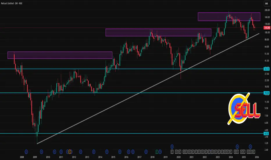
NELCAST 1 Month Time Frame 📌 Recent snapshot
As of 28 Nov 2025, Nelcast closed around ₹116.
Over the past 1 month, the stock has seen a ~ –9 % return.
The 52-week trading range: low ~ ₹78, high ~ ₹180.
✅ My View (with caution)
Nelcast seems fairly valued — perhaps a bit stretched relative to estimated intrinsic value. In short term (1 month), a range between ₹112–₹125 seems the most probable, unless there’s a sharp catalyst (good or bad).
If I were you — and purely for trading or short-term view — I’d watch for a dip toward ₹110–₹112 (as a possible “buy zone / entry”) and a rebound toward ₹124–₹125.
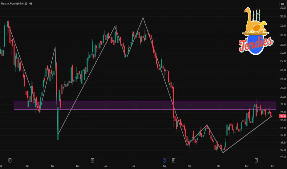
MARKSANS 1 Day time Frame 📌 Current Price & Broad Context
Latest share price: ≈ ₹187.95.
52-week range: Low ~ ₹162.00, High ~ ₹358.70.
Recent trend: The stock is significantly below its 52-week high; price has fallen roughly 25–45% over the past 6–12 months.
🧮 What to Watch / Combine with Other Views
Daily technicals show neutral-to-bearish bias, with some structural support around long-term moving average.
But longer-term fundamentals (company financials, order book, approvals, sector sentiment) could disrupt this — technicals are just one lens.
Because the stock is well below its 52-week high, there’s scope for rebound — but also risk: price could continue downward if sentiment remains weak.
For better clarity: it’s often helpful to check 1-week or 1-month charts along with volume, open interest (if derivatives), and any corporate/news events.
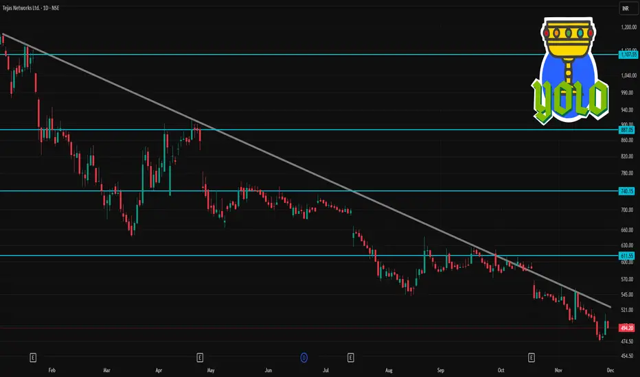
TEJASNET 1 Day Time Frame 📌 Current Price & Context
Recent data shows TEJASNET trading around ₹494–₹496.
52-week range: Low ~ ₹474.45, High ~ ₹1,402.70.
On 1-day/short-term technicals: the consensus remains “Sell / Strong Sell”.
So — the stock is near its lower end of the 52-week range, but short-term momentum is weak.
✅ What This Means for Traders (1-Day / Intraday)
As of now, bias on 1-day timeframe remains bearish / neutral. Unless there is a strong positive catalyst, further downside or consolidation is more likely than a sustained bounce.
The zone around ₹484–₹486 (and possibly down to ₹471–₹475) is critical support — a breakdown below could open a bigger downside swing.
On the upside, watch ₹511–₹512 and then ₹520–₹525 for any meaningful resistance breaks — only a close above these may suggest short-term relief.
Because moving averages are well above current price, any upside rally may remain limited unless volume and market-wide sentiment improve.
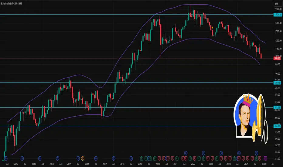
BATAINDIA 1 Month Time Frame 📌 Recent Price & Context
The stock has recently traded around ₹1,000–₹1,010 levels.
The 52-week high is ~₹1,479; 52-week low is ~₹996–₹1,005 (depending on the source) — so recent levels are close to the lower end of the 52-week range.
The stock has been under pressure lately, partly due to weak Q2 FY26 results which dragged sentiment.
⚠️ Key Risks & What’s Dragging the Stock
Weak recent financial performance — recent quarter’s poor results have weighed on sentiment.
Technical picture remains weak: price below all major moving averages, multiple sell signals on daily charts.
High volatility and lack of clarity on demand — any bounce may be shallow unless firm positive triggers come (e.g. good sales data, broader market up-move, sector tailwinds).
Part 4 Learn Institutional TradingParties Involved in an Options Contract
There are two sides to every options contract:
Option Buyer
Pays the premium.
Has limited risk (only the premium paid).
Has unlimited profit potential in call options and significant potential in puts.
Option Seller (Writer)
Receives the premium.
Has limited profit (only the premium collected).
Faces potentially unlimited risk in calls and large risk in puts.
Option sellers generally need higher margin because they take the greater risk.

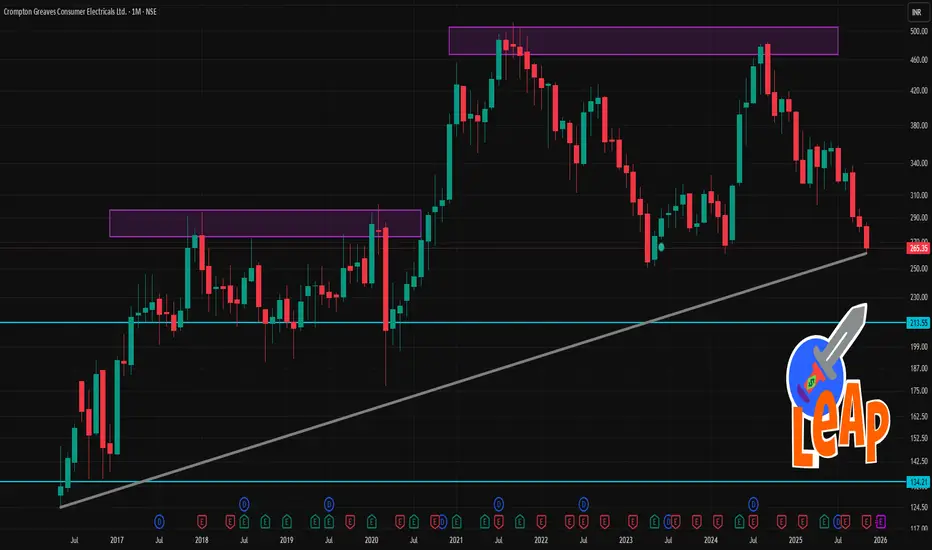
Crompton 1 Month Time Frame 📉 Recent context & background
The stock recently hit a fresh 52-week low — around ₹267.5–₹271.25.
Latest quarter (Q2 Sep-2025) saw a sharp profit drop: net profit fell ~43% YoY, with EBITDA margin under pressure due to commodity cost inflation and restructuring costs.
On the flip side, the company’s broader business mix (like pumps / small domestic appliances / solar-rooftop orders) and some analyst estimates still see potential for recovery.
🧭 What could move the price in next 1 month
Positive triggers: Any signs of margin recovery, easing of commodity inflation, good order wins (e.g. solar-segment orders or domestic appliance demand), supportive news or institutional interest.
Negative triggers: Continuation of margin pressure, weak demand in core categories, negative macro / interest-rate or inflation environment, or broader investor risk-off sentiment.
🎯 My Base-Case 1-Month Scenarios
Bearish to neutral scenario: Price may hover or drift around ₹260–₹285, possibly bouncing between support (₹265–₹270) and resistance (₹280–₹290).
Bullish/recovery scenario: If sentiment improves, stock could aim for ₹300–₹330 over the next 3–4 weeks — especially if company provides encouraging updates or sector environment improves.
Upside breakout scenario (less likely in short 1-month): A push toward ₹340 is possible only if there’s a strong catalyst (e.g., margin rebound, big orders, broadly bullish market) — but that feels optimistic for just 1 month.
Candle Pattern Knowledge Limitations and Best Practices
Candlestick patterns alone should not be used as the only basis for trades. They are best combined with:
Moving averages
RSI or MACD
Support/resistance levels
Volume analysis
Best Practices
Wait for confirmation before entering.
Avoid trading patterns in choppy, sideways markets.
Use stop-losses under key levels.
Combine with market structure for higher accuracy.

Premium Chart Patterns Why Premium Patterns Matter
Premium chart patterns add value because they simplify decision-making. They help traders:
Identify high-probability entry points
Set predefined stop-loss and target levels
Understand market structure
Build rules-based trading systems
Reduce emotional decision-making
Experienced traders combine patterns with support/resistance, volume, moving averages, and risk management to build robust strategies.

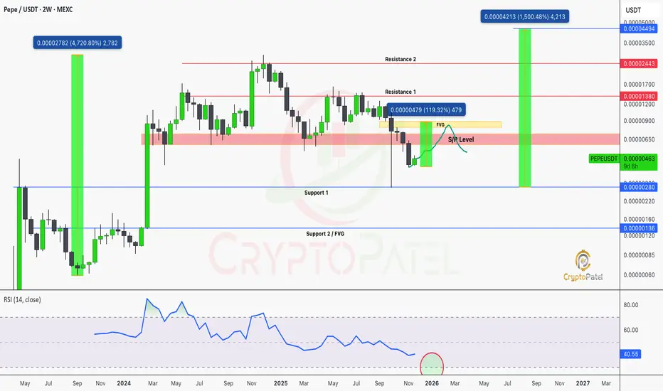
$PEPE Weekly Support Broken Or the Perfect Trap Before a Pump?CRYPTOCAP:PEPE Weekly Support Broken Or the Perfect Trap Before a Pump?
CRYPTOCAP:PEPE lost its weekly support and is now trading below it, which looks more like a full liquidity sweep than a real trend shift. I’m expecting a 50–100% relief rally before the next major move.
If key S/R flips and holds, we could see another memecoin cycle, with 1,000–1,500% upside back on the table.
Support / Accumulation: $0.00000280 / $0.00000136
Resistance / Targets: $0.00000914 → $0.00001380 → $0.00002443 → $0.00004494
Watch my levels closely before entering any trades.
NFA & DYOR
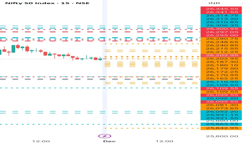
NIFTY- Intraday Levels - 1st December 2025If NIFTY sustain above 26202/12/15 above this bullish then around 26240/48 above more bullish around 26280 above this wait more levels marked on chart
If NIFTY sustain below 26187/62 below this bearish then 26110 support below this more bearish then 26099/95 strong level then very very strong level and last hope 26081/73 below this wait more levels marked on chart
My view :-
"My viewpoint, offered purely for analytical consideration, The trading thesis is: Nifty (bearish tactical approach: sell on rise)
This analysis is highly speculative and is not guaranteed to be accurate; therefore, the implementation of stringent risk controls is non-negotiable for mitigating trade risk."
Consider some buffer points in above levels.
Please do your due diligence before trading or investment.
**Disclaimer -
I am not a SEBI registered analyst or advisor. I does not represent or endorse the accuracy or reliability of any information, conversation, or content. Stock trading is inherently risky and the users agree to assume complete and full responsibility for the outcomes of all trading decisions that they make, including but not limited to loss of capital. None of these communications should be construed as an offer to buy or sell securities, nor advice to do so. The users understands and acknowledges that there is a very high risk involved in trading securities. By using this information, the user agrees that use of this information is entirely at their own risk.
Thank you.
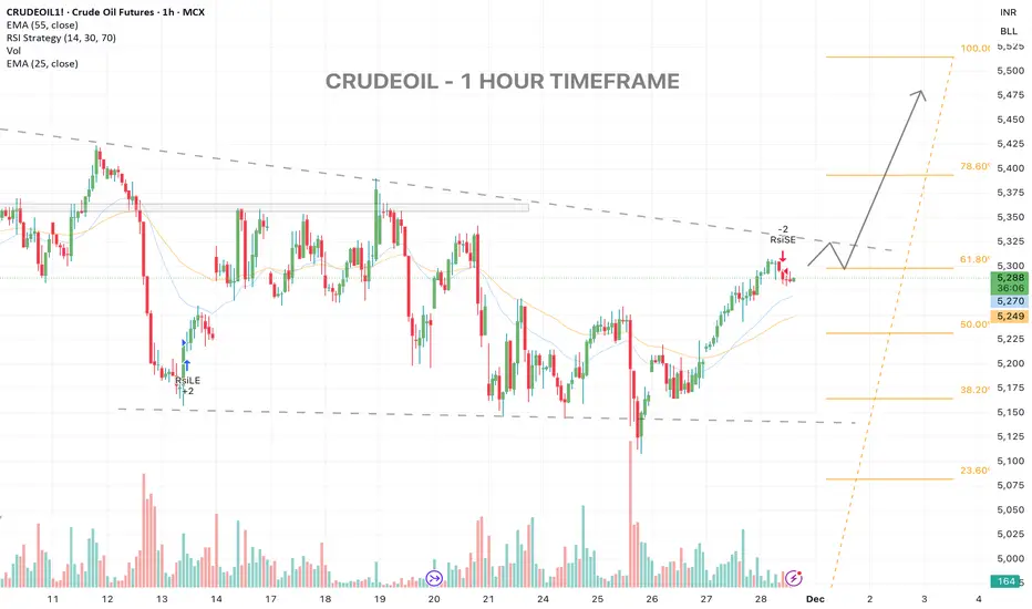
SOON BREAKOUT IN CRUDEOIL ?CRUDEOIL - 1 HOUR TIMEFRAME
Price is retesting the 61.8% zone right under the descending trendline.
A shallow pullback toward 5260–5275 can fuel the next leg toward 5335 / 5385 / 5450.
Overall, structure favors a continuation leg higher once the pullback stabilizes, remains bullish as long as 5205 holds. Watching for breakout confirmation.
Part 1 Intraday Trading Master ClassWhat Are Options?
Options are financial contracts that give you the right, but not the obligation, to buy or sell an underlying asset (like Nifty, Bank Nifty, a stock, etc.) at a fixed price within a specified time.
There are two types of options:
Call Option (CE) – Gives the right to buy
Put Option (PE) – Gives the right to sell
In India, all index and stock options are European style, which means they can be exercised only on expiry day, but they can be bought or sold (squared off) anytime before expiry.

PCR Trading Strategies How Option Prices Move (Option Greeks)
Option premiums move because of time, volatility, and market direction. The Greeks explain this movement.
1. Delta – Direction Sensitivity
Delta shows how much premium changes with a ₹1 move in the underlying.
Call delta: +0.3 to +1.0
Put delta: –0.3 to –1.0
Higher delta = faster premium movement.
2. Theta – Time Decay
Theta is the killer for option buyers.
As time passes, the premium loses value.
Sellers benefit from theta
Buyers suffer from theta
3. Vega – Volatility Impact
Higher volatility = higher option premiums.
Lower volatility = cheaper premiums.
4. Gamma – Acceleration of Delta
Gamma shows how fast delta changes.
Fast markets increase gamma dramatically.

Part 2 Master Candle Stick Patterns Key Terms in Options
Option trading revolves around certain essential terms that define risk, reward, and price movement.
Premium
The price you pay to buy an option.
For the buyer, premium = maximum loss.
Strike Price
The fixed level at which you buy (Call) or sell (Put) if you choose to exercise the contract.
Expiry
Every option expires weekly or monthly.
India has:
Weekly expiry: Nifty, Bank Nifty, Fin Nifty
Monthly expiry: All indices & stocks
