USDCAD | 1H Market Structure OutlookUSDCAD is currently trading within a well-defined short-term distribution range after engineering a strong impulsive rally from the late-January lows. The recent expansion into the 1.3700 handle appears to have tapped into a premium supply zone, where price printed rejection wicks, signaling the presence of institutional sell-side liquidity.
From an SMC / ICT perspective:
Price swept relative equal highs before showing displacement to the downside, hinting at a classic buy-side liquidity grab.
The rejection from the marked supply suggests smart money may be positioning for a retracement toward inefficiencies left below.
Internal structure is beginning to shift bearish on the lower timeframe, though confirmation would require a decisive break of structure (BOS) beneath the 1.3620 support.
Key Levels to Watch
Supply / Premium: 1.3695 to 1.3710
Intermediate Support: ~1.3620 (range floor)
Higher-Timeframe Demand: 1.3580 to 1.3600, aligning with the visible demand block and potential mitigation zone.
Projected Path
If price fails to reclaim the supply region, the probability favors a corrective move lower, potentially delivering a measured draw on liquidity into the demand zone. A brief pullback into a lower high followed by continuation would further validate bearish order flow.
Invalidation Scenario:
Sustained acceptance above 1.3710 would negate the bearish premise and open the door for continuation toward higher liquidity pools.
Bias: Short-term bearish while below supply, with expectations of liquidity engineering toward discounted pricing.
Trend Lines

Nifty 50 for 09 Feb 2026Important levels and trendlines for Nifty 50.
Disclaimer: This is for educational purposes only. Trading involves risk. Please consult with a SEBI-registered advisor before making any financial decisions.

Nifty Intraday Analysis for 06th February 2026NSE:NIFTY
Index has resistance near 25850 – 25900 range and if index crosses and sustains above this level then may reach near 26100 – 26150 range.
Nifty has immediate support near 25450 – 22400 range and if this support is broken then index may tank near 25200 – 25150 range.
The market has yet to decide whether the gap created on 3 February 2026—following developments in the India-US trade deal—will sustain or be filled.
Market sentiment will likely be driven by the RBI MPC meeting outcome tomorrow morning, as well as any announcements from the Iran-USA nuclear talks in Oman (scheduled for 11:30 IST).
If the Iran-USA Nuclear talk outcome is not announced during market hours or any unfavourable outcome, the market is expected to close lower.

Banknifty Intraday Analysis for 06th February 2026NSE:BANKNIFTY
Index has resistance near 60450 – 60550 range and if index crosses and sustains above this level then may reach near 60950 – 61050 range.
Banknifty has immediate support near 59650 - 59550 range and if this support is broken then index may tank near 59150 - 59050 range.
The market has yet to decide whether the gap created on 3 February 2026—following developments in the India-US trade deal—will sustain or be filled.
Market sentiment will likely be driven by the RBI MPC meeting outcome tomorrow morning, as well as any announcements from the Iran-USA nuclear talks in Oman (scheduled for 11:30 IST).
If the Iran-USA Nuclear talk outcome is not announced during market hours or any unfavourable outcome, the market is expected to close lower.

Finnifty Intraday Analysis for 06th February 2026 NSE:CNXFINANCE
Index has resistance near 27925 - 27975 range and if index crosses and sustains above this level then may reach near 28200 - 28250 range.
Finnifty has immediate support near 27475 – 27425 range and if this support is broken then index may tank near 26200 – 26150 range.
The market has yet to decide whether the gap created on 3 February 2026—following developments in the India-US trade deal—will sustain or be filled.
Market sentiment will likely be driven by the RBI MPC meeting outcome tomorrow morning, as well as any announcements from the Iran-USA nuclear talks in Oman (scheduled for 11:30 IST).
If the Iran-USA Nuclear talk outcome is not announced during market hours or any unfavourable outcome, the market is expected to close lower.

Midnifty Intraday Analysis for 06th February 2026NSE:NIFTY_MID_SELECT
Index has immediate resistance near 13825 – 13850 range and if index crosses and sustains above this level then may reach 13975 – 14000 range.
Midnifty has immediate support near 13575 – 13550 range and if this support is broken then index may tank near 13425 – 13400 range.
The market has yet to decide whether the gap created on 3 February 2026—following developments in the India-US trade deal—will sustain or be filled.
Market sentiment will likely be driven by the RBI MPC meeting outcome tomorrow morning, as well as any announcements from the Iran-USA nuclear talks in Oman (scheduled for 11:30 IST).
If the Iran-USA Nuclear talk outcome is not announced during market hours or any unfevaourable outcome, the market is expected to close lower.

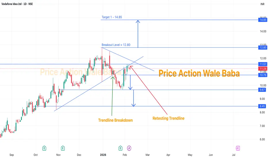
Vodafone - IdeaVodafone idea is the most trending stocks when comes to trading, because of small prices and movement.
Here, I have done some analysis of it and where you can find its trend.
1. Trend Understanding
- Vodafone idea was consolidating and then give the breakdown from rising channel or bearish flag.
- Then it had made a low of 9.68 and pull back to re-testing trendline.
- So, it is on trendline retesting and not going up.
2. Bearish Strategy
- So, what's now?? We should check if it will go down from here and again touch 9.68, then it will formed a head and shoulders pattern with neckline level 9.68.
- When it breaks 9.68 we can sell it for the target of 8.45.
3. Bullish Strategy
- Now, to see upside, we have to wait when it will breaks it high of 12.80.
- Once, it will breaks and sustain above 12.80, we will see target of 14.85 and more.
So, untill it can be sideways and consolidation in range of 12.80 and 9.68.
BankIndia - Rounding bottomBank of India has formed a rounding bottom pattern and also had a small breakout.
It had made high of 170 and then come down for the resting.
So, once it breaks and sustain above 170, you can buy and hold for the target of 200 and 220.
Buy on every dips after breakout, it will give handsome amount of return.

Nifty Intraday Analysis for 05th February 2026NSE:NIFTY
Index has resistance near 26050 – 26100 range and if index crosses and sustains above this level then may reach near 25325 – 25375 range.
Nifty has immediate support near 25550 – 22500 range and if this support is broken then index may tank near 25275 – 25225 range.
The market is yet to decide whether the gap created on 3rd February’26 amid India US trade deal development will sustain or be filled.

Banknifty Intraday Analysis for 05th February 2026NSE:BANKNIFTY
Index has resistance near 60650 – 60750 range and if index crosses and sustains above this level then may reach near 61150 – 61250 range.
Banknifty has immediate support near 59850 - 59750 range and if this support is broken then index may tank near 59350 - 59250 range.
The market is yet to decide whether the gap created on 3rd February’26 amid India US trade deal development will sustain or be filled.

Finnifty Intraday Analysis for 05th February 2026 NSE:CNXFINANCE
Index has resistance near 28025 - 28075 range and if index crosses and sustains above this level then may reach near 28300 - 28350 range.
Finnifty has immediate support near 27575 – 27525 range and if this support is broken then index may tank near 27300 – 27250 range.
The market is yet to decide whether the gap created on 3rd February’26 amid India US trade deal development will sustain or be filled.

Midnifty Intraday Analysis for 05th February 2026NSE:NIFTY_MID_SELECT
Index has immediate resistance near 13850 – 13875 range and if index crosses and sustains above this level then may reach 14000 – 14025 range.
Midnifty has immediate support near 13600 – 13575 range and if this support is broken then index may tank near 13450 – 13425 range.
The market is yet to decide whether the gap created on 3rd February’26 amid India US trade deal development will sustain or be filled.

ACC – Testing Major Multi-Year SupportACC is sitting at a crucial long-term support zone — a classic make-or-break level that could define the next major trend.
🔵 Bullish Case:
If support holds, wait for a strong weekly candle confirmation before considering longs. A solid bounce could drive price toward prior supply zones.
🔴 Bearish Case:
A decisive weekly close below support may trigger sharp downside. Watch for a break-and-retest for higher probability trades.
📌 View: This is a high-decision area. Stay patient and let the weekly timeframe confirm the move — the next breakout or breakdown could be powerful.

HAVELLS – Sitting at a Crucial Trendline Support✅ Bullish Scenario (Bounce Trade)
If the trendline holds, watch for a strong bullish confirmation such as a hammer or bullish engulfing candle with volume.
Trade Plan:
• Enter above the confirmation candle
• Stop Loss below the trendline
⚠️ Bearish Scenario (Breakdown Trade)
If price breaks the trendline decisively, avoid rushing into the trade.
Trade Plan:
• Wait for breakdown + pullback to the trendline
• Consider entry after rejection from the retest
• Stop Loss above the pullback high

Short Varun BeveragesStock is in Triangle.
Very High Chances of Breakdown.
Traingle is an Continuation Pattern. Previous Trend is Bearish to it will continue to go down.
450-460 is Resistance.
Chances of 350-390 levels on Chart.
Pattern invalid above 512

Part 1 Technical Analysis VS. Institutional Option Trading What Are Options?
Options are contracts that give you the right but not the obligation to buy or sell an asset at a fixed price before a certain date.
They are derivative instruments — their value comes from the underlying asset (index, stock, commodity, currency).
Options are mostly used for hedging, speculation, and income generation.
Two Types of Options
Call Option (CE): Right to buy at a chosen price.
Put Option (PE): Right to sell at a chosen price.

Volatility Index (VIX) Trading: Measuring Risk and Timing TradesWhat Is the Volatility Index (VIX)?
The VIX measures the market’s expectation of 30-day forward volatility derived from S&P 500 index option prices. Instead of tracking past price movements, it reflects implied volatility, meaning how much traders expect the market to fluctuate in the near future.
A low VIX suggests calm markets and investor confidence
A high VIX indicates fear, uncertainty, and elevated risk
Unlike price indices, the VIX is mean-reverting, meaning it tends to return to long-term average levels after extreme moves.
How the VIX Measures Risk
1. Market Sentiment Indicator
The VIX captures collective trader psychology. When investors rush to buy protective options (puts), implied volatility rises, pushing the VIX higher. This behavior often appears during:
Economic uncertainty
Geopolitical events
Financial crises
Sharp market sell-offs
Thus, the VIX becomes a real-time indicator of fear and risk aversion.
2. Risk Perception vs Actual Risk
Importantly, the VIX measures expected risk, not actual price movement. Markets can fall with a low VIX or rise with a high VIX. However:
Rising VIX + falling markets = confirmed risk escalation
Rising VIX + rising markets = instability beneath optimism
This distinction helps traders anticipate volatility expansions before price breakdowns occur.
Interpreting VIX Levels
Although exact levels vary over time, traders commonly interpret the VIX as follows:
Below 15 – Low volatility, complacency, bullish bias
15–20 – Normal volatility, balanced market
20–30 – Elevated risk, caution zone
Above 30 – High fear, panic conditions
Above 40 – Crisis or extreme uncertainty
Low VIX environments often precede sudden volatility spikes, while extremely high VIX levels frequently mark market bottoms.
VIX and Market Timing
1. VIX as a Contrarian Indicator
One of the most powerful uses of the VIX is contrarian trading. Extreme fear often occurs near market lows, while extreme calm often appears near market tops.
Very high VIX → potential buying opportunity in equities
Very low VIX → warning sign of overconfidence
This works because markets tend to overreact emotionally during extremes.
2. VIX Breakouts and Trend Changes
A sudden breakout in the VIX from a low base often signals:
Trend exhaustion
Incoming market correction
Transition from accumulation to distribution
Traders monitor VIX breakouts alongside:
Support/resistance on indices
Volume spikes
Market breadth deterioration
A rising VIX with weakening index structure often confirms trend reversal risk.
3. VIX Divergence Analysis
Divergences between the VIX and market indices provide early warning signals.
Bullish divergence: Market makes lower lows, VIX fails to make higher highs → selling pressure weakening
Bearish divergence: Market makes higher highs, VIX refuses to fall → hidden risk building
Such divergences are especially useful near major support or resistance levels.
Trading Strategies Using the VIX
1. Equity Market Confirmation Strategy
Traders use the VIX to confirm equity trades:
Long trades preferred when VIX is falling or stable
Short trades favored when VIX is rising sharply
Avoid aggressive longs during VIX spikes unless trading reversals
This approach helps filter false breakouts and low-probability setups.
2. Volatility Expansion and Contraction
Volatility moves in cycles:
Low volatility leads to high volatility
High volatility leads to low volatility
Traders anticipate expansion after prolonged quiet periods. Range-bound markets with a compressed VIX often precede:
Breakouts
Trend acceleration
News-driven moves
Recognizing these phases improves timing and position sizing.
3. Hedging with VIX Instruments
The VIX is widely used for portfolio hedging. During market stress:
Equity portfolios lose value
VIX instruments often gain
Professional traders hedge risk using:
VIX futures
VIX options
Volatility ETFs (with caution due to decay)
This strategy protects capital during sudden market shocks.
4. Options Trading and the VIX
For options traders, the VIX is critical:
High VIX → options expensive → prefer selling strategies
Low VIX → options cheap → prefer buying strategies
Using the VIX helps traders choose:
When to sell premium
When to buy volatility
Appropriate strike selection
Ignoring volatility often leads to poor risk-reward outcomes.
VIX and Risk Management
Position Sizing
When the VIX is elevated, price swings widen. Smart traders:
Reduce position size
Widen stop-losses
Avoid over-leveraging
Low VIX environments allow for:
Tighter stops
Higher leverage (with caution)
Adjusting size based on volatility keeps risk consistent.
Avoiding Emotional Trading
The VIX reflects collective fear, not just individual emotion. Watching it objectively helps traders:
Avoid panic selling
Stay disciplined during volatility spikes
Recognize when fear is excessive
This psychological edge is often more valuable than technical indicators alone.
Limitations of VIX Trading
While powerful, the VIX is not perfect:
It does not predict market direction
It is based on S&P 500 options, not all markets
Short-term VIX products suffer from decay
Sudden news can override signals
Therefore, the VIX should be used as a confirmation and risk tool, not a standalone system.
Conclusion
Volatility Index trading is less about predicting price and more about understanding risk, emotion, and timing. The VIX reveals what price charts often hide—market anxiety, complacency, and expectation. By integrating VIX analysis into trading strategies, traders gain a deeper awareness of when to be aggressive, when to protect capital, and when to wait.
Successful traders do not fight volatility—they read it, respect it, and trade around it. When used correctly, the VIX becomes not just a fear gauge, but a powerful compass for navigating uncertain markets.

Role of FII and DII in the Indian Stock MarketIntroduction
The Indian stock market is one of the fastest-growing capital markets in the world and attracts investments from both domestic and global participants. Among the most influential players in this ecosystem are Foreign Institutional Investors (FIIs) and Domestic Institutional Investors (DIIs). Their investment decisions significantly impact market direction, liquidity, volatility, and investor sentiment. Understanding the role of FIIs and DIIs is crucial for traders, long-term investors, policymakers, and anyone seeking to analyze market movements in India.
What are FIIs?
Foreign Institutional Investors (FIIs) are investment entities registered outside India that invest in Indian financial assets. These include:
Mutual funds
Pension funds
Hedge funds
Insurance companies
Sovereign wealth funds
Foreign portfolio investors (FPIs)
FIIs invest in equities, bonds, government securities, derivatives, and ETFs after registering with the Securities and Exchange Board of India (SEBI).
Key Characteristics of FIIs
Operate with large capital
Highly sensitive to global economic conditions
Often short- to medium-term focused
Move funds quickly across countries
Strong influence on benchmark indices like NIFTY 50 and Sensex
What are DIIs?
Domestic Institutional Investors (DIIs) are India-based institutions that invest in Indian financial markets. These include:
Mutual funds
Insurance companies (LIC, GIC)
Banks
Pension funds
Provident funds (EPFO, NPS)
DIIs represent domestic savings channeled into capital markets.
Key Characteristics of DIIs
Long-term investment horizon
More stable and less speculative
Influenced by domestic economic growth
Act as counter-balance to FIIs
Increasingly powerful due to SIP culture
Role of FIIs in the Indian Stock Market
1. Liquidity Provider
FIIs bring massive liquidity into Indian markets. Their large trade volumes:
Increase market depth
Reduce bid-ask spreads
Improve price discovery
High FII participation makes Indian markets more efficient and globally competitive.
2. Market Direction and Trend Formation
FII flows often decide market trends:
Net buying by FIIs → bullish markets
Net selling by FIIs → bearish or corrective markets
Sharp rallies and crashes are frequently linked to sudden FII inflows or outflows.
3. Impact on Blue-Chip Stocks
FIIs prefer:
Large-cap stocks
Index heavyweights
High-liquidity stocks
As a result, stocks like Reliance, HDFC Bank, Infosys, TCS, ICICI Bank are heavily influenced by FII activity.
4. Sensitivity to Global Factors
FIIs react strongly to:
US Federal Reserve interest rate decisions
Dollar strength or weakness
Global inflation data
Geopolitical tensions
Recession fears
This makes Indian markets sensitive to global news even if domestic fundamentals are strong.
5. Currency Impact
When FIIs invest:
They bring foreign currency → Rupee strengthens
When they exit:
Capital outflows → Rupee weakens
Thus, FII behavior directly impacts INR–USD exchange rates.
Role of DIIs in the Indian Stock Market
1. Market Stabilizers
DIIs act as a shock absorber during market downturns. When FIIs sell aggressively, DIIs often step in to buy, preventing deep crashes.
Example:
During global sell-offs, strong DII buying has helped Indian markets outperform peers.
2. Long-Term Wealth Creation
DIIs invest with a long-term vision aligned with:
India’s GDP growth
Corporate earnings
Demographic advantage
Their investments support sustainable wealth creation rather than short-term speculation.
3. Support from Retail Investors
The rise of:
SIPs (Systematic Investment Plans)
Mutual fund awareness
Digital investing platforms
has strengthened DIIs tremendously. Monthly SIP inflows provide consistent buying power even during volatile markets.
4. Reduced Dependence on Foreign Capital
As DII participation grows:
India becomes less vulnerable to sudden FII exits
Market volatility reduces
Financial independence increases
This shift is critical for long-term market stability.
5. Sectoral Impact
DIIs invest heavily in:
Banking and financial services
Infrastructure
FMCG
Manufacturing
PSU stocks
Their investments often align with national development priorities.
FII vs DII: Key Differences
Aspect FII DII
Origin Foreign Indian
Investment Horizon Short to medium Long term
Risk Appetite High Moderate
Sensitivity Global factors Domestic factors
Market Role Trend creator Trend stabilizer
Volatility Impact Increases volatility Reduces volatility
Interaction Between FIIs and DIIs
The Indian stock market often behaves like a tug-of-war between FIIs and DIIs.
When both buy → Strong bull market
When FIIs sell and DIIs buy → Sideways or controlled correction
When both sell → Sharp market crash
Understanding daily FII–DII data helps traders anticipate short-term market moves.
Impact on Retail Investors
Retail investors are indirectly influenced by FII and DII actions:
Rising FII inflows attract retail participation
DII buying builds confidence during corrections
Sharp FII selling can cause panic if not absorbed by DIIs
Smart investors track institutional flow data before making major decisions.
Regulatory Framework
SEBI closely monitors FII and DII activity to:
Prevent market manipulation
Ensure transparency
Maintain financial stability
Limits are placed on foreign ownership in certain sectors to protect national interests.
Importance for Traders and Investors
For Traders:
FII flow data helps in index trading
Short-term momentum often follows FII behavior
For Long-Term Investors:
DII accumulation signals confidence in fundamentals
Corrections caused by FII selling can offer buying opportunities
Conclusion
FIIs and DIIs are the backbone of the Indian stock market. FIIs bring global capital, liquidity, and momentum, while DIIs provide stability, long-term vision, and domestic strength. The growing influence of DIIs has made Indian markets more resilient and less dependent on foreign money.
For anyone serious about the Indian stock market, understanding the roles, behavior, and interaction of FIIs and DIIs is essential. Their combined actions shape market trends, influence valuations, and determine how India positions itself in the global financial landscape.

INDSWFTLAB - Volume increased at ResistanceDISCLAIMER: This is purely an observation and should not be considered a trade recommendation. Kindly conduct your own analysis before making any trading decisions.
Key Observations:
1. The price has repeatedly rejected the same level in previous attempts.
2. Currently, it is testing the strong resistance zone with notable volume.
3. A confirmed close of a strong bullish candle above the resistance zone is required for validation.

Nifty Intraday Analysis for 04th February 2026NSE:NIFTY
Index has resistance near 26000 – 26050 range and if index crosses and sustains above this level then may reach near 25275 – 25325 range.
Nifty has immediate support near 25500 – 22450 range and if this support is broken then index may tank near 25225 – 25175 range.
Expect continued volatility and swings until the India-US trade deal developments establish a new market base. It will be interesting to watch whether Gap created on 3rd February’26 will be respected in near term or filled by short traders.

Banknifty Intraday Analysis for 04th February 2026NSE:BANKNIFTY
Index has resistance near 60450 – 60550 range and if index crosses and sustains above this level then may reach near 60950 – 61050 range.
Banknifty has immediate support near 59650 - 59550 range and if this support is broken then index may tank near 59150 - 59050 range.
Expect continued volatility and swings until the India-US trade deal developments establish a new market base. It will be interesting to watch whether Gap created on 3rd February’26 will be respected in near term or filled by short traders.

Finnifty Intraday Analysis for 04th February 2026 NSE:CNXFINANCE
Index has resistance near 27900 - 27950 range and if index crosses and sustains above this level then may reach near 28175 - 28225 range.
Finnifty has immediate support near 27450 – 27400 range and if this support is broken then index may tank near 26175 – 26125 range.
Expect continued volatility and swings until the India-US trade deal developments establish a new market base. It will be interesting to watch whether Gap created on 3rd February’26 will be respected in near term or filled by short traders.

Midnifty Intraday Analysis for 04th February 2026NSE:NIFTY_MID_SELECT
Index has immediate resistance near 13775 – 13800 range and if index crosses and sustains above this level then may reach 13925 – 13950 range.
Midnifty has immediate support near 13525 – 13500 range and if this support is broken then index may tank near 13375 – 13350 range.
Expect continued volatility and swings until the India-US trade deal developments establish a new market base. It will be interesting to watch whether Gap created on 3rd February’26 will be respected in near term or filled by short traders.
