SPY - Hope it tops this time :)US markets have been super resilient, sucking capital from across the world.
We have a good pattern in place, as the triggers for pushing the market up have been reducing with time, with everything running quite thin.
The rally has been quite low on breadth and is supported on weak pillars - but still has been resilient and all selling have been bought into.
Let's see if it breaks and sustains this time.
We need a 10-15% (ideally + 20%) fall in US for money to flow into emerging markets :)
It is a good time to try some positional shorts with SL as 7k.
View void if we sustain above 7k.
Wave Analysis

#Nifty Directions and Levels for Jan 12thGood morning, friends! 🌞
Market Directions and Levels for Jan 12th
Global remains positive, though Indian markets show a bearish bias. Today, the market may open neutral to slightly gap down, as GIFT Nifty trades about 20 points lower.
Current View
> If the market declines initially, the immediate support zone is expected to act as a strong support.
> If price gets rejected from this zone, structurally this could be a 5th sub-wave. In that case, the 5th sub-wave correction may complete here, followed by a bounce of around 38%–61% of the minor swing.
> This is the base structure. However, if price does not reject around the pullback zone, the 5th sub-wave could extend toward 25,550–25,580 for Nifty.
Alternate View
> The alternate scenario suggests a range-bound market with a bearish bias.
> If the market opens positive, we can expect a bounce of around 23%–38%. However, even if a bounce occurs, the broader outlook remains bearish, and the market may return to its opening level by the end of the day.

NIFTY Forms Ending Diagonal (EDT): 25,133–25,000 final Target.✅ STRUCTURE CONFIRMATION
1️⃣ Impulse completed
✔ NIFTY has completed a 5-wave impulse as per the chart
✔ Wave (v) showed:
Overlap
Momentum divergence
Channel resistance
➡️ This strongly suggests an Ending Diagonal–type Wave (v), which often leads to sharp ABC corrections
2️⃣ Current phase: ABC correction in progress
Your ABC expectation is correct.
🔹 Wave A
Sharp decline from the top
Impulsive nature ✔
🔹 Wave B (ongoing / upcoming)
Counter-trend bounce
Overlapping, corrective
Lower volume
📌 Important:
👉 Any Wave-B bounce is a shorting opportunity, not a trend resumption
Ideal Wave-B retracement zone:
25,800 – 26,000
Near broken channel / prior resistance
3️⃣ Wave C termination zone (KEY POINT)
Your final buy zone is well identified.
🎯 High-probability Wave-C completion:
25,133 – 25,000
Why this zone matters:
✔ 200-EMA (~25,133)
✔ Ending Diagonal trendline (EDT) support
✔ 50–61.8% Fibonacci retracement
✔ Prior demand + institutional reference level
📌 This is a confluence zone, which is exactly where Elliott Wave corrections typically end.
4️⃣ Trading logic (very clear)
❌ Do NOT buy during Wave B
✅ Use Wave-B rallies to sell / hedge
✅ Final buy should be planned near 25,133 ± 150 pts
Expect volatility and false breakdowns near the bottom
5️⃣ Invalidation (must know)
❌ Weekly close below 24,600
Would imply a deeper, higher-degree correction
Until then → bullish structure intact

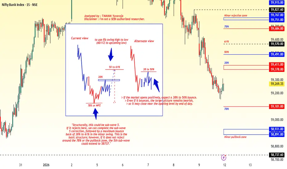
#Banknifty Directions and Levels for Jan 12thCurrent View
> If the market declines initially, the immediate support zone is expected to act as a strong support.
> If price gets rejected from this zone, structurally this could be a 5th sub-wave. In that case, the 5th sub-wave correction may complete here, followed by a bounce of around 38%–61% of the minor swing.
> This is the base structure. However, if price does not reject around the pullback zone, the 5th sub-wave could extend toward 58,737.
Alternate View
> The alternate scenario suggests a range-bound market with a bearish bias.
> If the market opens positive, we can expect a bounce of around 23%–38%. However, even if a bounce occurs, the broader outlook remains bearish, and the market may return to its opening level by the end of the day.
[INTRADAY] #BANKNIFTY PE & CE Levels(12/01/2026)A flat opening is expected in Bank Nifty, with the index continuing to trade within the same downward structure seen over the last few sessions. Price is currently hovering around the 59,250–59,300 zone, which is acting as an intraday equilibrium area where minor pullbacks and short-covering are visible, but no strong buying conviction has emerged yet. Overall sentiment remains cautious unless a clear breakout occurs.
On the upside, a sustained move above 59,550 will be the key trigger for bullish momentum. If Bank Nifty manages to hold above this level, long trades / CE positions can be considered with upside targets at 59,750, 59,850, and 59,950+. A clean breakout above 59,950 may further open the gates toward higher resistance zones.
On the downside, if the index fails to hold 59,250–59,200, selling pressure may intensify. In such a scenario, PE positions can be considered with downside targets at 59,050, 58,950, and 58,750. A decisive breakdown below 58,950 could extend the move toward 58,650 and 58,550-. Until a clear directional move is confirmed, traders are advised to stick to level-based trades with strict risk management and avoid aggressive positions.

NIFTY : Trading levels and Plan for 12-Jan-2026(Timeframe: 15-min | Gap criteria considered: 100+ points)
🔑 Key Levels (from chart)
Last Intraday Resistance: 25,998
Opening Resistance Zone: 25,742 – 25,816
Spot / Pivot Area: 25,700
Opening Support Zone: 25,592 – 25,647
Last Intraday Support: 25,353
🧠 Market structure note: NIFTY is in a short-term downtrend, but currently showing a relief bounce from demand. Price is approaching an important supply zone, where rejection risk remains high unless acceptance improves.
🟢 1. GAP-UP OPENING (100+ Points)
If NIFTY opens above 25,742, it will be a pullback rally into resistance.
🎓 Educational Insight
Gap-ups in a corrective downtrend often face selling near supply zones. Strength is confirmed only when price holds above resistance, not just spikes.
Plan of Action
Avoid aggressive longs in the first 15 minutes ⏳
Sustain above 25,816 → move toward 25,998
Rejection from 25,742 – 25,816 → pullback toward 25,700
Fresh longs only after retest + higher low
Options idea: Bull Call Spread (ATM buy + OTM sell)
🟡 2. FLAT OPENING
If NIFTY opens near 25,680 – 25,720, expect range-bound and volatile price action.
🎓 Educational Insight
Flat opens near VWAP / pivot after a sell-off usually result in false breakouts. Direction emerges only after range expansion with volume.
Plan of Action
Above 25,742 → upside toward 25,816
Failure above 25,742 → sideways to weak bias
Break below 25,592 → selling toward 25,353
Avoid trades inside the middle range 🚫
Options idea: Iron Fly / Short Strangle with hedge
🔴 3. GAP-DOWN OPENING (100+ Points)
If NIFTY opens below 25,592, bears remain firmly in control.
🎓 Educational Insight
Gap-downs into demand can cause short covering bounces, but continuation happens if price fails to reclaim the opening range.
Plan of Action
First support to watch: 25,592 – 25,647
Weak bounce + rejection → downside toward 25,353
Sustain below 25,353 → further trend continuation
Avoid fresh shorts exactly at support
Options idea: Bear Put Spread / Put Debit Spread
🛡️ Risk Management Tips (Options Trading)
Risk only 1–2% capital per trade 💰
Prefer spreads over naked buying in volatile zones
Book partial profits at resistance/support levels
No averaging against the trend 🚫
Stop trading after 2 consecutive losses 🧠
🧾 Summary & Conclusion
Above 25,816: Relief rally toward 25,998
25,742 – 25,816: Selling / supply zone
Below 25,592: Weakness toward 25,353
Focus on price acceptance, not prediction 🎯
⚠️ Disclaimer
I am not a SEBI-registered analyst. This trading plan is for educational purposes only. Markets are risky, and I may be wrong. Please consult a qualified financial advisor before taking trades.

Weekly Timeframe Price Action MasteryObserve the red supply zone where price consistently faces resistance, halting upward moves with precision. The green demand zone, formed after a decisive breakout from prior resistance, now acts as robust support for subsequent bounces. The white counter trend line serves as the pattern's key action line, guiding price movements with remarkable adherence across multiple tests.
Zone Dynamics
Supply zones in red mark areas of overhead selling pressure on weekly charts, often leading to rejections. Demand zones in green emerge post-breakout when former resistance flips, attracting buyers on retracements. These zones filter noise effectively in trending markets.
Counter Trend Line Role
This white line defines the counter-trend structure, respected through pullbacks and rallies. Price follows it as a dynamic guide, confirming pattern integrity without implying direction. Such lines enhance zone analysis by highlighting momentum shifts.
Disclaimer
This post showcases historical price action only and constitutes neither financial advice nor trading signals. Trading involves substantial risk of loss; conduct your own analysis and consult professionals.

ABCapital -> A Clear opportunity.Currently playing larger wave 3.
Played all earlier sub waves perfectly.
Currently playing sub wave C of 4 of 5 of 3.
Well aligned with fib ratio's.
Also clear divergence in RSI.
Minimum target of 335/-(Around 5%) is very much possible in short term.

Part 4 Learn Institutional Trading What Are Options?
At its core, an option is a financial derivative contract that gives the buyer the right, but not the obligation, to buy or sell an underlying asset at a predetermined price (known as the strike price) on or before a specific date (the expiration date). Unlike buying the asset outright, purchasing an option requires paying a premium, which is the cost of acquiring the right conveyed by the option.
Options are broadly classified into two types:
Call Option: Gives the holder the right to buy the underlying asset at the strike price.
Put Option: Gives the holder the right to sell the underlying asset at the strike price.

BEL- Wave 4 playing, Triangle FormationGood shorting candidate. Wave E of triangle starts playing now ...Wave B top can be used as a strict stoploss.
Wait for a confirmation Candle before taking position.
RSI is well within 70

BUY BABY CHART ANALYSIS Buy and hodl for some time swing trade for 1 day candlestick pattern chart analysis its lowesr our 1 day all liquidation grab and this is tha demand and buy in partial ohk its only my analysis buy at your own risk

Unlock Market Rotation: Turn Shifting Trends into Powerful ProfiStay Ahead of Capital Flow & Capture the Next Big Opportunity
What Is Market Rotation?
Market rotation refers to the movement of capital from one sector, asset class, or investment theme to another as economic conditions, interest rates, inflation, and growth expectations change. Understanding this shift allows investors to align portfolios with where money is flowing next, not where it has already been.
Why Market Rotation Matters More Than Ever
In today’s fast-moving global markets, leadership changes quickly. Sectors that outperform in one phase of the cycle can underperform in the next. Investors who unlock market rotation gain a powerful edge by identifying early signals and positioning before the crowd reacts.
Economic Cycles Drive Rotation
Different sectors perform best at different stages of the economic cycle. Early recovery favors cyclicals, mid-cycle supports growth sectors, late-cycle shifts toward defensives, and slowdown phases reward capital preservation strategies. Market rotation is the bridge between macro trends and smart allocation.
Interest Rates as a Key Trigger
Rising interest rates often rotate money away from high-growth, high-valuation stocks toward value, financials, and commodities. Falling rates usually support technology, consumption, and growth-oriented sectors. Tracking rate expectations is critical to anticipating rotation.
Inflation and Sector Leadership
Inflation reshapes winners and losers. High inflation typically benefits energy, metals, and real assets, while compressing margins in rate-sensitive sectors. Unlocking rotation means understanding how inflation impacts pricing power across industries.
Institutional Money Leaves Clues
FIIs, DIIs, and large institutional players move capital systematically. Volume expansion, relative strength, and sectoral index breakouts often signal early institutional rotation. Smart investors learn to read these footprints rather than react to headlines.
Relative Strength Is the Core Tool
Market rotation is best identified through relative performance. Comparing sectors against benchmark indices reveals which areas are gaining strength and which are losing momentum. Sustained outperformance is a strong sign of rotation in progress.
From Sector to Stock-Level Rotation
Rotation doesn’t stop at sectors—it flows into sub-sectors and then into specific stocks. Leaders within a strong sector usually outperform peers. Unlocking market rotation means narrowing focus from macro to micro with precision.
Risk Management Through Rotation
Instead of exiting markets entirely, rotation allows investors to shift risk, not abandon opportunity. When one theme weakens, another strengthens. This approach smooths volatility and improves long-term consistency.
Psychology of Market Rotation
Most investors chase past performance. Market rotation rewards those who act before trends become obvious. Discipline, data-driven decisions, and patience are essential to avoid emotional investing.
Technical Indicators That Signal Rotation
Moving averages, sectoral relative strength lines, momentum oscillators, and trend confirmation tools help validate rotation. Technical confirmation ensures that allocation decisions are backed by price action, not assumptions.
Macro Events Accelerate Rotation
Central bank decisions, geopolitical shifts, policy reforms, and global growth changes can rapidly accelerate capital movement. Prepared investors use these events as catalysts rather than shocks.
Short-Term vs Long-Term Rotation
Rotation can be tactical (weeks to months) or strategic (quarters to years). Traders benefit from short-term sector momentum, while investors focus on structural shifts like digitization, energy transition, or infrastructure growth.
Equity, Debt, and Alternative Rotation
Rotation is not limited to equities. Capital also moves between stocks, bonds, commodities, and alternative assets. A holistic approach captures opportunities across asset classes.
Market Rotation in Indian Markets
In India, rotation often reflects domestic growth cycles, government policies, earnings visibility, and global capital flows. Understanding local drivers adds a significant advantage to portfolio positioning.
Avoiding Overcrowded Trades
When a sector becomes over-owned, upside potential reduces. Unlocking market rotation helps investors exit crowded themes early and enter emerging ones before valuations expand.
Consistency Beats Prediction
Market rotation is not about predicting tops or bottoms. It is about consistently reallocating capital toward strength and away from weakness based on objective signals.
Portfolio Rebalancing with Purpose
Regular rebalancing aligned with rotation trends keeps portfolios dynamic. This reduces drawdowns and improves risk-adjusted returns over time.
Long-Term Wealth Creation Advantage
Investors who master market rotation compound gains by riding multiple leadership cycles instead of staying stuck in one theme. This adaptability is key to sustainable wealth creation.
Unlock the Edge
Market rotation is the silent force behind every major rally and correction. Those who understand it move ahead of trends, protect capital during uncertainty, and capture opportunity when it matters most.
Unlock Market Rotation is not just a strategy—it’s a mindset. By tracking capital flow, aligning with economic cycles, and acting decisively, investors can transform uncertainty into opportunity and stay one step ahead of the market.

Understanding Rapid Price Movements Through Technical AnalysisTechnical Market Explosion:
A technical market explosion refers to a sudden, powerful, and often unexpected surge in price movement—either upward or downward—driven primarily by technical factors rather than immediate fundamental news. These explosive moves are commonly observed across equities, commodities, forex, and cryptocurrencies and are closely followed by traders because they often create high-profit opportunities within short time frames. Understanding why and how these explosions occur is essential for traders and investors who rely on technical analysis to navigate volatile markets.
1. Meaning of a Technical Market Explosion
A technical market explosion occurs when price action breaks out decisively from a consolidation zone, key resistance, or support level with strong momentum and volume. This move is usually rapid and sharp, leaving little time for indecision. Such explosions reflect a sudden shift in market psychology where buyers or sellers overwhelm the opposing side.
These movements are not random; they are often the result of prolonged price compression, accumulation, or distribution phases that eventually release stored market energy.
2. Role of Support and Resistance Breakouts
Support and resistance levels are the backbone of technical analysis. A technical explosion typically begins when price decisively breaks above resistance or below support. Traders place buy stops above resistance and sell stops below support, and when these levels are breached, a cascade of orders is triggered.
This chain reaction increases liquidity and momentum, accelerating price movement. The stronger and more tested the level, the more explosive the breakout tends to be when it finally occurs.
3. Volume as the Fuel of Explosion
Volume plays a crucial role in validating a technical market explosion. A genuine breakout is almost always accompanied by a sharp rise in volume, signaling strong participation by institutional and retail traders.
Low-volume breakouts often fail, while high-volume explosions suggest conviction and sustainability. Volume confirms that the move is supported by real money, not just speculative noise.
4. Volatility Compression and Expansion
Before a market explodes, volatility usually contracts. This phase is marked by narrow price ranges, tight Bollinger Bands, or triangle and wedge formations. Such patterns indicate indecision and balance between buyers and sellers.
When volatility expands suddenly, it signals the start of a technical explosion. Traders who recognize volatility compression early can position themselves ahead of the breakout.
5. Indicator Alignment and Momentum
Technical indicators often align before a market explosion. Momentum indicators like RSI, MACD, and Stochastic Oscillators show strength or divergence prior to the move. For example:
RSI holding above 50 indicates bullish strength
MACD bullish crossover near zero line signals momentum buildup
Moving averages start flattening or converging before expansion
When these indicators turn simultaneously, the probability of an explosive move increases.
6. Chart Patterns Triggering Explosions
Certain chart patterns are well known for leading to technical market explosions, including:
Ascending and descending triangles
Cup and handle patterns
Flags and pennants
Head and shoulders (especially breakdowns)
These patterns represent structured market behavior, and once their boundaries are violated, price often moves swiftly toward projected targets.
7. Institutional Activity and Smart Money
Institutional players often accumulate positions quietly during consolidation phases. This accumulation is not obvious to most traders but can be detected through price structure and volume behavior.
Once institutions complete accumulation or distribution, they allow price to move aggressively. This is when retail traders observe a technical market explosion, often entering late but still benefiting from momentum.
8. Role of Algorithmic and High-Frequency Trading
In modern markets, algorithmic trading plays a major role in accelerating technical explosions. Algorithms are programmed to react instantly to technical signals such as breakouts, moving average crossovers, and volatility spikes.
When a key level breaks, thousands of automated orders execute simultaneously, intensifying the speed and magnitude of the move.
9. False Breakouts vs True Explosions
Not every breakout leads to a true explosion. False breakouts occur when price briefly moves beyond a key level but lacks volume or follow-through. Recognizing the difference is critical.
True technical explosions show:
Strong closing prices beyond the breakout level
Increasing volume
Momentum continuation across multiple candles
False moves often retrace quickly and trap impatient traders.
10. Risk Management During Explosive Moves
While technical market explosions offer high reward, they also carry high risk. Rapid price movement can lead to slippage and emotional decision-making.
Effective risk management includes:
Predefined stop-loss levels
Position sizing based on volatility
Avoiding over-leverage
Waiting for candle confirmation instead of chasing price
Discipline is essential to survive and profit consistently from explosive markets.
11. Psychological Impact on Traders
Explosive moves create fear and greed simultaneously. Traders who miss the initial move feel fear of missing out (FOMO), while those in profit may panic and exit early.
Professional traders remain calm, follow their strategy, and understand that technical explosions are part of a broader market cycle, not isolated events.
12. Timeframe Perspective
Technical market explosions occur across all timeframes. On lower timeframes, they may last minutes or hours, while on higher timeframes, they can develop into long-term trends lasting months or years.
Swing traders, day traders, and investors interpret explosions differently, but the underlying technical principles remain the same.
13. Post-Explosion Behavior
After an explosive move, markets often pause, consolidate, or retrace partially. This phase is healthy and allows new participants to enter.
Strong markets use post-explosion consolidation as a base for the next leg, while weak markets fail to hold gains and reverse.
Conclusion
A technical market explosion is the result of accumulated market energy released through key technical triggers such as breakouts, volume surges, indicator alignment, and volatility expansion. These moves reflect shifts in market psychology and institutional participation rather than pure randomness.
For traders who master technical analysis, recognizing early signs of an impending explosion can provide significant opportunities. However, success depends not only on identifying the move but also on managing risk, controlling emotions, and respecting market structure. In fast-moving markets, preparation—not prediction—is the true edge.

RELIANCE may head for 1111 #RELIANCE is forming a NEAT 3-3-5 FLAT and should head for 1111. Anybody in EW kindly study and share views. In simple terms if you see the two DTF and WTF charts , the stock is forming a 3-3-5 FLAT correction STARTING 12 July 2024 where sub wave -a has three sub waves culminating at 1114 on 07 Apr 2025 and sub sub -c of this wave is ending as a 5 wave Ending Diagonal. Then we have sub wave-b going up in three sub waves again culminating at 1611 high on 03 Jan 2026. Now I am looking for sub wave -c going deep down to 1111 in five sub waves 1-2-3-4-5 as I have shown in the DTF Chart. ANALYSIS INVALIDATION 1611 ( or even 1575 may be good enough for invalidation). THIS DTF CHART ( Daily Time Frame).Lets C

#RELIANCE at 1475 heading for 1111 in 3-3-5 Elliott Wave FLAT #RELIANCE at 1475 is forming a NEAT 3-3-5 FLAT and should head for 1111. Anybody in EW kindly study and share views. In simple terms if you see the two DTF and WTF charts , the stock is forming a 3-3-5 FLAT correction STARTING 12 July 2024 where sub wave -a has three sub waves culminating at 1114 on 07 Apr 2025 and sub sub -c of this wave is ending as a 5 wave Ending Diagonal. Then we have sub wave-b going up in three sub waves again culminating at 1611 high on 03 Jan 2026. Now I am looking for sub wave -c going deep down to 1111 in five sub waves 1-2-3-4-5 as I have shown in the DTF Chart. ANALYSIS INVALIDATION 1611 ( or even 1575 may be good enough for invalidation). Lets C

Catostrophic time aheadDear Humans,
I have a strange finding about the coming time which is going to be tougher than 2008, yes its 100years cycle and we are going to see repeat of 1929-1931, I have marked the fall in RED in WXYXZ style move, market always gives you one chance and we are still adamant on on upward direction and investing at top levels where smart money is selling quiet Easily....
Nifty doesn't have any charts or exchange was not there during this time while we can see in Dow john's chart.
the current scenario at ground levels is that even a Lower and medium class is suffering because of the money scarcity in the market..
I can see that we are going to fall around 78%(precisely 76.4%) from highs by may 2027 in just one and half years time as we are in era of social media where movements are very fast ,,1929-1931 was 2.5 years time great depression.. " what name the market will it be given to this Catastrophic fall" ..
those who were mongeringfall of 12500 levels pre covid high levels at 16000/18000/20000/23500, its time to see those levels again, yes by May/June 2026 . unfortunately they all became bulls now and talking of 28000-30000 levels. well the investor has to hold on for 6 years or more to see these levels again, as history suggest that once such brutal fall happens then time takes its own course to rise again.
even Astro is suggesting Jupiter in 6/8 axis and malific ketu during this 6 years so the journey will be tough to rise from 6000 levels .. so its a time and price fall this time, both together..
Great Depression / Recession/ stagflation/WW3 god knows what all we see ? but
chart is showing a horrific picture..
Its a bigger time frame fall ( weekly, monthly & Yearly) so post this destruction we will not see these brutal levels for next bigger cycle atleast.. may God gives energy & courage to face the tough time coming ahead..
Yes after this fall we will enter into big time bull ERA, Prosperity, growth and growth only..
This post will really help next to next generations to see this interesting finding, if this software pertains that time..
* disclaimer:
its my personal finding for education purpose only and don't take any trade on basis of this.

Short term Analysis of HDFC BankWrap up:-
HDFC Bank is making a wxy pattern in wave c and has completed its wave w at 1018 and wave x is completed at 933. Thereafter, HDFC Bank will head towards wave y.
What I’m Watching for 🔍
Buy HDFC Bank @933 sl 927 for a target of 1027-1078.
Disclaimer: Sharing my personal view — only for educational purpose not financial advice.
"Don't predict the market. Decode them."

Real Knowledge of Candle patterns Candlestick patterns reflect the most important element in trading—market psychology and momentum. Each candle represents:
Open price
High
Low
Close
Candles show emotions like greed, fear, indecision, manipulation, and momentum.
Candlestick patterns can be categorized as:
1. Reversal Patterns
2. Continuation Patterns
3. Indecision Patterns
1. Reversal Candlestick Patterns
-Bullish Reversal Patterns
Hammer
Morning Star
Bullish Engulfing
Piercing Line
Dragonfly Doji
-Bearish Reversal Patterns
Shooting Star
Evening Star
Bearish Engulfing
Dark Cloud Cover
Gravestone Doji

STEELCAS 1 Day Time Frame 📊 Current Price Snapshot (Latest Available)
Approx Live Price: ~₹210–₹213 per share (recent session)
Today’s Day Range (recent close): ~₹208–₹214
📈 Accurate Daily Support & Resistance Levels
🔹 Pivot Point (Day Reference)
Pivot: ~₹206.55–₹213.62 (central reference)
📉 Support Levels
S1: ~₹203.7–₹205.8 – first key support
S2: ~₹197.1–₹201.1 – stronger secondary support
S3: ~₹188.8–₹193.3 – deep support zone
📈 Resistance Levels
R1: ~₹218.5–₹218.3 – first resistance
R2: ~₹226.8–₹226.1 – next upside target
R3: ~₹233.4–₹230.7 – higher resistance
🧠 How to Use These Levels (Daily Time Frame)
Bullish scenario
Break and hold above R1 (~₹218–219) could signal continuation toward R2 (~₹226+).
Sustained break above R2 strengthens trend.
Bearish scenario
Failure under Pivot (~₹206–213) with close below S1 (~₹204–206) may open S2 (~₹197) and S3 (~₹188).
Look for volume confirmation on breakdowns.
📍 Quick Reference Summary (Daily Levels)
Level Price Approx
R3 ~₹230–₹233+
R2 ~₹226–₹227
R1 ~₹218–₹219
Pivot ~₹206–₹213
S1 ~₹203–₹206
S2 ~₹197–₹201
S3 ~₹188–₹193

Crypto Investing Guide: Roadmap to Digital Asset InvestingCryptocurrency investing has evolved from a niche technological experiment into a global financial phenomenon. With Bitcoin, Ethereum, and thousands of alternative digital assets now traded worldwide, crypto has attracted retail investors, institutions, and even governments. However, crypto investing is fundamentally different from traditional investing due to its high volatility, emerging technology, regulatory uncertainty, and unique market dynamics. This guide provides a comprehensive overview of crypto investing, covering fundamentals, strategies, risks, and best practices to help investors make informed decisions.
Understanding Cryptocurrency and Blockchain
At its core, cryptocurrency is a digital or virtual currency secured by cryptography and typically built on blockchain technology. A blockchain is a decentralized, distributed ledger that records transactions across a network of computers. Unlike traditional financial systems controlled by central authorities, blockchains operate on consensus mechanisms such as Proof of Work (PoW) or Proof of Stake (PoS). This decentralization is a key value proposition, offering transparency, immutability, and resistance to censorship.
Bitcoin, the first cryptocurrency, was designed as a peer-to-peer electronic cash system. Ethereum expanded the concept by enabling smart contracts—self-executing programs that run on the blockchain—paving the way for decentralized finance (DeFi), non-fungible tokens (NFTs), and Web3 applications. Understanding these technological foundations is essential before investing, as the value of crypto assets is often tied to their utility, network adoption, and security.
Types of Crypto Assets
Crypto assets can be broadly categorized into several groups. Payment coins like Bitcoin and Litecoin focus on value transfer and store of value. Platform tokens such as Ethereum, Solana, and Avalanche support decentralized applications. Utility tokens grant access to specific services within an ecosystem. Stablecoins are pegged to fiat currencies and aim to reduce volatility. Governance tokens allow holders to vote on protocol decisions. Each category carries different risk and return profiles, making diversification across types an important consideration.
Why People Invest in Crypto
Investors are drawn to crypto for multiple reasons. Some view it as a hedge against inflation and currency devaluation, especially in economies with unstable monetary systems. Others are attracted by the potential for high returns, as early adopters of successful projects have historically seen significant gains. Additionally, crypto offers exposure to cutting-edge innovation in finance, technology, and digital ownership. However, these opportunities come with heightened risks that require careful evaluation.
Investment Strategies in Crypto
Crypto investing strategies range from conservative to highly speculative. Long-term investing (HODLing) involves buying fundamentally strong projects and holding them through market cycles, betting on long-term adoption. Dollar-cost averaging (DCA) reduces timing risk by investing fixed amounts at regular intervals. Active trading focuses on short-term price movements using technical analysis but requires experience, discipline, and risk management. Staking and yield farming allow investors to earn passive income by locking assets in networks or DeFi protocols, though they introduce smart contract and liquidity risks.
A disciplined strategy should align with the investor’s risk tolerance, time horizon, and financial goals. Overexposure to a single asset or strategy can significantly increase downside risk.
Fundamental and Technical Analysis
Successful crypto investing relies on analysis. Fundamental analysis examines factors such as the project’s use case, team, tokenomics, roadmap, community support, and real-world adoption. Metrics like active addresses, transaction volume, and total value locked (TVL) provide insights into network health. Technical analysis, on the other hand, studies price charts, trends, support and resistance levels, and indicators like RSI or moving averages to identify potential entry and exit points. Combining both approaches can lead to more balanced decisions.
Risk Management and Volatility
Crypto markets are notoriously volatile, with prices capable of swinging dramatically in short periods. Risk management is therefore critical. Investors should never invest money they cannot afford to lose, use position sizing to limit exposure, and avoid excessive leverage. Setting stop-loss levels, maintaining diversification, and periodically rebalancing portfolios can help manage downside risk. Emotional discipline is equally important, as fear and greed often drive poor decisions during extreme market moves.
Security and Storage
Security is a unique concern in crypto investing. Assets are controlled by private keys, and losing them can mean permanent loss of funds. Investors can store crypto on exchanges, software wallets, or hardware wallets. While exchanges offer convenience, they carry counterparty risk. Hardware wallets provide higher security for long-term holdings. Practicing good security hygiene—such as enabling two-factor authentication, avoiding phishing links, and backing up recovery phrases—is essential.
Regulation and Taxation
Crypto regulations vary widely across countries and are constantly evolving. Some jurisdictions embrace digital assets, while others impose restrictions or bans. Investors must stay informed about local regulations, compliance requirements, and tax obligations. Profits from crypto trading are often subject to capital gains tax, and improper reporting can lead to legal issues. Regulatory clarity can significantly impact market sentiment and asset prices.
Common Mistakes to Avoid
New investors often fall into predictable traps: chasing hype, investing without research, overtrading, or relying solely on social media tips. Another common mistake is ignoring fees, liquidity, and security risks. Patience, education, and a long-term perspective can help avoid costly errors.
Conclusion
Crypto investing offers unique opportunities to participate in a rapidly evolving digital economy, but it is not a guaranteed path to wealth. Success requires a solid understanding of blockchain technology, thoughtful strategy selection, disciplined risk management, and continuous learning. By approaching crypto with a balanced mindset—embracing innovation while respecting risk—investors can navigate this dynamic market more effectively and build a resilient digital asset portfolio over time.

Major Crash Ahead?The Diametric Pattern completed.
2-stage confirmation achieved.
The Major impulsive downtrend has begun - Unless there is a sharp reversal upside by next week.

XAUUSD Beginning Big Elliot Wave 3based on elliot waves counting on the daily timeframe we are currently in wave 2 pullback.
if we have seen the bottom of wave 2 already, the next wave is going to be the big impulse wave 3, with target marked on the chart below.
TLD: Long

What exactly you have to do when the Markets are REDI make educational content videos for swing trading basis
Charts used are older than 3 months in this video
