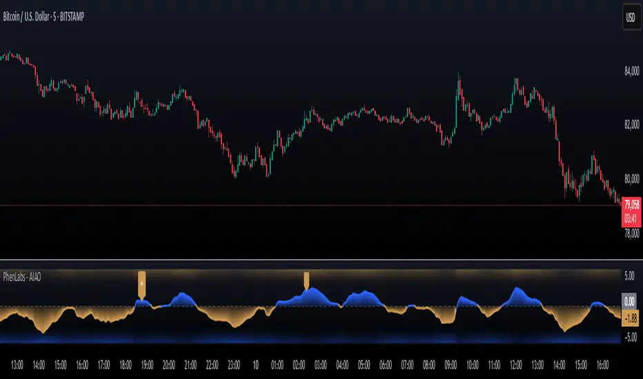
AI Adaptive Oscillator [PhenLabs]📊 Algorithmic Adaptive Oscillator
Version: PineScript™ v6
📌 Description
The AI Adaptive Oscillator is a sophisticated technical indicator that employs ensemble learning and adaptive weighting techniques to analyze market conditions. This innovative oscillator combines multiple traditional technical indicators through an AI-driven approach that continuously evaluates and adjusts component weights based on historical performance. By integrating statistical modeling with machine learning principles, the indicator adapts to changing market dynamics, providing traders with a responsive and reliable tool for market analysis.
🚀 Points of Innovation:
Ensemble learning framework with adaptive component weighting
Performance-based scoring system using directional accuracy
Dynamic volatility-adjusted smoothing mechanism
Intelligent signal filtering with cooldown and magnitude requirements
Signal confidence levels based on multi-factor analysis
🔧 Core Components
Ensemble Framework : Combines up to five technical indicators with performance-weighted integration
Adaptive Weighting : Continuous performance evaluation with automated weight adjustment
Volatility-Based Smoothing : Adapts sensitivity based on current market volatility
Pattern Recognition : Identifies potential reversal patterns with signal qualification criteria
Dynamic Visualization : Professional color schemes with gradient intensity representation
Signal Confidence : Three-tiered confidence assessment for trading signals
🔥 Key Features
The indicator provides comprehensive market analysis through:
Multi-Component Ensemble : Integrates RSI, CCI, Stochastic, MACD, and Volume-weighted momentum
Performance Scoring : Evaluates each component based on directional prediction accuracy
Adaptive Smoothing : Automatically adjusts based on market volatility
Pattern Detection : Identifies potential reversal patterns in overbought/oversold conditions
Signal Filtering : Prevents excessive signals through cooldown periods and minimum change requirements
Confidence Assessment : Displays signal strength through intuitive confidence indicators (average, above average, excellent)
🎨 Visualization
Gradient-Filled Oscillator : Color intensity reflects strength of market movement
Clear Signal Markers : Distinct bullish and bearish pattern signals with confidence indicators
Range Visualization : Clean representation of oscillator values from -6 to 6
Zero Line : Clear demarcation between bullish and bearish territory
Customizable Colors : Color schemes that can be adjusted to match your chart style
Confidence Symbols : Intuitive display of signal confidence (no symbol, +, or ++) alongside direction markers
📖 Usage Guidelines
⚙️ Settings Guide
Color Settings
Bullish Color
Default: #2b62fa (Blue)
This setting controls the color representation for bullish movements in the oscillator. The color appears when the oscillator value is positive (above zero), with intensity indicating the strength of the bullish momentum. A brighter shade indicates stronger bullish pressure.
Bearish Color
Default: #ce9851 (Amber)
This setting determines the color representation for bearish movements in the oscillator. The color appears when the oscillator value is negative (below zero), with intensity reflecting the strength of the bearish momentum. A more saturated shade indicates stronger bearish pressure.
Signal Settings
Signal Cooldown (bars)
Default: 10
Range: 1-50
This parameter sets the minimum number of bars that must pass before a new signal of the same type can be generated. Higher values reduce signal frequency and help prevent overtrading during choppy market conditions. Lower values increase signal sensitivity but may generate more false positives.
Min Change For New Signal
Default: 1.5
Range: 0.5-3.0
This setting defines the minimum required change in oscillator value between consecutive signals of the same type. It ensures that new signals represent meaningful changes in market conditions rather than minor fluctuations. Higher values produce fewer but potentially higher-quality signals, while lower values increase signal frequency.
AI Core Settings
Base Length
Default: 14
Minimum: 2
This fundamental setting determines the primary calculation period for all technical components in the ensemble (RSI, CCI, Stochastic, etc.). It represents the lookback window for each component’s base calculation. Shorter periods create a more responsive but potentially noisier oscillator, while longer periods produce smoother signals with potential lag.
Adaptive Speed
Default: 0.1
Range: 0.01-0.3
Controls how quickly the oscillator adapts to new market conditions through its volatility-adjusted smoothing mechanism. Higher values make the oscillator more responsive to recent price action but potentially more erratic. Lower values create smoother transitions but may lag during rapid market changes. This parameter directly influences the indicator’s adaptiveness to market volatility.
Learning Lookback Period
Default: 150
Minimum: 10
Determines the historical data range used to evaluate each ensemble component’s performance and calculate adaptive weights. This setting controls how far back the AI “learns” from past performance to optimize current signals. Longer periods provide more stable weight distribution but may be slower to adapt to regime changes. Shorter periods adapt more quickly but may overreact to recent anomalies.
Ensemble Size
Default: 5
Range: 2-5
Specifies how many technical components to include in the ensemble calculation.
Understanding The Interaction Between Settings
Base Length and Learning Lookback : The base length determines the reactivity of individual components, while the lookback period determines how their weights are adjusted. These should be balanced according to your timeframe - shorter timeframes benefit from shorter base lengths, while the lookback should generally be 10-15 times the base length for optimal learning.
Adaptive Speed and Signal Cooldown : These settings control sensitivity from different angles. Increasing adaptive speed makes the oscillator more responsive, while reducing signal cooldown increases signal frequency. For conservative trading, keep adaptive speed low and cooldown high; for aggressive trading, do the opposite.
Ensemble Size and Min Change : Larger ensembles provide more stable signals, allowing for a lower minimum change threshold. Smaller ensembles might benefit from a higher threshold to filter out noise.
Understanding Signal Confidence Levels
The indicator provides three distinct confidence levels for both bullish and bearish signals:
Average Confidence (▲ or ▼) : Basic signal that meets the minimum pattern and filtering criteria. These signals indicate potential reversals but with moderate confidence in the prediction. Consider using these as initial alerts that may require additional confirmation.
Above Average Confidence (▲+ or ▼+) : Higher reliability signal with stronger underlying metrics. These signals demonstrate greater consensus among the ensemble components and/or stronger historical performance. They offer increased probability of successful reversals and can be traded with less additional confirmation.
Excellent Confidence (▲++ or ▼++) : Highest quality signals with exceptional underlying metrics. These signals show strong agreement across oscillator components, excellent historical performance, and optimal signal strength. These represent the indicator’s highest conviction trade opportunities and can be prioritized in your trading decisions.
Confidence assessment is calculated through a multi-factor analysis including:
Historical performance of ensemble components
Degree of agreement between different oscillator components
Relative strength of the signal compared to historical thresholds
✅ Best Use Cases:
Identify potential market reversals through oscillator extremes
Filter trade signals based on AI-evaluated component weights
Monitor changing market conditions through oscillator direction and intensity
Confirm trade signals from other indicators with adaptive ensemble validation
Detect early momentum shifts through pattern recognition
Prioritize trading opportunities based on signal confidence levels
Adjust position sizing according to signal confidence (larger for ++ signals, smaller for standard signals)
⚠️ Limitations
Requires sufficient historical data for accurate performance scoring
Ensemble weights may lag during dramatic market condition changes
Higher ensemble sizes require more computational resources
Performance evaluation quality depends on the learning lookback period length
Even high confidence signals should be considered within broader market context
💡 What Makes This Unique
Adaptive Intelligence : Continuously adjusts component weights based on actual performance
Ensemble Methodology : Combines strength of multiple indicators while minimizing individual weaknesses
Volatility-Adjusted Smoothing : Provides appropriate sensitivity across different market conditions
Performance-Based Learning : Utilizes historical accuracy to improve future predictions
Intelligent Signal Filtering : Reduces noise and false signals through sophisticated filtering criteria
Multi-Level Confidence Assessment : Delivers nuanced signal quality information for optimized trading decisions
🔬 How It Works
The indicator processes market data through five main components:
Ensemble Component Calculation :
Normalizes traditional indicators to consistent scale
Includes RSI, CCI, Stochastic, MACD, and volume components
Adapts based on the selected ensemble size
Performance Evaluation :
Analyzes directional accuracy of each component
Calculates continuous performance scores
Determines adaptive component weights
Oscillator Integration :
Combines weighted components into unified oscillator
Applies volatility-based adaptive smoothing
Scales final values to -6 to 6 range
Signal Generation :
Detects potential reversal patterns
Applies cooldown and magnitude filters
Generates clear visual markers for qualified signals
Confidence Assessment :
Evaluates component agreement, historical accuracy, and signal strength
Classifies signals into three confidence tiers (average, above average, excellent)
Displays intuitive confidence indicators (no symbol, +, ++) alongside direction markers
💡 Note:
The AI Adaptive Oscillator performs optimally when used with appropriate timeframe selection and complementary indicators. Its adaptive nature makes it particularly valuable during changing market conditions, where traditional fixed-weight indicators often lose effectiveness. The ensemble approach provides a more robust analysis by leveraging the collective intelligence of multiple technical methodologies. Pay special attention to the signal confidence indicators to optimize your trading decisions - excellent (++) signals often represent the most reliable trade opportunities.
AI
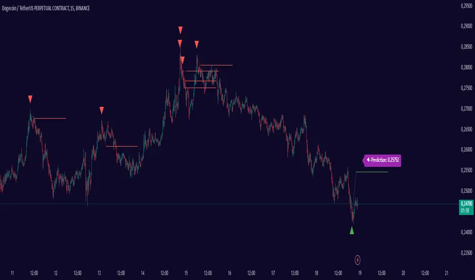
Smart Adaptive Signal SystemSmart Adaptive Signal System
Description: The Smart Adaptive Signal System is a sophisticated indicator that generates intelligent buy/sell signals by dynamically adapting to market conditions. It predicts target prices based on momentum and volatility, providing more accurate and reliable trading opportunities.
How It Works:
Dynamic Signal Generation: The system predicts target prices by considering factors such as volatility and momentum. This allows it to react instantly to trend changes and market fluctuations.
Adaptive Thresholds: Buy and sell signals are triggered with adaptive thresholds, adjusting according to market volatility. This ensures flexibility in the face of sudden market changes.
Trend-Based Reset: Users can choose to reset threshold values based on a time interval or trend change. This feature helps the system re-adapt to current market conditions for greater accuracy.
Target Price Prediction: Target prices are calculated using momentum and volatility, helping the system predict future price movements.
How to Use:
Buy/Sell Signals: The indicator generates buy and sell signals based on market conditions. Look for a "down arrow" for a buy signal and an "up arrow" for a sell signal on the chart.
Target Price Lines: Along with buy and sell signals, the system draws target price lines. This helps you visualize potential future price levels.
Flexible Settings: Users can customize analysis periods, minimum change percentages, and other parameters to fit their needs.
Features:
Dynamic buy and sell signals
Target price predictions
Volatility and momentum-based analysis
User-friendly and flexible settings
Trend-based adaptive resetting
Alerts: The Smart Adaptive Signal System responds quickly to sudden market changes, but always use it in conjunction with other indicators like support and resistance levels. Signal accuracy may vary depending on market conditions.
Flux Charts - SFX Automation💎 GENERAL OVERVIEW
The SFX Automation is a powerful and versatile tool designed to help traders rigorously test their trading strategies against historical market data. With various advanced settings, traders can fine-tune their strategies, assess performance, and identify key improvements before deploying in live trading environments. This tool offers a wide range of configurable settings, explained within this write-up.
Features of the new SFX Automation :
Step By Step : Configure your strategy step by step, which will allow you to have OR & AND logic in your strategies.
Highly Configurable : Offers multiple parameters for fine-tuning trade entry and exit conditions.
Multi-Timeframe Analysis : Allows traders to analyze multiple timeframes simultaneously for enhanced accuracy.
Provides advanced stop-loss, take-profit, and break-even settings.
Incorporates Buy & Sell signals, with settings like Signal Sensitivity, Strength, Time Weighting, Dynamic TP & SL Methods and more for refined strategy execution.
🚩 UNIQUENESS
The SFX Automation stands out from conventional backtesting tools due to its unparalleled flexibility, precision, and advanced trading logic integration. Key factors that make it unique include:
✅ Comprehensive Strategy Customization – Unlike traditional backtesters that offer basic entry and exit conditions, SFX Automation provides a highly detailed parameter set, allowing traders to fine-tune their strategies with precision.
✅ Multi-Timeframe Signals – This is the first-ever tool that allows traders to backtest Buy & Sell Signals on multiple timeframes.
✅ Customizable Take-Profit Conditions – Offers various methods to set take-profit exits, including using core features from SFX Algo, and dynamic exits like signal rating upgrades/downgrades, enabling traders to tailor their exit strategies to specific market behaviors.
✅ Customizable Stop-Loss Conditions – Provides several ways to set up stop losses, including using concepts from SFX Algo and trailing stops or dynamic exits like signal rating upgrades/downgrades, allowing for dynamic risk management tailored to individual strategies.
✅ Integration of External Indicators – Allows the inclusion of other indicators or data sources from TradingView for creating strategy conditions, enabling traders to enhance their strategies with additional insights and data points.
By integrating these advanced features, SFX Automation ensures that traders can rigorously test and optimize their strategies with great accuracy and efficiency.
📌 HOW DOES IT WORK ?
The first setting you will want to set it the pyramiding setting. This setting controls the number of simultaneous trades in the same direction allowed in the strategy. For example, if you set it to 1, only one trade can be active in any time, and the second trade will not be entered unless the first one is exited. If it is set to 2, the script will handle both of them at the same time. Note that you should enter the same value to this pyramiding setting, and the pyramiding setting in the "Properties" tab of the script for this to work.
You can enable and set a backtesting window that will limit the entries to between the start date & end date.
Entry Conditions
From the "Long Conditions" or the "Short Conditions" groups, you can set your position entry conditions. For settings like "initial capital" or "order size", you can open the "Properties" tab, where these are handled.
The SFX Algo can use the following conditions for entry conditions :
1. Buy Signal (Any, or 1-5 ☆)
This condition is triggered when a Buy Signal occurs. Other timeframes are supported with this condition.
2. Buy | TP (1, 2 or 3)
This condition is triggered when a TP signal of any Buy signal occurs.
3. Buy | SL
This condition is triggered when a SL signal of any Buy signal occurs.
4. Buy | Rating Upgrade
This condition is triggered when the rating of a buy signal is increased.
5. Buy | Rating Downgrade
This condition is triggered when the rating of a buy signal is decreased.
6. Sell Signal (Any, or 1-5 ☆)
This condition is triggered when a Sell Signal occurs. Other timeframes are supported with this condition.
7. Sell | TP (1, 2 or 3)
This condition is triggered when a TP signal of any Sell signal occurs.
8. Sell | SL
This condition is triggered when a SL signal of any Sell signal occurs.
9. Sell | Rating Upgrade
This condition is triggered when the rating of a sell signal is increased.
10. Sell | Rating Downgrade
This condition is triggered when the rating of a sell signal is decreased.
11. Retracement Wave Retest (Bullish or Bearish)
A retest on the Retracement Wave occurs when the price temporarily moves against the prevailing trend, touching or entering the wave before continuing in the original trend direction. This retest serves as a confirmation that the wave is acting as dynamic support or resistance.
12. Retracement Wave Retracement (Bullish or Bearish)
A retracement on the Retracement Wave occurs when the price touches the wave, the condition is triggered immediately.
13. Volatility Bands Retest (Bullish or Bearish)
A retest of Volatility Bands occurs when the price initially moves beyond the bands, then pulls back to "retest" the band it just broke through before continuing its move. This can provide traders with confirmation of a breakout or signal a potential reversal.
14. Volatility Bands Retracement (Bullish or Bearish)
A retracement on the Volatility Bands occur when the price touches the band, the condition is triggered immediately.
🕒 TIMEFRAME CONDITIONS
The SFX Automation supports Multi-Timeframe (MTF) features for Buy & Sell signals. When setting an entry condition, you can also choose the timeframe.
External Conditions
Users can use external indicators on the chart to set entry conditions.
The second dropdown in the external condition settings allows you to choose a conditional operator to compare external outputs. Available options include:
Less Than or Equal To: <=
Less Than: <
Equal To: =
Greater Than: >
Greater Than or Equal To: >=
The position entry conditions work like this ;
Each side has 3 SFX Algo conditions and 2 Source conditions. Each condition can be enabled or disabled using the checkbox on the left side of them.
You can select which timeframe this condition should work on for Buy & Sell signals. If you select "Chart", the condition will work for the chart's current timeframe.
Lastly select the step of this condition from 1 to 6.
The Source Condition
The last condition on each side is a source condition that is different from the others. Using this condition, you can create your own logic using other indicators' outputs on your chart. For example, suppose that you have an EMA indicator in your chart. You can have the source condition to something like "EMA > high".
The Step System
Each condition has a step number, and conditions are in topological order based on them.
The conditions are executed step by step. This means the condition with step 2 cannot be executed before the condition with step 1 is executed.
Conditions with the same step numbers have "OR" logic. This means that if you have 2 conditions with step 3, the condition with step 4 can trigger after only one of the step 3 conditions is executed.
➕ OTHER ENTRY FEATURES
The SFX Automation allows traders to choose when to execute trades and when not to execute trades.
1. Only Take Trades
This setting lets users specify the time period when their strategy can open or execute trades.
2. Don't Take Trades
This setting lets users specify time periods when their strategy can't open or execute trades.
↩️ EXIT CONDITIONS
1. Exit on Opposite Signal
When enabled, a long position will close when short entry conditions are met, and a short position will close when long entry conditions are met.
2. Exit on Session End
When enabled, positions will be closed at the end of the trading session.
📈 TAKE PROFIT CONDITIONS
There are several methods available for setting take profit exits and conditions.
1. Entry Condition TP
Users can use entry conditions as triggers for take profit exits. This setting can be found under the long and short exit conditions.
2. Fixed TP
Users can set a fixed TP for exits. This setting can be found under the long and short exit conditions. Users can choose between the following:
Price: This method triggers a TP exit when price reaches a specified level. For example, if you set the Price TP to 10 and buy NASDAQ:TSLA at $190, the trade will automatically exit when the price reaches $200 ($190 + $10).
Ticks: This method triggers a TP exit when price moves a specified number of ticks.
Percentage (%): This method triggers a TP exit when price moves a specified percentage.
ATR: This method triggers a TP exit based on a specified multiple of the Average True Range (ATR).
🧩EXIT PERCENTAGES
For each 3 dynamic take-profit conditions, you can set the amount of the position to exit in terms of percentage. It's important to make sure that the total of the exit percentages are 100%.
📉 STOP LOSS CONDITIONS
There are several methods available for setting stop-loss exits and conditions.
1. Entry Condition SL
Users can use entry conditions as triggers for stop-loss exits. This setting can be found under the long and short exit conditions.
2. Fixed SL
Users can set a fixed SL for exits. This setting can be found under the long and short exit conditions. Users can choose between the following:
Price: This method triggers a SL exit when price reaches a specified level. For example, if you set the Price SL to 10 and buy NASDAQ:TSLA at $200, the trade will automatically exit when the price reaches $190 ($200 - $10).
Ticks: This method triggers a SL exit when price moves a specified number of ticks.
Percentage (%): This method triggers a SL exit when price moves a specified percentage.
ATR: This method triggers a SL exit based on a specified multiple of the Average True Range (ATR).
3. Trailing Stop
An explanation & example for the trailing stop feature is present on the write-up within the next section.
Exit conditions have the same logic of constructing conditions like the entry ones. You can construct a Take-Profit Condition & a Stop-Loss Condition. Note that the Take-Profit condition will only work if the position is in profit, regardless of if it's triggered or not. The same applies for the Stop-Loss condition, meaning that it will only work if the position is in loss.
You can also set a Fixed TP & Fixed SL based on the price movement after the position is entered. You have options like "Price", "Ticks", "%", or "Average True Range". For example, you can set a Fixed TP like "5%", and the position will be entered once it moves 5% up in a long position.
Trailing Stop
For the Fixed SL, you also have a "Trailing" stop option, which you can set it's activation level as well. The Trailing stop activation level and it's value are expressed in ticks. Check this scenerio for an example :
We have a ticker with a tick value of $1. Our Trailing Stop is set to 10 ticks, and the activation level is set to 30 ticks.
We buy 1 contract when the price is $100.
When the price becomes $110, we are in $10 (10 ticks) profit and the trailing stop is now activated.
The current price our stop's on is $110 - $30 (30 ticks), which is the level of $80.
The trailing stop will only move if the price moves up the highest high the price has been after we entered the position.
Let's suppose that price moves up $40 right after our trailing stop is activated. The price will now be $150, and our trailing stop will sit on $150 - $30 (30 ticks) = $120.
If the price is down the $120 level, our stop loss will be triggered.
There is also a "Hard SL" option designed for a backup stop-loss when trailing stops are enabled. You can enable & set this option and if the price goes down before our trailing stop even activates, the position will be exited.
You can also move stop-loss to the break-even (entry price of the position) after a certain profit is achieved using the last setting of the exit conditions. Note that for this to work, you will need to have a Fixed SL setup.
➕ OTHER EXIT FEATURES
1. Move Stop Loss to Breakeven
This setting allows the strategy to automatically move the SL to Breakeven (BE) when the position is in profit by a certain amount. Users can choose between the following:
Price: This method moves the SL to BE when price reaches a specified level.
Ticks: This method moves the SL to BE when price moves a specified number of ticks.
Percentage (%): This method moves the SL to BE when price moves a specified percentage.
ATR: This method moves the SL to BE when price moves a specified multiple of the Average True Range (ATR).
Example Entry Scenario
To give an example , check this scenario; out conditions are :
LONG CONDITIONS
Buy Signal Any☆, Step 1
Bullish R. Wave Retest, Step 2
Bullish V. Bands Retest, Step 2
open > close, Step 3
First, the strategy needs to detect a Buy Signal with any star rating in order to start working.
After it's detected, now it's looking for either a Bullish R. Wave Retest, or a Bullish V. Bands Retest to proceed to the next step, the reason for this is that they both have the same step number.
After one of them is detected, the strategy will consistently check candlesticks for the condition open > close. If a bullish candlestick occurs, a long position will be entered.
⏰ ALERTS
This indicator uses TradingView's strategy alert system. All entries and exits will be sent as an alert if configured. It's possible to further customize these alerts to your liking. For more information, check TradingView's strategy alert customization page: www.tradingview.com
⚙️ SETTINGS
1. Backtesting Settings
Pyramiding: Controls the number of simultaneous trades allowed in the strategy. This setting must have the same value that is entered on the script's properties tab on the settings pane.
Enable Custom Backtesting Period: Restricts backtesting to a specific date range.
Start & End Time Configuration: Define precise start and end dates for historical analysis.
2. Algorithm Settings
Sensitivity: The sensitivity setting is a key parameter that influences the number of signals the SFX Algo generates. By adjusting this parameter, you can control the frequency of signals produced by the algorithm.
Signal Strength: The Signal Strength setting filters signals based on their quality, allowing traders to focus on the most reliable opportunities. This feature helps traders balance the quantity and reliability of the algorithm’s signals to suit their trading strategy.
Time Weighting: The Time Weighting setting determines how the SFX Algo evaluates historical market data to generate signals.
a) Recent Trends
Focuses on the most recent movements for short-term analysis. This setting is good for scalpers and intraday traders who need to react quickly to market changes.
b) Mixed Trends
Balances recent and historical price movements for a comprehensive market view. This setting is well-suited for swing traders and those who want to capture medium-term opportunities by combining the benefits of short-term responsiveness with the reliability of long-term trends.
c) Long-term Trends
Relies on extended historical market data to identify broader market trends, making it an excellent choice for traders focused on long-term strategies.
Minimum Star Rating: The Minimum Star Rating setting allows you to filter signals based on their strength, showing only those that meet or exceed your chosen threshold. For instance, setting the minimum star rating to 3 ensures you only receive signals with a rating of 3 stars or higher.
3. Take Profit / Stop Loss Methods
Key Levels
The Key Levels method uses pivot points to set take profit and stop-loss levels. The TP and SL levels are shown when a new signal is generated.
Volatility Bands
This TP/SL method uses the Volatility Bands overlay to set dynamic TP and SL levels. These levels are not predetermined so they will not be shown in advance when a signal is generated.
Signal Rating
Sets take profit and stop-loss levels based on changes in a signal's rating strength. These levels are not predetermined so they will not be shown in advance when a signal is generated.
Auto Stop-Loss
The auto method can only be applied to the SL. The auto method allows the algorithm to detect SL automatically when a momentum shift is detected. You can adjust the risk tolerance of the Auto SL by adjusting the ‘Auto Risk Tolerance’ setting. You can choose between Low, Medium, and High. A high-risk tolerance will result in stop losses being triggered less often.
4. Entry Conditions for Long & Short Trades
Multiple Conditions (1-6): Configure up to six independent conditions per trade direction.
Timeframe Specification: Choose between timeframes for Buy & Sell signals.
Trade Execution Filters: Restrict trades within specific trading sessions.
5. Exit Conditions for Long & Short Trades
Exit on Opposite Signal: Automatically exit trades upon opposite trade conditions.
Exit on Session End: Closes all positions at the end of the trading session.
Multiple Take-Profit (TP) and Stop-Loss (SL) Configurations:
TP/SL based on % move, ATR, Ticks, or Fixed Price.
Hard SL option for additional risk control.
Move SL to BE (Break Even) after a certain profit threshold.

AI Volume Breakout for scalpingPurpose of the Indicator
This script is designed for trading, specifically for scalping, which involves making numerous trades within a very short time frame to take advantage of small price movements. The indicator looks for volume breakouts, which are moments when trading volume significantly increases, potentially signaling the start of a new price movement.
Key Components:
Parameters:
Volume Threshold (volumeThreshold): Determines how much volume must increase from one bar to the next for it to be considered significant. Set at 4.0, meaning volume must quadruplicate for a breakout signal.
Price Change Threshold (priceChangeThreshold): Defines the minimum price change required for a breakout signal. Here, it's 1.5% of the bar's opening price.
SMA Length (smaLength): The period for the Simple Moving Average, which helps confirm the trend direction. Here, it's set to 20.
Cooldown Period (cooldownPeriod): Prevents signals from being too close together, set to 10 bars.
ATR Period (atrPeriod): The period for calculating Average True Range (ATR), used to measure market volatility.
Volatility Threshold (volatilityThreshold): If ATR divided by the close price exceeds this, the market is considered too volatile for trading according to this strategy.
Calculations:
SMA (Simple Moving Average): Used for trend confirmation. A bullish signal is more likely if the price is above this average.
ATR (Average True Range): Measures market volatility. Lower volatility (below the threshold) is preferred for this strategy.
Signal Generation:
The indicator checks if:
Volume has increased significantly (volumeDelta > 0 and volume / volume >= volumeThreshold).
There's enough price change (math.abs(priceDelta / open) >= priceChangeThreshold).
The market isn't too volatile (lowVolatility).
The trend supports the direction of the price change (trendUp for bullish, trendDown for bearish).
If all these conditions are met, it predicts:
1 (Bullish) if conditions suggest buying.
0 (Bearish) if conditions suggest selling.
Cooldown Mechanism:
After a signal, the script waits for a number of bars (cooldownPeriod) before considering another signal to avoid over-trading.
Visual Feedback:
Labels are placed on the chart:
Green label for bullish breakouts below the low price.
Red label for bearish breakouts above the high price.
How to Use:
Entry Points: Look for the labels on your chart to decide when to enter trades.
Risk Management: Since this is for scalping, ensure each trade has tight stop-losses to manage risk due to the quick, small movements.
Market Conditions: This strategy might work best in markets with consistent volume and price changes but not extreme volatility.
Caveats:
This isn't real AI; it's a heuristic based on volume and price. Actual AI would involve machine learning algorithms trained on historical data.
Always backtest any strategy, and consider how it behaves in different market conditions, not just the ones it was designed for.

Trading IQ - Razor IQIntroducing TradingIQ's first dip buying/shorting all-in-one trading system: Razor IQ.
Razor IQ is an exclusive trading algorithm developed by TradingIQ, designed to trade upside/downside price dips of varying significance in trending markets. By integrating artificial intelligence and IQ Technology, Razor IQ analyzes historical and real-time price data to construct a dynamic trading system adaptable to various asset and timeframe combinations.
Philosophy of Razor IQ
Razor IQ operates on a single premise: Trends must retrace, and these retracements offer traders an opportunity to join in the overarching trend. At some point traders will enter against a trend in aggregate and traders in profitable positions entered during the trend will scale out. When occurring simultaneously, a trend will retrace against itself, offering an opportunity for traders not yet in the trend to join in the move and continue the trend.
Razor IQ is designed to work straight out of the box. In fact, its simplicity requires just a few user settings to manage output, making it incredibly straightforward to manage.
Long Limit Order Stop Loss and Minimum ATR TP/SL are the only settings that manage the performance of Razor IQ!
Traders don’t have to spend hours adjusting settings and trying to find what works best - Razor IQ handles this on its own.
Key Features of Razor IQ
Self-Learning Retracement Detection
Employs AI and IQ Technology to identify notable price dips in real-time.
AI-Generated Trading Signals
Provides retracement trading signals derived from self-learning algorithms.
Comprehensive Trading System
Offers clear entry and exit labels.
Performance Tracking
Records and presents trading performance data, easily accessible for user analysis.
Self-Learning Trading Exits
Razor IQ learns where to exit positions.
Long and Short Trading Capabilities
Supports both long and short positions to trade various market conditions.
How It Works
Razor IQ operates on a straightforward heuristic: go long during the retracement of significant upside price moves and go short during the retracement of significant downside price moves.
IQ Technology, TradingIQ's proprietary AI algorithm, defines what constitutes a “trend” and a “retracement” and what’s considered a tradable dip buying/shorting opportunity. For Razor IQ, this algorithm evaluates all historical trends and retracements, how much trends generally retrace and how long trends generally persist. For instance, the "dip" following an uptrend is measured and learned from, including the significance of the identified trend level (how long it has been active, how much price has increased, etc). By analyzing these patterns, Razor IQ adapts to identify and trade similar future retracements and trends.
In simple terms, Razor IQ clusters previous trend and retracement data in an attempt to trade similar price sequences when they repeat in the future. Using this knowledge, it determines the optimal, current price level where joining in the current trend (during a retracement) has a calculated chance of not stopping out before trend continuation.
For long positions, Razor IQ enters using a market order at the AI-identified long entry price point. If price closes beneath this level a market order will be placed and a long position entered. Of course, this is how the algorithm trades, users can elect to use a stop-limit order amongst other order types for position entry. After the position is entered TP1 is placed (identifiable on the price chart). TP1 has a twofold purpose:
Acts as a legitimate profit target to exit 50% of the position.
Once TP1 is achieved, a stop-loss order is immediately placed at breakeven, and a trailing stop loss controls the remainder of the trade. With this, so long as TP1 is achieved, the position will not endure a loss. So long as price continues to uptrend, Razor IQ will remain in the position.
For short positions, Razor IQ provides an AI-identified short entry level. If price closes above this level a market order will be placed and a short position entered. Again, this is how the algorithm trades, users can elect to use a stop-limit order amongst other order types for position entry. Upon entry Razor IQ implements a TP order and SL order (identifiable on the price chart).
Downtrends, in most markets, usually operate differently than uptrends. With uptrends, price usually increases at a modest pace with consistency over an extended period of time. Downtrends behave in an opposite manner - price decreases rapidly for a much shorter duration.
With this observation, the long dip entry heuristic differs slightly from the short dip entry heuristic.
The long dip entry heuristic specializes in identifying larger, long-term uptrends and entering on retracement of the uptrends. With a dedicated trailing stop loss, so long as the uptrend persists, Razor IQ will remain in the position.
The short dip entry heuristic specializes in identifying sharp, significant downside price moves, and entering short on upside volatility during these moves. A fixed stop loss and profit target are implemented for short positions - no trailing stop is used.
As a trading system, Razor IQ exits all TP orders using a limit order, with all stop losses exited as stop market orders.
What Classifies As a Tradable Dip?
For Razor IQ, tradable price dips are not manually set but are instead learned by the system. What qualifies as an exploitable price dip in one market might not hold the same significance in another. Razor IQ continuously analyzes historical and current trends (if one exists), how far price has moved during the trend, the duration of the trend, the raw-dollar price move of price dips during trends, and more, to determine which future price retracements offer a smart chance to join in any current price trend.
The image above illustrates the Razor Line Long Entry point.
The green line represents the Long Retracement Entry Point.
The blue upper line represents the first profit target for the trade.
The blue lower line represents the trailing stop loss start point for the long position.
The position is entered once price closes below the green line.
The green Razor Lazor long entry point will only appear during uptrends.
The image above shows a long position being entered after the Long Razor Lazor was closed beneath.
Green arrows indicate that the strategy entered a long position at the highlighted price level.
Blue arrows indicate that the strategy exited a position, whether at TP1, the initial stop loss, or at the trailing stop.
Blue lines above the entry price indicate the TP1 level for the current long trade. Blue lines below the current price indicate the initial stop loss price.
If price reaches TP1, a stop loss will be immediately placed at breakeven, and the in-built trailing stop will determine the future exit price.
A blue line (similar to the blue line shown for TP1) will trail price and correspond to the trailing stop price of the trade.
If the trailing stop is above the breakeven stop loss, then the trailing stop will be hit before the breakeven stop loss, which means the remainder of the trade will be exited at a profit.
If the breakeven stop loss is above the trailing stop, then the breakeven stop loss will be hit first. In this case, the remainder of the position will be exited at breakeven.
The image above shows the trailing stop price, represented by a blue line, and the breakeven stop loss price, represented by a pink line, used for the long position!
You can also hover over the trade labels to get more information about the trade—such as the entry price and exit price.
The image above exemplifies Razor IQ's output when a downtrend is active.
When a downtrend is active, Razor IQ will switch to "short mode". In short mode, Razor IQ will display a neon red line. This neon red line indicates the Razor Lazor short entry point. When price closes above the red Razor Lazor line a short position is entered.
The image above shows Razor IQ during an active short position.
The image above shows Razor IQ after completing a short trade.
Red arrows indicate that the strategy entered a short position at the highlighted price level.
Blue arrows indicate that the strategy exited a position, whether at the profit target or the fixed stop loss.
Blue lines indicate the profit target level for the current trade when below price. and blue lines above the current price indicate the stop loss level for the short trade.
Short traders do not utilize a trailing stop - only a fixed profit target and fixed stop loss are used.
You can also hover over the trade labels to get more information about the trade—such as the entry price and exit price.
Minimum Profit Target And Stop Loss
The Minimum ATR Profit Target and Minimum ATR Stop Loss setting control the minimum allowed profit target and stop loss distance. On most timeframes users won’t have to alter these settings; however, on very-low timeframes such as the 1-minute chart, users can increase these values so gross profits exceed commission.
After changing either setting, Razor IQ will retrain on historical data - accounting for the newly defined minimum profit target or stop loss.
AI Direction
The AI Direction setting controls the trade direction Razor IQ is allowed to take.
“Trade Longs” allows for long trades.
“Trade Shorts” allows for short trades.
Verifying Razor IQ’s Effectiveness
Razor IQ automatically tracks its performance and displays the profit factor for the long strategy and the short strategy it uses. This information can be found in the table located in the top-right corner of your chart showing.
This table shows the long strategy profit factor and the short strategy profit factor.
The image above shows the long strategy profit factor and the short strategy profit factor for Razor IQ.
A profit factor greater than 1 indicates a strategy profitably traded historical price data.
A profit factor less than 1 indicates a strategy unprofitably traded historical price data.
A profit factor equal to 1 indicates a strategy did not lose or gain money when trading historical price data.
Using Razor IQ
While Razor IQ is a full-fledged trading system with entries and exits - manual traders can certainly make use of its on chart indications and visualizations.
The hallmark feature of Razor IQ is its ability to signal an acceptable dip entry opportunity - for both uptrends and downtrends. Long entries are often signaled near the bottom of a retracement for an uptrend; short entries are often signaled near the top of a retracement for a downtrend.
Razor IQ will always operate on exact price levels; however, users can certainly take advantage of Razor IQ's trend identification mechanism and retracement identification mechanism to use as confluence with their personally crafted trading strategy.
Of course, every trend will reverse at some point, and a good dip buying/shorting strategy will often trade the reversal in expectation of the prior trend continuing (retracement). It's important not to aggressively filter retracement entries in hopes of avoiding an entry when a trend reversal finally occurs, as this will ultimately filter out good dip buying/shorting opportunities. This is a reality of any dip trading strategy - not just Razor IQ.
Of course, you can set alerts for all Razor IQ entry and exit signals, effectively following along its systematic conquest of price movement.
Paid script

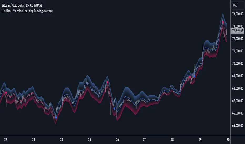
Machine Learning Moving Average [LuxAlgo]The Machine Learning Moving Average (MLMA) is a responsive moving average making use of the weighting function obtained Gaussian Process Regression method. Characteristic such as responsiveness and smoothness can be adjusted by the user from the settings.
The moving average also includes bands, used to highlight possible reversals.
🔶 USAGE
The Machine Learning Moving Average smooths out noisy variations from the price, directly estimating the underlying trend in the price.
A higher "Window" setting will return a longer-term moving average while increasing the "Forecast" setting will affect the responsiveness and smoothness of the moving average, with higher positive values returning a more responsive moving average and negative values returning a smoother but less responsive moving average.
Do note that an excessively high "Forecast" setting will result in overshoots, with the moving average having a poor fit with the price.
The moving average color is determined according to the estimated trend direction based on the bands described below, shifting to blue (default) in an uptrend and fushia (default) in downtrends.
The upper and lower extremities represent the range within which price movements likely fluctuate.
Signals are generated when the price crosses above or below the band extremities, with turning points being highlighted by colored circles on the chart.
🔶 SETTINGS
Window: Calculation period of the moving average. Higher values yield a smoother average, emphasizing long-term trends and filtering out short-term fluctuations.
Forecast: Sets the projection horizon for Gaussian Process Regression. Higher values create a more responsive moving average but will result in more overshoots, potentially worsening the fit with the price. Negative values will result in a smoother moving average.
Sigma: Controls the standard deviation of the Gaussian kernel, influencing weight distribution. Higher Sigma values return a longer-term moving average.
Multiplicative Factor: Adjusts the upper and lower extremity bounds, with higher values widening the bands and lowering the amount of returned turning points.
🔶 RELATED SCRIPTS
Machine-Learning-Gaussian-Process-Regression
SuperTrend-AI-Clustering
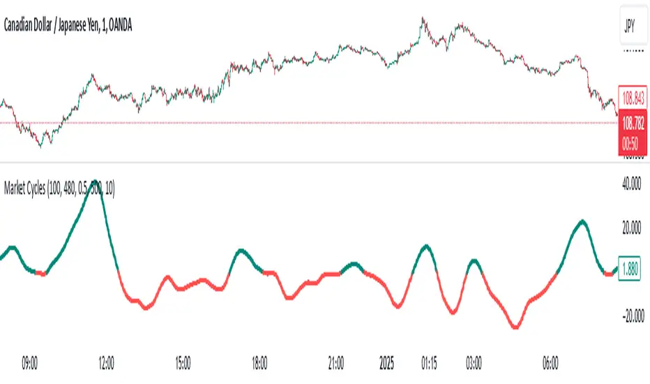
Market Cycles
The Market Cycles indicator transforms market price data into a stochastic wave, offering a unique perspective on market cycles. The wave is bounded between positive and negative values, providing clear visual cues for potential bullish and bearish trends. When the wave turns green, it signals a bullish cycle, while red indicates a bearish cycle.
Designed to show clarity and precision, this tool helps identify market momentum and cyclical behavior in an intuitive way. Ideal for fine-tuning entries or analyzing broader trends, this indicator aims to enhance the decision-making process with simplicity and elegance.
Crypto Index Creator (MEMES & AI Supercycle Dominance, etc)This indicator aims to help to create any INDEX desired including but not limited to its Market Cap and Dominance on the crypto market.
This script was inspired originally by Murad's "Memecoins Dominance" but then I extended it to AI and can be extended to anything in fact, so you can create any index!
I made each token entry editable so that the script can survive the evolution of time as likely projects and INDEXES are going to change a lot, so that you can add/modify your own indices of preference if not listed by default and in order to make it future proof.
You can play with the settings, can compare to BTC, ETC, SOL, etc. for helping in your studies
You also have the option to check the info of each symbol on a table available on the settings, in order to help you figure out if there are any errors and also help you to easily check how the symbols are performing individually
Notes:
- Many projects are not like MEMECOINS that have fixed supply, normally VC projects have a very variable circulating supply, so you might want to update the info of the circulating supply for your projects to make it more accurate if you desire.
- For this script there is a limit of 32 Symbols, due to tradingview own limits, yet you can always "add" multiple projects per line as long as their circulating supply is the same.
- You might want to edit/sort the tickers of the top3, top5 and top10 if they follow bellow those top ranks, but this is not necessary if you don't care about Top 3-10 specific calculations.
- My default "indices" were made of token selections of mine as of November 2024, those defaults indices/tickers I might or might not update them eventually but you are free to adapt/modify the tickers in the settings as history evolves, and you can leave your own indexes on the comment section of this post for others to use
- As you might not be able to create/store multiple different indexes at the same time, you might want to add this indicator multiple times on your screen and then modify the tickers of each instance of this indicator, by that you can have multiple indexes.

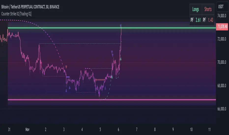
TradingIQ - Counter Strike IQIntroducing "Counter Strike IQ" by TradingIQ
Counter Strike IQ is an exclusive trading algorithm developed by TradingIQ, designed to trade upside/downside breakouts of varying significance. By integrating artificial intelligence and IQ Technology, Counter Strike IQ analyzes historical and real-time price data to construct a dynamic trading system adaptable to various asset and timeframe combinations.
Philosophy of Counter Strike IQ
Counter Strike IQ operates on a single premise: Support and resistance levels cannot hold forever. At some point either side must break for the underlying asset to exhibit trends; otherwise, prices would be confined to an infinitely narrowing range.
Counter Strike IQ is designed to work straight out of the box. In fact, its simplicity requires just four user settings to manage output, making it incredibly straightforward to manage.
Minimum ATR Profit, Minimum ATR Stop, EMA Filter and EMA Filter Length are the only settings that manage the performance of Counter Strike IQ!
Traders don’t have to spend hours adjusting settings and trying to find what works best - Counter Strike IQ handles this on its own.
Key Features of Counter Strike IQ
Self-Learning Breakout Detection
Employs AI and IQ Technology to identify notable breakouts in real-time.
AI-Generated Trading Signals
Provides breakout trading signals derived from self-learning algorithms.
Comprehensive Trading System
Offers clear entry and exit labels.
Performance Tracking
Records and presents trading performance data, easily accessible for user analysis.
Self-Learning Trading Exits
Counter Strike IQ learns where to exit positions.
Long and Short Trading Capabilities
Supports both long and short positions to trade various market conditions.
Strike Channel
The Strike Channel represents what Counter Strike IQ considers a tradable long opportunity or a tradable short opportunity. The Strike Channel is dynamic and adjusts from chart to chart.
IQ Graph Gradient
Introduces the IQ Graph Gradient, designed to classify extreme values in price on a grand scale.
How It Works
Counter Strike IQ operates on a straightforward heuristic: go long during significant upside price moves that break established resistance levels and go short during significant downside price moves that break established support levels.
IQ Technology, TradingIQ's proprietary AI algorithm, defines what constitutes a “significant price move” and what’s considered a tradable breakout. For Counter Strike IQ, this algorithm evaluates all historical support/resistance breaks and any subsequent breakouts. For instance, the price move following up to a breakout is measured and learned from, including the significance of the identified support/resistance level (how long it’s been active, how far price moved away from it, etc). By analyzing these patterns, Counter Strike IQ adapts to identify and trade similar future breakout sequences.
In simple terms, Counter Strike IQ learns from violations of historical support/resistance levels to identify potential entry points at currently established support/resistance levels. Using this knowledge, it determines the optimal, current support/resistance price level where a breakout has a higher chance of occurring.
For long positions, Counter Strike IQ places a stop-market order at the AI-identified resistance point. If price violates this level a market order will be placed and a long position entered. Of course, this is how the algorithm trades, users can elect to use a stop-limit order amongst other order types for position entry. After the position is entered TP1 is placed (identifiable on the price chart). TP1 has a twofold purpose:
Acts as a legitimate profit target to exit 50% of the position.
Once TP1 is closed over, the initial stop loss is converted to a trailing stop, and the long position remains active so long as price continues to uptrend.
For short positions, Counter Strike IQ places a stop-market order at the AI-identified support point. If price violates this level a market order will be placed and a short position entered. Again, this is how the algorithm trades, users can elect to use a stop-limit order amongst other order types for position entry. Upon entry TP1 is placed (identifiable on the price chart). TP1 has a twofold purpose:
Acts as a legitimate profit target to exit 50% of the position.
Once TP1 is closed over, the initial stop loss is converted to a trailing stop, and the short position remains active so long as price continues to downtrend.
As a trading system, Counter Strike IQ exits TP1 using a limit order, with all stop losses exited as stop market orders.
What Classifies As a Tradable Upside Breakout or Tradable Downside Breakout?
For Counter Strike IQ, tradable price breakouts are not manually set but are instead learned by the system. What qualifies as a significant upside or downside breakout in one market might not hold the same significance in another. Counter Strike IQ continuously analyzes historical and current support/resistance levels, how far price has extended from those levels, the raw-dollar price move leading up to a violation of those levels, their longevity, and more, to determine which future levels have a higher chance of breaking out when retested!
The image above illustrates the Strike Channel and explains the corresponding prices and levels
The green upper line represents the Long Breakout Point.
The pink lower line represents the Short Breakout Point.
Any price between the two deviation points is considered “Acceptable”.
The image above shows a long position being entered after the Upside Breakout Point was reached.
Green arrows indicate that the strategy entered a long position at the highlighted price level.
Blue arrows indicate that the strategy exited a position, whether at TP1, the initial stop loss, or at the trailing stop.
Blue lines indicate the TP1 level for the current trade. Red lines indicate the initial stop loss price.
If price closes above TP1, the initial stop loss will be replaced with a trailing stop. A blue line (similar to the blue line shown for TP1) will trail price and correspond to the trailing stop price of the trade.
The image above shows the trailing stop price, represented by a blue line, used for the long position!
You can also hover over the trade labels to get more information about the trade—such as the entry price and exit price.
The image above shows a short position being entered after the Downside Breakout Point was reached.
Red arrows indicate that the strategy entered a short position at the highlighted price level.
Blue arrows indicate that the strategy exited a position, whether at TP1, the initial stop loss, or at the trailing stop.
Blue lines indicate the TP1 level for the current trade. Red lines indicate the initial stop loss price.
If price closes below TP1, the initial stop loss will be replaced with a trailing stop. A blue line (similar to the blue line shown for TP1) will trail price and correspond to the trailing stop price of the trade.
The image above shows the trailing stop price, represented by a blue line, used for the short position!
You can also hover over the trade labels to get more information about the trade—such as the entry price and exit price.
IQ Gradient Graph
The IQ Gradient Graph provides a macro characterization of extreme prices.
The lower macro extremity of the IQ Gradient Graph is colored green, while the upper macro extremity is colored red.
Minimum Profit Target And Stop Loss
The Minimum ATR Profit Target and Minimum ATR Stop Loss setting control the minimum allowed profit target and stop loss distance. On most timeframes users won’t have to alter these settings; however, on very-low timeframes such as the 1-minute chart, users can increase these values so gross profits exceed commission.
After changing either setting, Counter Strike IQ will retrain on historical data - accounting for the newly defined minimum profit target or stop loss.
AI Direction
The AI Direction setting controls the trade direction Counter Strike IQ is allowed to take.
“Trade Longs” allows for long trades.
“Trade Shorts” allows for short trades.
EMA Filter
The EMA Filter setting controls whether the AI should implement an EMA trading filter. Simply, if the EMA Filter is active, long trades can only initiate if price is trading above the user-defined EMA. Conversely, short trades can only initiate if price is trading below the user-defined EMA.
The image above shows the EMA Filter in action!
Verifying Counter Strike IQ’s Effectiveness
Counter Strike IQ automatically tracks its performance and displays the profit factor for the long strategy and the short strategy it uses. This information can be found in the table located in the top-right corner of your chart showing.
This table shows the long strategy profit factor and the short strategy profit factor.
The image above shows the long strategy profit factor and the short strategy profit factor for Counter Strike IQ.
A profit factor greater than 1 indicates a strategy profitably traded historical price data.
A profit factor less than 1 indicates a strategy unprofitably traded historical price data.
A profit factor equal to 1 indicates a strategy did not lose or gain money when trading historical price data.
Using Counter Strike IQ
While Counter Strike IQ is a full-fledged trading system with entries and exits - manual traders can certainly make use of its on chart indications and visualizations.
The hallmark feature of Counter Strike IQ is its ability to signal a breakout near its origin point. Long entries are often signaled near the start of a large upside price move; short entries are often signaled near the start of a large downside price move.
For live analysis, the Strike Channel serves as a valuable tool for identifying breakout points.
The further price moves toward the Upside Breakout Point (green), the stronger the indication that price might breakout to the upside. Conversely, the deeper price reaches toward the Downside Breakout Point (red), the stronger the indication that price might breakout to the downside.
Of course, should buying or selling pressure stall, price may fail to breakout at the identified breakout level. This is a natural consequence of any breakout trading strategy!
With this information at hand, traders can quickly switch between charts and timeframes to identify optimized areas of interest.
Paid script
Machine Learning Signal FilterIntroducing the "Machine Learning Signal Filter," an innovative trading indicator designed to leverage the power of machine learning to enhance trading strategies. This tool combines advanced data processing capabilities with user-friendly customization options, offering traders a sophisticated yet accessible means to optimize their market analysis and decision-making processes. Importantly, this indicator does not repaint, ensuring that signals remain consistent and reliable after they are generated.
Machine Learning Integration
The "Machine Learning Signal Filter" employs machine learning algorithms to analyze historical price data and identify patterns that may not be immediately apparent through traditional technical analysis. By utilizing techniques such as regression analysis and neural networks, the indicator continuously learns from new data, refining its predictive capabilities over time. This dynamic adaptability allows the indicator to adjust to changing market conditions, potentially improving the accuracy of trading signals.
Key Features and Benefits
Dynamic Signal Generation: The indicator uses machine learning to generate buy and sell signals based on complex data patterns. This approach enables it to adapt to evolving market trends, offering traders timely and relevant insights. Crucially, the indicator does not repaint, providing reliable signals that traders can trust.
Customizable Parameters: Users can fine-tune the indicator to suit their specific trading styles by adjusting settings such as the temporal synchronization and neural pulse rate. This flexibility ensures that the indicator can be tailored to different market environments.
Visual Clarity and Usability: The indicator provides clear visual cues on the chart, including color-coded signals and optional display of signal curves. Users can also customize the table's position and text size, enhancing readability and ease of use.
Comprehensive Performance Metrics: The indicator includes a detailed metrics table that displays key performance indicators such as return rates, trade counts, and win/loss ratios. This feature helps traders assess the effectiveness of their strategies and make data-driven decisions.
How It Works
The core of the "Machine Learning Signal Filter" is its ability to process and learn from large datasets. By applying machine learning models, the indicator identifies potential trading opportunities based on historical data patterns. It uses regression techniques to predict future price movements and neural networks to enhance pattern recognition. As new data is introduced, the indicator refines its algorithms, improving its accuracy and reliability over time.
Use Cases
Trend Following: Ideal for traders seeking to capitalize on market trends, the indicator helps identify the direction and strength of price movements.
Scalping: With its ability to provide quick signals, the indicator is suitable for scalpers aiming for rapid profits in volatile markets.
Risk Management: By offering insights into trade performance, the indicator aids in managing risk and optimizing trade setups.
In summary, the "Machine Learning Signal Filter" is a powerful tool that combines the analytical strength of machine learning with the practical needs of traders. Its ability to adapt and provide actionable insights makes it an invaluable asset for navigating the complexities of financial markets.
The "Machine Learning Signal Filter" is a tool designed to assist traders by providing insights based on historical data and machine learning techniques. It does not guarantee profitable trades and should be used as part of a comprehensive trading strategy. Users are encouraged to conduct their own research and consider their financial situation before making trading decisions. Trading involves significant risk, and it is possible to lose more than the initial investment. Always trade responsibly and be aware of the risks involved.

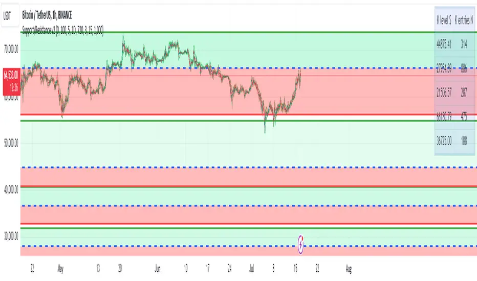
Support/Resistance v2 (ML) KmeanKmean with Standard Deviation Channel
1. Description of Kmean
Kmean (or K-means) is a popular clustering algorithm used to divide data into K groups based on their similarity. In the context of financial markets, Kmean can be applied to find the average price values over a specific period, allowing the identification of major trends and levels of support and resistance.
2. Application in Trading
In trading, Kmean is used to smooth out the price series and determine long-term trends. This helps traders make more informed decisions by avoiding noise and short-term fluctuations. Kmean can serve as a baseline around which other analytical tools, such as channels and bands, are constructed.
3. Description of Standard Deviation (stdev)
Standard deviation (stdev) is a statistical measure that indicates how much the values of data deviate from their mean value. In finance, standard deviation is often used to assess price volatility. A high standard deviation indicates strong price fluctuations, while a low standard deviation indicates stable movements.
4. Combining Kmean and Standard Deviation to Predict Short-Term Price Behavior
Combining Kmean and standard deviation creates a powerful tool for analyzing market conditions. Kmean shows the average price trend, while the standard deviation channels demonstrate the boundaries within which the price can fluctuate. This combination helps traders to:
Identify support and resistance levels.
Predict potential price reversals.
Assess risks and set stop-losses and take-profits.
Should you have any questions about code, please reach me at Tradingview directly.
Hope you find this script helpful!
Edge AI Forecast [Edge Terminal]This indicator inputs the previous 150 closing prices in a simple two-layer neural network, normalizes the network inputs using a sigmoid function, uses a feedforward calculation to send it to the second layer, shows the MSE loss curve and uses both automatic and manual backpropagation (user input) to find the most likely forecast values and uses the analog forecasting algorithm to adjust and optimize the data furthermore to display potential prices on the chart.
Here's how it works:
The idea behind this script is to train a simple neural network to predict the future x values based on the sample data. For this, we use 2 types of data, Price and Volume.
The thinking behind this is that price alone can’t be used in this case because it doesn’t provide enough meaningful pattern data for the network but price and volume together can change the game. We’re planning to use more different data sets and expand on this in the future.
To avoid a bad mix of results, we technically have two neural networks, each processing a different data type, one for volume data and one for price data.
The actual prediction is decided by the way price and volume of the closing price relate to each other. Basically, the network passes the price and volume and finds the best relation between the two data set outputs and predicts where the price could be based on the upcoming volume of the latest candle.
The network adjusts the weights and biases using optimization algorithms like gradient descent to minimize the difference between the predicted and actual stock prices, typically measured by a loss function, (in this case, mean squared error) which you can see using the error rate bubble.
This is a good measure to see how well the network is performing and the idea is to adjust the settings inputs such as learning rate, epochs and data source to get the lowest possible error rate. That’s when you’re getting the most accurate prediction results.
For each data set, we use a multi-layer network. In a multi-layer neural network, the outputs of neurons in one layer serve as inputs to neurons in the next layer. Initially, the input layer of the neural network receives the historical data. Each input neuron represents a feature, such as previous stock prices and trading volumes over a specific period.
The hidden layers perform feature extraction and transformation through a series of weighted connections and activation functions. Each neuron in a hidden layer computes a weighted sum of the inputs from the previous layer, applies an activation function to the sum, and passes the result to the next layer using the feedforward (activation) function.
For extraction, we use a normalization function. This function takes a value or data (such as bar price) and divides it up by max scale which is the highest possible value of the bar. The idea is to take a normalized number, which is either below 1 or under 2 for simple use in the neural network layers.
For the activation, after computing the weighted sum, the neuron applies an activation function a(x). To introduce non-linearity into the model to pass it to the next layer. We use sigmoid activation functions in this case. The main reason we use sigmoid function is because the resulting number is between 0 to 1 and is better for models where we have to predict the probability as an output.
The final output of the network is passed as an input to the analog forecasting function. This is an algorithm commonly used in weather prediction systems. In this case, this is used to make predictions by comparing current values and assuming the patterns might repeat in the future.
There are many different ways to build an analog forecasting function but in our case, we’re used similarity measurement model:
X, as the current situation or set of current variables.
Y, as the outcome or variable of interest.
Si as the historical situations or patterns, where i ranges from 1 to n.
Vi as the vector of variables describing historical situation Si.
Oi as the outcome associated with historical situation Si.
First, we define a similarity measure sim(X,Vi) that quantifies the similarity between the current situation X and historical situation Si based on their respective variables Vi.
Then we select the K most similar historical situations (KNN Machine learning) based on the similarity measure sim(X,Vi). We denote the rest of the selected historical situations as {Si1, Si2,...Sik).
Then we examine the outcomes associated with the selected historical situations {Oi1, Oi2,...,Oik}.
Then we use the outcomes of the selected historical situations to forecast the future outcome Y^ using weighted averaging.
Finally, the output value of the analog forecasting is standardized using a standardization function which is the opposite of the normalization function. This function takes a normalized number and turns it back to its original value by multiplying it by the max scale (highest value of the bar). This function is used when the final number is produced by the network output at the end of the analog forecasting to turn the final value back into a price so it can be displayed on the chart with PineScript.
Settings:
Data source: Source of the neural network's input data.
Sample Bars: How many historical bars do you want to input into the neural network
Prediction Bars: How many bars you want the script to forecast
Show Training Rate: This shows the neural network's error rate for the optimization phase
Learning Rate: how many times you want the script to change the model in response to the estimated error (automatic)
Epochs: the network cycle or how many times you want to run the data through the network from the first layer to the last one.
Usage:
The sample bars input determines the number of historical bars to be used as a reference for the network. You need to change the Epochs and Learning Rate inputs for each asset and chart timeframe to get the lowest error rate.
On the surface, the highest possible epoch and learning rate should produce the most effective results but that's not always the case.
If the epochs rate is too high, there is a chance we face overfitting. Essentially, you might be over processing good data which can make it useless.
On the other hand, if the learning rate is too high, the network may overshoot the optimal solution and diverge. This is almost like the same issue I mentioned above with a high epoch rate.
Access:
It took over 4 months to develop this script and we’re constantly improving it so it took a lot of manpower to develop this script. Also when it comes to neural networks, Pine Script isn’t the most optimal language to build a neural network in, so we had to resort to a few proprietary mathematical formulas to ensure this runs smoothly without giving out an error for overprocessing, specially when you have multiple neural networks with many layers.
The optimization done to make this script run on Pine Script is basically state of the art and because of this, we would like to keep the code closed source at the moment.
On the other hand we don’t want to publish the code publicly as we want to keep the trading edge this script gives us in a closed loop, for our own small group of members so we have to keep the code closed. We only accept invites from expert traders who understand how this script and algo trading works and the type of edge it provides.
Additionally, at the moment we don’t want to share the code as some of the parts of this network, specifically the way we hand the data from neural network output into the analog method formula are proprietary code and we’d like to keep it that way.
You can contact us for access and if we believe this works for your trading case, we will provide you with access.
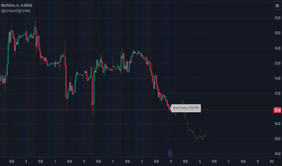
MBAND 200 4H BTC/USDT - By MGS-TradingMBAND 200 4H BTC/USDT with RSI and Volume by MGS-Trading: A Neural Network-Inspired Indicator
Introduction:
The MBAND 200 4H BTC/USDT with RSI and Volume represents a groundbreaking achievement in the integration of artificial intelligence (AI) into cryptocurrency market analysis. Developed by MGS-Trading, this indicator is the culmination of extensive research and development efforts aimed at leveraging AI's power to enhance trading strategies. By synthesizing neural network concepts with traditional technical analysis, the MBAND indicator offers a dynamic, multi-dimensional view of the market, providing traders with unparalleled insights and actionable signals.
Innovative Approach:
Our journey to create the MBAND indicator began with a simple question: How can we mimic the decision-making prowess of a neural network in a trading indicator? The answer lay in the weighted aggregation of Exponential Moving Averages (EMAs) from multiple timeframes, each serving as a unique input akin to a neuron in a neural network. These weights are not arbitrary; they were painstakingly optimized through backtesting across various market conditions to ensure they reflect the significance of each timeframe’s contribution to overall market dynamics.
Core Features:
Neural Network-Inspired Weights: The heart of the MBAND indicator lies in its AI-inspired weighting system, which treats each timeframe’s EMA as an input node in a neural network. This allows the indicator to process complex market data in a nuanced and sophisticated manner, leading to more refined and informed trading signals.
Multi-Timeframe EMA Analysis: By analyzing EMAs from 15 minutes to 3 days, the MBAND indicator captures a comprehensive snapshot of market trends, enabling traders to make informed decisions based on a broad spectrum of data.
RSI and Volume Integration: The inclusion of the Relative Strength Index (RSI) and volume data adds layers of confirmation to the signals generated by the EMA bands. This multi-indicator approach helps in identifying high-probability setups, reinforcing the neural network’s concept of leveraging multiple data points for decision-making.
Usage Guidelines:
Signal Interpretation: The MBAND bands provide a visual representation of the market’s momentum and direction. A price moving above the upper band signals strength and potential continuation of an uptrend, while a move below the lower band suggests weakness and a possible downtrend.
Overbought/Oversold Conditions: The RSI component identifies when the asset is potentially overbought (>70) or oversold (<30). Traders should watch for these conditions near the MBAND levels for potential reversal opportunities.
Volume Confirmation: An increase in volume accompanying a price move towards or beyond an MBAND level serves as confirmation of the strength behind the move. This can indicate whether a breakout is likely to sustain or if a reversal has substantial backing.
Strategic Entry and Exit Points: Combine the MBAND readings with RSI and volume indicators to pinpoint strategic entry and exit points. For example, consider entering a long position when the price is near the lower MBAND, RSI indicates oversold conditions, and there is a notable volume increase.
About MGS-Trading:
At MGS-Trading, we are passionate about harnessing the transformative power of AI to revolutionize cryptocurrency trading. Our indicators and tools are designed to provide traders with advanced analytics and insights, drawing on the latest AI techniques and methodologies. The MBAND 200 4H BTC/USDT with RSI and Volume indicator is a prime example of our commitment to innovation, offering traders a sophisticated, AI-enhanced tool for navigating the complexities of the cryptocurrency markets.
Disclaimer:
The MBAND indicator is provided for informational purposes only and does not constitute investment advice. Trading cryptocurrencies involves significant risk and can result in the loss of your investment. We recommend conducting your own research and consulting with a qualified financial advisor before making any trading decisions.

AI Adaptive Money Flow Index (Clustering) [AlgoAlpha]🌟🚀 Dive into the future of trading with our latest innovation: the AI Adaptive Money Flow Index by AlgoAlpha Indicator! 🚀🌟
Developed with the cutting-edge power of Machine Learning, this indicator is designed to revolutionize the way you view market dynamics. 🤖💹 With its unique blend of traditional Money Flow Index (MFI) analysis and advanced k-means clustering, it adapts to market conditions like never before.
Key Features:
📊 Adaptive MFI Analysis: Utilizes the classic MFI formula with a twist, adjusting its parameters based on AI-driven clustering.
🧠 AI-Driven Clustering: Applies k-means clustering to identify and adapt to market states, optimizing the MFI for current conditions.
🎨 Customizable Appearance: Offers adjustable settings for overbought, neutral, and oversold levels, as well as colors for uptrends and downtrends.
🔔 Alerts for Key Market Movements: Set alerts for trend reversals, overbought, and oversold conditions, ensuring you never miss a trading opportunity.
Quick Guide to Using the AI Adaptive MFI (Clustering):
🛠 Customize the Indicator: Customize settings like MFI source, length, and k-means clustering parameters to suit your analysis.
📈 Market Analysis: Monitor the dynamically adjusted overbought, neutral, and oversold levels for insights into market conditions. Watch for classification symbols ("+", "0", "-") for immediate understanding of the current market state. Look out for reversal signals (▲, ▼) to get potential entry points.
🔔 Set Alerts: Utilize the built-in alert conditions for trend changes, overbought, and oversold signals to stay ahead, even when you're not actively monitoring the charts.
How It Works:
The AI Adaptive Money Flow Index employs the k-means clustering machine learning algorithm to refine the traditional Money Flow Index, dynamically adjusting overbought, neutral, and oversold levels based on market conditions. This method analyzes historical MFI values, grouping them into initial clusters using the traditional MFI's overbought, oversold and neutral levels, and then finding the mean of each cluster, which represent the new market states thresholds. This adaptive approach ensures the indicator's sensitivity in real-time, offering a nuanced understanding of market trend and volume analysis.
By recalibrating MFI thresholds for each new data bar, the AI Adaptive MFI intelligently conforms to changing market dynamics. This process, assessing past periods to adjust the indicator's parameters, provides traders with insights finely tuned to recent market behavior. Such innovation enhances decision-making, leveraging the latest data to inform trading strategies. 🌐💥
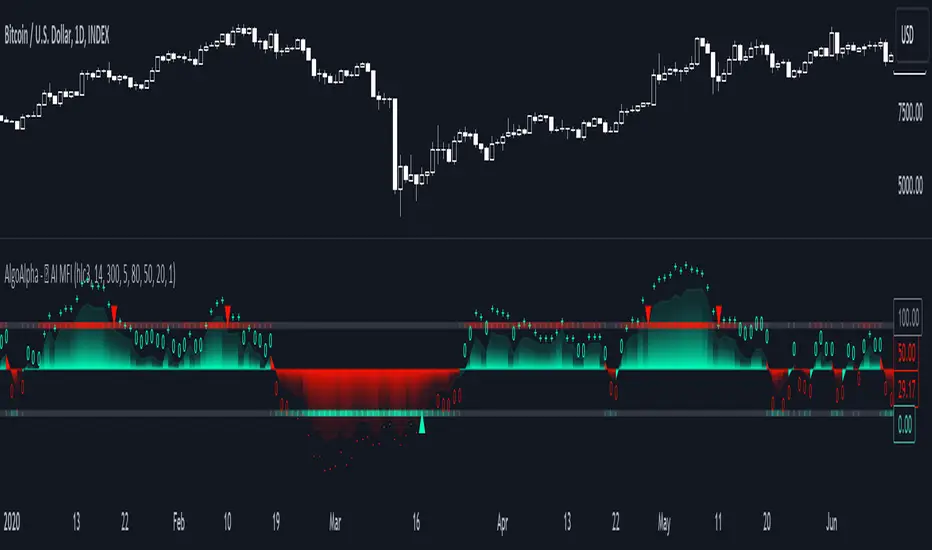
Machine Learning: Multiple Logistic Regression
Multiple Logistic Regression Indicator
The Logistic Regression Indicator for TradingView is a versatile tool that employs multiple logistic regression based on various technical indicators to generate potential buy and sell signals. By utilizing key indicators such as RSI, CCI, DMI, Aroon, EMA, and SuperTrend, the indicator aims to provide a systematic approach to decision-making in financial markets.
How It Works:
Technical Indicators:
The script uses multiple technical indicators such as RSI, CCI, DMI, Aroon, EMA, and SuperTrend as input variables for the logistic regression model.
These indicators are normalized to create categorical variables, providing a consistent scale for the model.
Logistic Regression:
The logistic regression function is applied to the normalized input variables (x1 to x6) with user-defined coefficients (b0 to b6).
The logistic regression model predicts the probability of a binary outcome, with values closer to 1 indicating a bullish signal and values closer to 0 indicating a bearish signal.
Loss Function (Cross-Entropy Loss):
The cross-entropy loss function is calculated to quantify the difference between the predicted probability and the actual outcome.
The goal is to minimize this loss, which essentially measures the model's accuracy.
// Error Function (cross-entropy loss)
loss(y, p) =>
-y * math.log(p) - (1 - y) * math.log(1 - p)
// y - depended variable
// p - multiple logistic regression
Gradient Descent:
Gradient descent is an optimization algorithm used to minimize the loss function by adjusting the weights of the logistic regression model.
The script iteratively updates the weights (b1 to b6) based on the negative gradient of the loss function with respect to each weight.
// Adjusting model weights using gradient descent
b1 -= lr * (p + loss) * x1
b2 -= lr * (p + loss) * x2
b3 -= lr * (p + loss) * x3
b4 -= lr * (p + loss) * x4
b5 -= lr * (p + loss) * x5
b6 -= lr * (p + loss) * x6
// lr - learning rate or step of learning
// p - multiple logistic regression
// x_n - variables
Learning Rate:
The learning rate (lr) determines the step size in the weight adjustment process. It prevents the algorithm from overshooting the minimum of the loss function.
Users can set the learning rate to control the speed and stability of the optimization process.
Visualization:
The script visualizes the output of the logistic regression model by coloring the SMA.
Arrows are plotted at crossover and crossunder points, indicating potential buy and sell signals.
Lables are showing logistic regression values from 1 to 0 above and below bars
Table Display:
A table is displayed on the chart, providing real-time information about the input variables, their values, and the learned coefficients.
This allows traders to monitor the model's interpretation of the technical indicators and observe how the coefficients change over time.
How to Use:
Parameter Adjustment:
Users can adjust the length of technical indicators (rsi_length, cci_length, etc.) and the Z score length based on their preference and market characteristics.
Set the initial values for the regression coefficients (b0 to b6) and the learning rate (lr) according to your trading strategy.
Signal Interpretation:
Buy signals are indicated by an upward arrow (▲), and sell signals are indicated by a downward arrow (▼).
The color-coded SMA provides a visual representation of the logistic regression output by color.
Table Information:
Monitor the table for real-time information on the input variables, their values, and the learned coefficients.
Keep an eye on the learning rate to ensure a balance between model adjustment speed and stability.
Backtesting and Validation:
Before using the script in live trading, conduct thorough backtesting to evaluate its performance under different market conditions.
Validate the model against historical data to ensure its reliability.
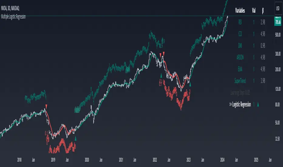
Machine Learning: STDEV Oscillator [YinYangAlgorithms]This Indicator aims to fill a gap within traditional Standard Deviation Analysis. Rather than its usual applications, this Indicator focuses on applying Standard Deviation within an Oscillator and likewise applying a Machine Learning approach to it. By doing so, we may hope to achieve an Adaptive Oscillator which can help display when the price is deviating from its standard movement. This Indicator may help display both when the price is Overbought or Underbought, and likewise, where the price may face Support and Resistance. The reason for this is that rather than simply plotting a Machine Learning Standard Deviation (STDEV), we instead create a High and a Low variant of STDEV, and then use its Highest and Lowest values calculated within another Deviation to create Deviation Zones. These zones may help to display these Support and Resistance locations; and likewise may help to show if the price is Overbought or Oversold based on its placement within these zones. This Oscillator may also help display Momentum when the High and/or Low STDEV crosses the midline (0). Lastly, this Oscillator may also be useful for seeing the spacing between the High and Low of the STDEV; large spacing may represent volatility within the STDEV which may be helpful for seeing when there is Momentum in the form of volatility.
Tutorial:
Above is an example of how this Indicator looks on BTC/USDT 1 Day. As you may see, when the price has parabolic movement, so does the STDEV. This is due to this price movement deviating from the mean of the data. Therefore when these parabolic movements occur, we create the Deviation Zones accordingly, in hopes that it may help to project future Support and Resistance locations as well as helping to display when the price is Overbought and Oversold.
If we zoom in a little bit, you may notice that the Support Zone (Blue) is smaller than the Resistance Zone (Orange). This is simply because during the last Bull Market there was more parabolic price deviation than there was during the Bear Market. You may see this if you refer to their values; the Resistance Zone goes to ~18k whereas the Support Zone is ~10.5k. This is completely normal and the way it is supposed to work. Due to the nature of how STDEV works, this Oscillator doesn’t use a 1:1 ratio and instead can develop and expand as exponential price action occurs.
The Neutral (0) line may also act as a Support and Resistance location. In the example above we can see how when the STDEV is below it, it acts as Resistance; and when it’s above it, it acts as Support.
This Neutral line may also provide us with insight as towards the momentum within the market and when it has shifted. When the STDEV is below the Neutral line, the market may be considered Bearish. When the STDEV is above the Neutral line, the market may be considered Bullish.
The Red Line represents the STDEV’s High and the Green Line represents the STDEV’s Low. When the STDEV’s High and Low get tight and close together, this may represent there is currently Low Volatility in the market. Low Volatility may cause consolidation to occur, however it also leaves room for expansion.
However, when the STDEV’s High and Low are quite spaced apart, this may represent High levels of Volatility in the market. This may mean the market is more prone to parabolic movements and expansion.
We will conclude our Tutorial here. Hopefully this has given you some insight into how applying Machine Learning to a High and Low STDEV then creating Deviation Zones based on it may help project when the Momentum of the Market is Bullish or Bearish; likewise when the price is Overbought or Oversold; and lastly where the price may face Support and Resistance in the form of STDEV.
If you have any questions, comments, ideas or concerns please don't hesitate to contact us.
HAPPY TRADING!
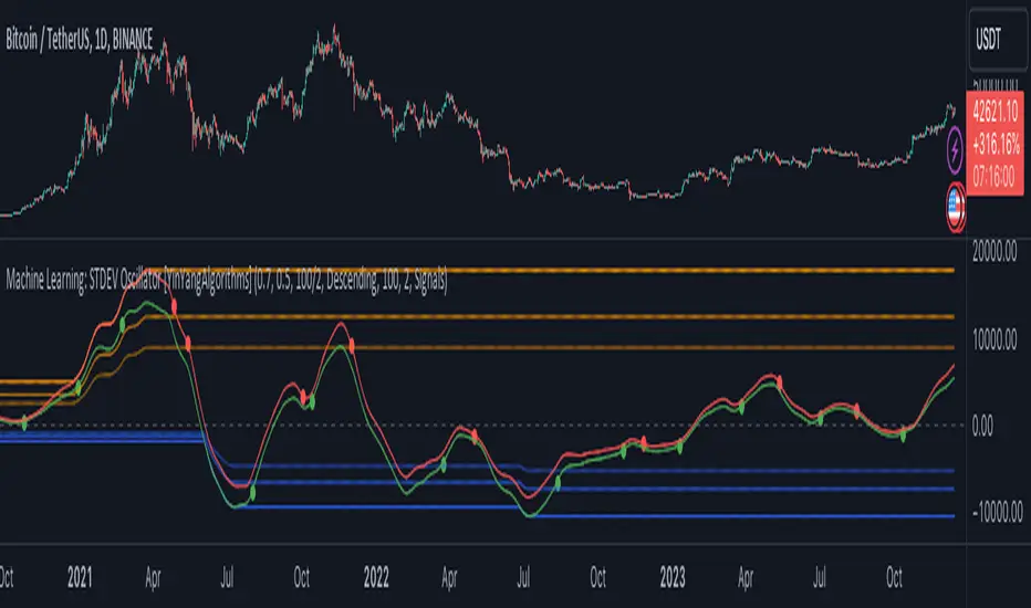
Machine Learning: Optimal Length [YinYangAlgorithms]This Indicator aims to solve an issue that most others face; static lengths. This Indicator will scan lengths from the Min to Max setting (1 - 400 by default) to calculate which is the most Optimal Length in the current market condition. Almost every Indicator uses a length in some part of their calculation, and this length is usually adjustable via the Settings; however it is generally a static fixed length. Static non changing lengths may not always produce optimal results. As market conditions change generally the optimal length will too. For this reason we have created this indicator.
This Indicator will create a Neutral (Min - Max Length), Fast (Min - Mid Length ((Max - Min) / 2)) and Slow (Mid Length ((Max - Min) / 2) - Max Length). This allows you to understand which the Optimal Fast, Slow and Neutral lengths are within the given Mix and Max length settings.
This Indicator then plots these Optimal Lengths as an Oscillator which can then be used within ANOTHER Indicator as a Source within its Settings. Stand alone this Indicator may not prove all that useful, however when its Lengths are inputted into another Indicator it may prove very useful. This allows other Indicators to use the Optimal Length within its calculations from the Settings rather than relying on simply a fixed length. Unfortunately this results in users needing to manually plug the Optimal Length plots into the second Indicator; but it also allows for endless possibilities with applying Machine Learning Optimal Lengths within both Traditional and Non-Traditional Indicators and may give other Pine Coders an easy and effective way to add Machine Learning auto adjustable lengths within their already created Indicators.
The beautiful part about this Indicator is that aside from inputting the Optimal Length Plot into another Indicator, there is no manual updating needed. When the Optimal Length changes, the change will automatically reflect in the other Indicator without the need for you to manually adjust its length. This may be very useful with both time preservation, as well as if there is an automated strategy based upon said Indicator that now won’t need manual intervention.
Tutorial:
By default this is what the Machine Learning: Optimal Length Indicator looks like. It is simply a way of both Displaying and Plotting our current Optimal Length so that we may then use it as a source within ANOTHER Indicator. This will allow the automation of an Optimal Length to be updated, rather than needing any manual input from yourself (aside from set up).
For instance if you set the start length to 1 and the end length to 400 (default settings), it will scan to find the optimal Length setting between 1 and 400. This features 3 types of lengths:
Fast (Green Line): 1-199 (from start length to half way of total)
Slow (Red Line): 200 - 400 (mid way to end length)
Neutral (Blue Line): 1 - 400 (start to end length)
By breaking down the Optimal Length detection into these 3 different types, we can see how the Optimal Length compares and changes based on the lengths allotted to them and how performance changes.
For instance, you may notice that both the Fast and Slow Optimal Length didn’t change much in the example above; however the Neutral Optimal Length changed quite a bit. This is due to the fact that the Neutral is inclusive of all lengths available and may be considered the more accurate due to that. However, this doesn’t mean the Fast and Slow lengths aren’t important and should be used. They may be useful for seeing how something fairs in a Fast and Slow standpoint.
If you change your TimeFrame from 15 minute to 1 Day, you’ll notice that the Optimal Lengths gravitate towards their upper bounds:
199 is max for Fast, it’s at 195
400 is max for Slow, its at 393
400 is max for Neutral, its at 399
The Optimal Length may move up to its upper bounds on Higher Time Frames because there is a lot of price action and long term data being displayed. This may lead to higher lengths performing better in a profitability standpoint since its data is based on so far back and such drastic price movements.
Below we’re going to go through a few examples, including the code so you may reproduce the example and have an understanding of how versatile Inputting an Optimal Length as a source may be within Traditional Indicators.
Adding the Machine Learning: Optimal Length to another Indicator:
You may add the Optimal Length to another Indicator as shown in the example above. In the example we are adding the ‘Machine Learning: Optimal Length - Neutral’ to our Neutral Length within the Settings. The external Indicator needs to have the ability to input the Optimal Length as a Source, this way it can automatically change within the external Indicator when the Optimal Length Indicator changes its Optimal Length.
Please note you may get an error within an external Indicator that accepts the Length as a Source if you don’t select the Machine Learning: Optimal Length. For instance, if you use ‘Close’ within BTC/USDT the length used would be ~36,000. This length is too long and will throw an error.
For this reason, we will ensure the Max Length that may be used is 1000.
Please note, on lower Time Frames you may need to adjust the Max Length. For instance if 20k bar data is used, the Max Length ‘may’ fail to load when going by default Min: 1 and Max: 400. Generally with most pairs it will load if your TradingView subscription is Premium or greater; however if it is less there is a chance it may fail. If it fails for you too often please lower the Max Length Amount; or send us a message we can look into a fix for this.
*** If it fails to load, please try removing the external Indicator and re-adding it and adding the Lengths back as a Source within the Settings. Sometimes it fails, but re-adding may fix it. If it keeps failing afterwards, reduce the Max Length Amount as mentioned above. ***
Simple Moving Average:
In this example above have the Fast, Slow and Neutral Optimal Length formatted as a Slow Moving Average. The first example is on the 15 minute Time Frame and the second is on the 1 Day Time Frame, demonstrating how the length changes based on the Time Frame and the effects it may have.
Here is the code for the example Indicator shown above. This example shows how you may use the Optimal Length as a Source and then use that Optimal Length and plot it as a Simple Moving Average:
//@version=5
indicator("Optimal Length - Backtesting - MA", overlay=true, max_bars_back=5000)
outputType = input.string("All", "Output Type", options= )
lengthSource = input.source(close, "Neutral Length")
lengthSource_fast = input.source(close, "Fast Length")
lengthSource_slow = input.source(close, "Slow Length")
showNeutral = outputType == "Neutral" or outputType == "Fast + Neutral" or outputType == "Slow + Neutral" or outputType == "All"
showFast = outputType == "Fast" or outputType == "Fast + Neutral" or outputType == "Fast + Slow" or outputType == "All"
showSlow = outputType == "Slow" or outputType == "Slow + Neutral" or outputType == "Fast + Slow" or outputType == "All"
//Neutral
optimalLength = math.min(math.max(math.round(lengthSource), 1), 1000)
optimalMA = ta.sma(close, optimalLength)
//Fast
optimalLength_fast = math.min(math.max(math.round(lengthSource_fast), 1), 1000)
optimalMA_fast = ta.sma(close, optimalLength_fast)
//Slow
optimalLength_slow = math.min(math.max(math.round(lengthSource_slow), 1), 1000)
optimalMA_slow = ta.sma(close, optimalLength_slow)
plot(showNeutral ? optimalMA : na, color=color.blue)
plot(showFast ? optimalMA_fast : na, color=color.green)
plot(showSlow ? optimalMA_slow : na, color=color.red)
Bollinger Bands:
In the two examples above for Bollinger Bands we have first the 15 Minute Time Frame and then the 1 Day Time Frame. As described above in ‘Adding the Machine Learning: Optimal Length to another Indicator’ sometimes it may fail to load, for this reason in the 15 Minute it was reduced to a max of 300 Length.
Bollinger Bands are a way to see a Simple Moving Average (SMA) that then uses Standard Deviation to identify how much deviation has occurred. This Deviation is than Added and Subtracted from the SMA to create the Bollinger Bands which help Identify possible movement zones that are ‘within range’. This may mean that the price may face Support / Resistance when it reaches the Outer / Inner bounds of the Bollinger Bands. Likewise, it may mean the Price is ‘Overbought’ when outside and above or ‘Underbought’ when outside and below the Bollinger Bands.
By applying All 3 different types of Optimal Lengths towards a Traditional Bollinger Band calculation we may hope to see different ranges of Bollinger Bands and how different lookback lengths may imply possible movement ranges on both a Short Term, Long Term and Neutral perspective. By seeing these possible ranges you may have the ability to identify more levels of Support and Resistance over different lengths and Trading Styles.
Below is the code for the Bollinger Bands example above:
//@version=5
indicator("Optimal Length - Backtesting - Bollinger Bands", overlay=true, max_bars_back=5000)
outputType = input.string("All", "Output Type", options= )
lengthSource = input.source(close, "Neutral Length")
lengthSource_fast = input.source(close, "Fast Length")
lengthSource_slow = input.source(close, "Slow Length")
showNeutral = outputType == "Neutral" or outputType == "Fast + Neutral" or outputType == "Slow + Neutral" or outputType == "All"
showFast = outputType == "Fast" or outputType == "Fast + Neutral" or outputType == "Fast + Slow" or outputType == "All"
showSlow = outputType == "Slow" or outputType == "Slow + Neutral" or outputType == "Fast + Slow" or outputType == "All"
mult = 2.0
src = close
neutralColor = color.blue
slowColor = color.red
fastColor = color.green
//Neutral
optimalLength = math.min(math.max(math.round(lengthSource), 1), 1000)
optimalMA = ta.sma(close, optimalLength)
//Fast
optimalLength_fast = math.min(math.max(math.round(lengthSource_fast), 1), 1000)
optimalMA_fast = ta.sma(close, optimalLength_fast)
//Slow
optimalLength_slow = math.min(math.max(math.round(lengthSource_slow), 1), 1000)
optimalMA_slow = ta.sma(close, optimalLength_slow)
//Neutral Bollinger Bands
dev = mult * ta.stdev(src, math.round(optimalLength))
upper = optimalMA + dev
lower = optimalMA - dev
plot(showNeutral ? optimalMA : na, "Neutral Basis", color=color.new(neutralColor, 0))
p1 = plot(showNeutral ? upper : na, "Neutral Upper", color=color.new(neutralColor, 50))
p2 = plot(showNeutral ? lower : na, "Neutral Lower", color=color.new(neutralColor, 50))
fill(p1, p2, title = "Neutral Background", color=color.new(neutralColor, 96))
//Slow Bollinger Bands
dev_slow = mult * ta.stdev(src, math.round(optimalLength_slow))
upper_slow = optimalMA_slow + dev_slow
lower_slow = optimalMA_slow - dev_slow
plot(showFast ? optimalMA_slow : na, "Slow Basis", color=color.new(slowColor, 0))
p1_slow = plot(showFast ? upper_slow : na, "Slow Upper", color=color.new(slowColor, 50))
p2_slow = plot(showFast ? lower_slow : na, "Slow Lower", color=color.new(slowColor, 50))
fill(p1_slow, p2_slow, title = "Slow Background", color=color.new(slowColor, 96))
//Fast Bollinger Bands
dev_fast = mult * ta.stdev(src, math.round(optimalLength_fast))
upper_fast = optimalMA_fast + dev_fast
lower_fast = optimalMA_fast - dev_fast
plot(showSlow ? optimalMA_fast : na, "Fast Basis", color=color.new(fastColor, 0))
p1_fast = plot(showSlow ? upper_fast : na, "Fast Upper", color=color.new(fastColor, 50))
p2_fast = plot(showSlow ? lower_fast : na, "Fast Lower", color=color.new(fastColor, 50))
fill(p1_fast, p2_fast, title = "Fast Background", color=color.new(fastColor, 96))
Donchian Channels:
Above you’ll see two examples of Machine Learning: Optimal Length applied to Donchian Channels. These are displayed with both the 15 Minute Time Frame and the 1 Day Time Frame.
Donchian Channels are a way of seeing potential Support and Resistance within a given lookback length. They are a way of withholding the High’s and Low’s of a specific lookback length and looking for deviation within this length. By applying our Fast, Slow and Neutral Machine Learning: Optimal Length to these Donchian Channels way may hope to achieve a viable range of High’s and Low’s that one may use to Identify Support and Resistance locations for different ranges of Optimal Lengths and likewise potentially different Trading Strategies.
The code to reproduce these Donchian Channels as displayed above is so:
//@version=5
indicator("Optimal Length - Backtesting - Donchian Channels", overlay=true, max_bars_back=5000)
outputType = input.string("All", "Output Type", options= )
lengthSource = input.source(close, "Neutral Length")
lengthSource_fast = input.source(close, "Fast Length")
lengthSource_slow = input.source(close, "Slow Length")
showNeutral = outputType == "Neutral" or outputType == "Fast + Neutral" or outputType == "Slow + Neutral" or outputType == "All"
showFast = outputType == "Fast" or outputType == "Fast + Neutral" or outputType == "Fast + Slow" or outputType == "All"
showSlow = outputType == "Slow" or outputType == "Slow + Neutral" or outputType == "Fast + Slow" or outputType == "All"
mult = 2.0
src = close
neutralColor = color.blue
slowColor = color.red
fastColor = color.green
//Neutral
optimalLength = math.min(math.max(math.round(lengthSource), 1), 1000)
optimalMA = ta.sma(close, optimalLength)
//Fast
optimalLength_fast = math.min(math.max(math.round(lengthSource_fast), 1), 1000)
optimalMA_fast = ta.sma(close, optimalLength_fast)
//Slow
optimalLength_slow = math.min(math.max(math.round(lengthSource_slow), 1), 1000)
optimalMA_slow = ta.sma(close, optimalLength_slow)
//Neutral Donchian Channels
lower_dc = ta.lowest(optimalLength)
upper_dc = ta.highest(optimalLength)
basis_dc = math.avg(upper_dc, lower_dc)
plot(showNeutral ? basis_dc : na, "Donchain Channel - Neutral Basis", color=color.new(neutralColor, 0))
u = plot(showNeutral ? upper_dc : na, "Donchain Channel - Neutral Upper", color=color.new(neutralColor, 50))
l = plot(showNeutral ? lower_dc : na, "Donchain Channel - Neutral Lower", color=color.new(neutralColor, 50))
fill(u, l, color=color.new(neutralColor, 96), title = "Donchain Channel - Neutral Background")
//Fast Donchian Channels
lower_dc_fast = ta.lowest(optimalLength_fast)
upper_dc_fast = ta.highest(optimalLength_fast)
basis_dc_fast = math.avg(upper_dc_fast, lower_dc_fast)
plot(showFast ? basis_dc_fast : na, "Donchain Channel - Fast Neutral Basis", color=color.new(fastColor, 0))
u_fast = plot(showFast ? upper_dc_fast : na, "Donchain Channel - Fast Upper", color=color.new(fastColor, 50))
l_fast = plot(showFast ? lower_dc_fast : na, "Donchain Channel - Fast Lower", color=color.new(fastColor, 50))
fill(u_fast, l_fast, color=color.new(fastColor, 96), title = "Donchain Channel - Fast Background")
//Slow Donchian Channels
lower_dc_slow = ta.lowest(optimalLength_slow)
upper_dc_slow = ta.highest(optimalLength_slow)
basis_dc_slow = math.avg(upper_dc_slow, lower_dc_slow)
plot(showSlow ? basis_dc_slow : na, "Donchain Channel - Slow Neutral Basis", color=color.new(slowColor, 0))
u_slow = plot(showSlow ? upper_dc_slow : na, "Donchain Channel - Slow Upper", color=color.new(slowColor, 50))
l_slow = plot(showSlow ? lower_dc_slow : na, "Donchain Channel - Slow Lower", color=color.new(slowColor, 50))
fill(u_slow, l_slow, color=color.new(slowColor, 96), title = "Donchain Channel - Slow Background")
Envelopes / Envelopes Adjusted:
Envelopes are an interesting one in the sense that they both may be perceived as useful; however we deem that with the use of an ‘Optimal Length’ that the ‘Envelopes Adjusted’ may work best. We will start with examples of the Traditional Envelope then showcase the Adjusted version.
Envelopes:
As you may see, a Traditional form of Envelopes even produced with our Machine Learning: Optimal Length may not produce optimal results. Unfortunately this may occur with some Traditional Indicators and they may need some adjustments as you’ll notice with the ‘Envelopes Adjusted’ version. However, even without the adjustments, these Envelopes may be useful for seeing ‘Overbought’ and ‘Oversold’ locations within a Machine Learning: Optimal Length standpoint.
Envelopes Adjusted:
By adding an adjustment to these Envelopes, we may hope to better reflect out Optimal Length within it. This is caused by adding a ratio reflection towards the current length of the Optimal Length and the max Length used. This allows for the Fast and Neutral (and potentially Slow if Neutral is greater) to achieve a potentially more accurate result.
Envelopes, much like Bollinger Bands are a way of seeing potential movement zones along with potential Support and Resistance. However, unlike Bollinger Bands which are based on Standard Deviation, Envelopes are based on percentages +/- from the Simple Moving Average.
The code used to reproduce the example above is as follows:
//@version=5
indicator("Optimal Length - Backtesting - Envelopes", overlay=true, max_bars_back=5000)
outputType = input.string("All", "Output Type", options= )
displayType = input.string("Envelope Adjusted", "Display Type", options= )
lengthSource = input.source(close, "Neutral Length")
lengthSource_fast = input.source(close, "Fast Length")
lengthSource_slow = input.source(close, "Slow Length")
showNeutral = outputType == "Neutral" or outputType == "Fast + Neutral" or outputType == "Slow + Neutral" or outputType == "All"
showFast = outputType == "Fast" or outputType == "Fast + Neutral" or outputType == "Fast + Slow" or outputType == "All"
showSlow = outputType == "Slow" or outputType == "Slow + Neutral" or outputType == "Fast + Slow" or outputType == "All"
mult = 2.0
src = close
neutralColor = color.blue
slowColor = color.red
fastColor = color.green
//Neutral
optimalLength = math.min(math.max(math.round(lengthSource), 1), 1000)
optimalMA = ta.sma(close, optimalLength)
//Fast
optimalLength_fast = math.min(math.max(math.round(lengthSource_fast), 1), 1000)
optimalMA_fast = ta.sma(close, optimalLength_fast)
//Slow
optimalLength_slow = math.min(math.max(math.round(lengthSource_slow), 1), 1000)
optimalMA_slow = ta.sma(close, optimalLength_slow)
percent = 10.0
maxAmount = math.max(optimalLength, optimalLength_fast, optimalLength_slow)
//Neutral
k = displayType == "Envelope" ? percent/100.0 : (percent/100.0) / (optimalLength / maxAmount)
upper_env = optimalMA * (1 + k)
lower_env = optimalMA * (1 - k)
plot(showNeutral ? optimalMA : na, "Envelope - Neutral Basis", color=color.new(neutralColor, 0))
u_env = plot(showNeutral ? upper_env : na, "Envelope - Neutral Upper", color=color.new(neutralColor, 50))
l_env = plot(showNeutral ? lower_env : na, "Envelope - Neutral Lower", color=color.new(neutralColor, 50))
fill(u_env, l_env, color=color.new(neutralColor, 96), title = "Envelope - Neutral Background")
//Fast
k_fast = displayType == "Envelope" ? percent/100.0 : (percent/100.0) / (optimalLength_fast / maxAmount)
upper_env_fast = optimalMA_fast * (1 + k_fast)
lower_env_fast = optimalMA_fast * (1 - k_fast)
plot(showFast ? optimalMA_fast : na, "Envelope - Fast Basis", color=color.new(fastColor, 0))
u_env_fast = plot(showFast ? upper_env_fast : na, "Envelope - Fast Upper", color=color.new(fastColor, 50))
l_env_fast = plot(showFast ? lower_env_fast : na, "Envelope - Fast Lower", color=color.new(fastColor, 50))
fill(u_env_fast, l_env_fast, color=color.new(fastColor, 96), title = "Envelope - Fast Background")
//Slow
k_slow = displayType == "Envelope" ? percent/100.0 : (percent/100.0) / (optimalLength_slow / maxAmount)
upper_env_slow = optimalMA_slow * (1 + k_slow)
lower_env_slow = optimalMA_slow * (1 - k_slow)
plot(showSlow ? optimalMA_slow : na, "Envelope - Slow Basis", color=color.new(slowColor, 0))
u_env_slow = plot(showSlow ? upper_env_slow : na, "Envelope - Slow Upper", color=color.new(slowColor, 50))
l_env_slow = plot(showSlow ? lower_env_slow : na, "Envelope - Slow Lower", color=color.new(slowColor, 50))
fill(u_env_slow, l_env_slow, color=color.new(slowColor, 96), title = "Envelope - Slow Background")
Hopefully these examples, including reproducing code, have given you some insight as to how useful this Machine Learning: Optimal Length may be and how another Indicator may easily modify their existing code to incorporate the usage of such Machine Learning: Optimal Length. We likewise will publish a Backtesting Indicator which incorporates all of the concepts we’ve gone over within here; in case you wish to take advantage of the Traditional Indicators mentioned above that allow the input of Machine Learning: Optimal Length and don’t wish to code them.
If you have any questions, comments, ideas or concerns please don't hesitate to contact us.
HAPPY TRADING!
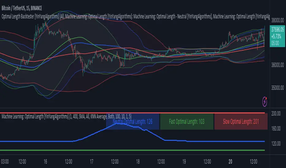
Backtest Strategy Optimizer AdapterBacktest Strategy Optimizer Adapter
With this library, you will be able to run one or multiple backtests with different variables (combinations). For example, you can run 100 backtests of Supertrend at once with an increment factor of 0.1. This way, you can easily fetch the most profitable settings and apply them to your strategy.
To get a better understanding of the code, you can check the code below.
Single backtest results
= backtest.results(date_start, date_end, long_entry, long_exit, take_profit_percentage, stop_loss_percentage, atr_length, initial_capital, order_size, commission)
Add backtest results to a table
backtest.table(initial_capital, profit_and_loss, open_balance, winrate, entries, exits, wins, losses, backtest_table_position, backtest_table_margin, backtest_table_transparency, backtest_table_cell_color, backtest_table_title_cell_color, backtest_table_text_color)
Backtest result without chart labels
= backtest.run(date_start, date_end, long_entry, long_exit, take_profit_percentage, stop_loss_percentage, atr_length, initial_capital, order_size, commission)
Backtest result profit
profit = backtest.profit(date_start, date_end, long_entry, long_exit, take_profit_percentage, stop_loss_percentage, atr_length, initial_capital, order_size, commission)
Backtest result winrate
winrate = backtest.winrate(date_start, date_end, long_entry, long_exit, take_profit_percentage, stop_loss_percentage, atr_length, initial_capital, order_size, commission)
Start Date
You can set the start date either by using a timestamp or a number that refers to the number of bars back.
Stop Loss / Take Profit Issue
Unfortunately, I did not manage to achieve 100% accuracy for the take profit and stop loss. The original TradingView backtest can stop at the correct position within a bar using the strategy.exit stop and limit variables. However, it seems unachievable with a crossunder/crossover function in PineScript unless it is calculated on every tick (which would make the backtesting results invalid). So far, I have not found a workaround, and I would be grateful if someone could solve this issue, if it is even possible. If you have any solutions or fixes, please let me know!
Multiple Backtest Results / Optimizer
You can run multiple backtests in a single strategy or indicator, but there are certain requirements for placing the correct code in the right way. To view examples of running multiple backtests, you can refer to the links provided in the updates I posted below. In the samples I have also explained how you can auto-generate code for your backtest strategy.
Machine Learning: Anchored Gaussian Process Regression [LuxAlgo]Machine Learning: Anchored Gaussian Process Regression is an anchored version of Machine Learning: Gaussian Process Regression .
It implements Gaussian Process Regression (GPR), a popular machine-learning method capable of estimating underlying trends in prices as well as forecasting them. Users can set a Training Window by choosing 2 points. GPR will be calculated for the data between these 2 points.
Do remember that forecasting trends in the market is challenging, do not use this tool as a standalone for your trading decisions.
🔶 USAGE
When adding the indicator to the chart, users will be prompted to select a starting and ending point for the calculations, click on your chart to select those points.
Start & end point are named 'Anchor 1' & 'Anchor 2', the Training Window is located between these 2 points. Once both points are positioned, the Training Window is set, whereafter the Gaussian Process Regression (GPR) is calculated using data between both Anchors .
The blue line is the GPR fit, the red line is the GPR prediction, derived from data between the Training Window .
Two user settings controlling the trend estimate are available, Smooth and Sigma.
Smooth determines the smoothness of our estimate, with higher values returning smoother results suitable for longer-term trend estimates.
Sigma controls the amplitude of the forecast, with values closer to 0 returning results with a higher amplitude.
One of the advantages of the anchoring process is the ability for the user to evaluate the accuracy of forecasts and further understand how settings affect their accuracy.
The publication also shows the mean average (faint silver line), which indicates the average of the prices within the calculation window (between the anchors). This can be used as a reference point for the forecast, seeing how it deviates from the training window average.
🔶 DETAILS
🔹 Limited Training Window
The Training Window is limited due to matrix.new() limitations in size.
When the 2 points are too far from each other (as in the latter example), the line will end at the maximum limit, without giving a size error.
The red forecasted line is always given priority.
🔹 Positioning Anchors
Typically Anchor 1 is located further in history than Anchor 2 , however, placing Anchor 2 before Anchor 1 is perfectly possibly, and won't give issues.
🔶 SETTINGS
Anchor 1 / Anchor 2: both points will form the Training Window .
Forecasting Length: Forecasting horizon, determines how many bars in the 'future' are forecasted.
Smooth: Controls the degree of smoothness of the model fit.
Sigma: Noise variance. Controls the amplitude of the forecast, lower values will make it more sensitive to outliers.
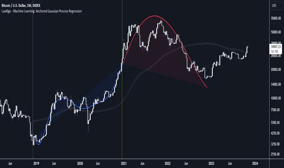
Machine Learning: VWAP [YinYangAlgorithms]Machine Learning: VWAP aims to use Machine Learning to Identify the best location to Anchor the VWAP at. Rather than using a traditional fixed length or simply adjusting based on a Date / Time; by applying Machine Learning we may hope to identify crucial areas which make sense to reset the VWAP and start anew. VWAP’s may act similar to a Bollinger Band in the sense that they help to identify both Overbought and Oversold Price locations based on previous movements and help to identify how far the price may move within the current Trend. However, unlike Bollinger Bands, VWAPs have the ability to parabolically get quite spaced out and also reset. For this reason, the price may never actually go from the Lower to the Upper and vice versa (when very spaced out; when the Upper and Lower zones are narrow, it may bounce between the two). The reason for this is due to how the anchor location is calculated and in this specific Indicator, how it changes anchors based on price movement calculated within Machine Learning.
This Indicator changes the anchor if the Low < Lowest Low of a length of X and likewise if the High > Highest High of a length of X. This logic is applied within a Machine Learning standpoint that likewise amplifies this Lookback Length by adding a Machine Learning Length to it and increasing the lookback length even further.
Due to how the anchor for this VWAP changes, you may notice that the Basis Line (Orange) may act as a Trend Identifier. When the Price is above the basis line, it may represent a bullish trend; and likewise it may represent a bearish trend when below it. You may also notice what may happen is when the trend occurs, it may push all the way to the Upper or Lower levels of this VWAP. It may then proceed to move horizontally until the VWAP expands more and it may gain more movement; or it may correct back to the Basis Line. If it corrects back to the basis line, what may happen is it either uses the Basis Line as a Support and continues in its current direction, or it will change the VWAP anchor and start anew.
Tutorial:
If we zoom in on the most recent VWAP we can see how it expands. Expansion may be caused by time but generally it may be caused by price movement and volume. Exponential Price movement causes the VWAP to expand, even if there are corrections to it. However, please note Volume adds a large weighted factor to the calculation; hence Volume Weighted Average Price (VWAP).
If you refer to the white circle in the example above; you’ll be able to see that the VWAP expanded even while the price was correcting to the Basis line. This happens due to exponential movement which holds high volume. If you look at the volume below the white circle, you’ll notice it was very large; however even though there was exponential price movement after the white circle, since the volume was low, the VWAP didn’t expand much more than it already had.
There may be times where both Volume and Price movement isn’t significant enough to cause much of an expansion. During this time it may be considered to be in a state of consolidation. While looking at this example, you may also notice the color switch from red to green to red. The color of the VWAP is related to the movement of the Basis line (Orange middle line). When the current basis is > the basis of the previous bar the color of the VWAP is green, and when the current basis is < the basis of the previous bar, the color of the VWAP is red. The color may help you gauge the current directional movement the price is facing within the VWAP.
You may have noticed there are signals within this Indicator. These signals are composed of Green and Red Triangles which represent potential Bullish and Bearish momentum changes. The Momentum changes happen when the Signal Type:
The High/Low or Close (You pick in settings)
Crosses one of the locations within the VWAP.
Bullish Momentum change signals occur when :
Signal Type crosses OVER the Basis
Signal Type crosses OVER the lower level
Bearish Momentum change signals occur when:
Signal Type crosses UNDER the Basis
Signal Type Crosses UNDER the upper level
These signals may represent locations where momentum may occur in the direction of these signals. For these reasons there are also alerts available to be set up for them.
If you refer to the two circles within the example above, you may see that when the close goes above the basis line, how it mat represents bullish momentum. Likewise if it corrects back to the basis and the basis acts as a support, it may continue its bullish momentum back to the upper levels again. However, if you refer to the red circle, you’ll see if the basis fails to act as a support, it may then start to correct all the way to the lower levels, or depending on how expanded the VWAP is, it may just reset its anchor due to such drastic movement.
You also have the ability to disable Machine Learning by setting ‘Machine Learning Type’ to ‘None’. If this is done, it will go off whether you have it set to:
Bullish
Bearish
Neutral
For the type of VWAP you want to see. In this example above we have it set to ‘Bullish’. Non Machine Learning VWAP are still calculated using the same logic of if low < lowest low over length of X and if high > highest high over length of X.
Non Machine Learning VWAP’s change much quicker but may also allow the price to correct from one side to the other without changing VWAP Anchor. They may be useful for breaking up a trend into smaller pieces after momentum may have changed.
Above is an example of how the Non Machine Learning VWAP looks like when in Bearish. As you can see based on if it is Bullish or Bearish is how it favors the trend to be and may likewise dictate when it changes the Anchor.
When set to neutral however, the Anchor may change quite quickly. This results in a still useful VWAP to help dictate possible zones that the price may move within, but they’re also much tighter zones that may not expand the same way.
We will conclude this Tutorial here, hopefully this gives you some insight as to why and how Machine Learning VWAPs may be useful; as well as how to use them.
Settings:
VWAP:
VWAP Type: Type of VWAP. You can favor specific direction changes or let it be Neutral where there is even weight to both. Please note, these do not apply to the Machine Learning VWAP.
Source: VWAP Source. By default VWAP usually uses HLC3; however OHLC4 may help by providing more data.
Lookback Length: The Length of this VWAP when it comes to seeing if the current High > Highest of this length; or if the current Low is < Lowest of this length.
Standard VWAP Multiplier: This multiplier is applied only to the Standard VWMA. This is when 'Machine Learning Type' is set to 'None'.
Machine Learning:
Use Rational Quadratics: Rationalizing our source may be beneficial for usage within ML calculations.
Signal Type: Bullish and Bearish Signals are when the price crosses over/under the basis, as well as the Upper and Lower levels. These may act as indicators to where price movement may occur.
Machine Learning Type: Are we using a Simple ML Average, KNN Mean Average, KNN Exponential Average or None?
KNN Distance Type: We need to check if distance is within the KNN Min/Max distance, which distance checks are we using.
Machine Learning Length: How far back is our Machine Learning going to keep data for.
k-Nearest Neighbour (KNN) Length: How many k-Nearest Neighbours will we account for?
Fast ML Data Length: What is our Fast ML Length? This is used with our Slow Length to create our KNN Distance.
Slow ML Data Length: What is our Slow ML Length? This is used with our Fast Length to create our KNN Distance.
If you have any questions, comments, ideas or concerns please don't hesitate to contact us.
HAPPY TRADING!

Machine Learning: Optimal RSI [YinYangAlgorithms]This Indicator, will rate multiple different lengths of RSIs to determine which RSI to RSI MA cross produced the highest profit within the lookback span. This ‘Optimal RSI’ is then passed back, and if toggled will then be thrown into a Machine Learning calculation. You have the option to Filter RSI and RSI MA’s within the Machine Learning calculation. What this does is, only other Optimal RSI’s which are in the same bullish or bearish direction (is the RSI above or below the RSI MA) will be added to the calculation.
You can either (by default) use a Simple Average; which is essentially just a Mean of all the Optimal RSI’s with a length of Machine Learning. Or, you can opt to use a k-Nearest Neighbour (KNN) calculation which takes a Fast and Slow Speed. We essentially turn the Optimal RSI into a MA with different lengths and then compare the distance between the two within our KNN Function.
RSI may very well be one of the most used Indicators for identifying crucial Overbought and Oversold locations. Not only that but when it crosses its Moving Average (MA) line it may also indicate good locations to Buy and Sell. Many traders simply use the RSI with the standard length (14), however, does that mean this is the best length?
By using the length of the top performing RSI and then applying some Machine Learning logic to it, we hope to create what may be a more accurate, smooth, optimal, RSI.
Tutorial:
This is a pretty zoomed out Perspective of what the Indicator looks like with its default settings (except with Bollinger Bands and Signals disabled). If you look at the Tables above, you’ll notice, currently the Top Performing RSI Length is 13 with an Optimal Profit % of: 1.00054973. On its default settings, what it does is Scan X amount of RSI Lengths and checks for when the RSI and RSI MA cross each other. It then records the profitability of each cross to identify which length produced the overall highest crossing profitability. Whichever length produces the highest profit is then the RSI length that is used in the plots, until another length takes its place. This may result in what we deem to be the ‘Optimal RSI’ as it is an adaptive RSI which changes based on performance.
In our next example, we changed the ‘Optimal RSI Type’ from ‘All Crossings’ to ‘Extremity Crossings’. If you compare the last two examples to each other, you’ll notice some similarities, but overall they’re quite different. The reason why is, the Optimal RSI is calculated differently. When using ‘All Crossings’ everytime the RSI and RSI MA cross, we evaluate it for profit (short and long). However, with ‘Extremity Crossings’, we only evaluate it when the RSI crosses over the RSI MA and RSI <= 40 or RSI crosses under the RSI MA and RSI >= 60. We conclude the crossing when it crosses back on its opposite of the extremity, and that is how it finds its Optimal RSI.
The way we determine the Optimal RSI is crucial to calculating which length is currently optimal.
In this next example we have zoomed in a bit, and have the full default settings on. Now we have signals (which you can set alerts for), for when the RSI and RSI MA cross (green is bullish and red is bearish). We also have our Optimal RSI Bollinger Bands enabled here too. These bands allow you to see where there may be Support and Resistance within the RSI at levels that aren’t static; such as 30 and 70. The length the RSI Bollinger Bands use is the Optimal RSI Length, allowing it to likewise change in correlation to the Optimal RSI.
In the example above, we’ve zoomed out as far as the Optimal RSI Bollinger Bands go. You’ll notice, the Bollinger Bands may act as Support and Resistance locations within and outside of the RSI Mid zone (30-70). In the next example we will highlight these areas so they may be easier to see.
Circled above, you may see how many times the Optimal RSI faced Support and Resistance locations on the Bollinger Bands. These Bollinger Bands may give a second location for Support and Resistance. The key Support and Resistance may still be the 30/50/70, however the Bollinger Bands allows us to have a more adaptive, moving form of Support and Resistance. This helps to show where it may ‘bounce’ if it surpasses any of the static levels (30/50/70).
Due to the fact that this Indicator may take a long time to execute and it can throw errors for such, we have added a Setting called: Adjust Optimal RSI Lookback and RSI Count. This settings will automatically modify the Optimal RSI Lookback Length and the RSI Count based on the Time Frame you are on and the Bar Indexes that are within. For instance, if we switch to the 1 Hour Time Frame, it will adjust the length from 200->90 and RSI Count from 30->20. If this wasn’t adjusted, the Indicator would Timeout.
You may however, change the Setting ‘Adjust Optimal RSI Lookback and RSI Count’ to ‘Manual’ from ‘Auto’. This will give you control over the ‘Optimal RSI Lookback Length’ and ‘RSI Count’ within the Settings. Please note, it will likely take some “fine tuning” to find working settings without the Indicator timing out, but there are definitely times you can find better settings than our ‘Auto’ will create; especially on higher Time Frames. The Minimum our ‘Auto’ will create is:
Optimal RSI Lookback Length: 90
RSI Count: 20
The Maximum it will create is:
Optimal RSI Lookback Length: 200
RSI Count: 30
If there isn’t much bar index history, for instance, if you’re on the 1 Day and the pair is BTC/USDT you’ll get < 4000 Bar Indexes worth of data. For this reason it is possible to manually increase the settings to say:
Optimal RSI Lookback Length: 500
RSI Count: 50
But, please note, if you make it too high, it may also lead to inaccuracies.
We will conclude our Tutorial here, hopefully this has given you some insight as to how calculating our Optimal RSI and then using it within Machine Learning may create a more adaptive RSI.
Settings:
Optimal RSI:
Show Crossing Signals: Display signals where the RSI and RSI Cross.
Show Tables: Display Information Tables to show information like, Optimal RSI Length, Best Profit, New Optimal RSI Lookback Length and New RSI Count.
Show Bollinger Bands: Show RSI Bollinger Bands. These bands work like the TDI Indicator, except its length changes as it uses the current RSI Optimal Length.
Optimal RSI Type: This is how we calculate our Optimal RSI. Do we use all RSI and RSI MA Crossings or just when it crosses within the Extremities.
Adjust Optimal RSI Lookback and RSI Count: Auto means the script will automatically adjust the Optimal RSI Lookback Length and RSI Count based on the current Time Frame and Bar Index's on chart. This will attempt to stop the script from 'Taking too long to Execute'. Manual means you have full control of the Optimal RSI Lookback Length and RSI Count.
Optimal RSI Lookback Length: How far back are we looking to see which RSI length is optimal? Please note the more bars the lower this needs to be. For instance with BTC/USDT you can use 500 here on 1D but only 200 for 15 Minutes; otherwise it will timeout.
RSI Count: How many lengths are we checking? For instance, if our 'RSI Minimum Length' is 4 and this is 30, the valid RSI lengths we check is 4-34.
RSI Minimum Length: What is the RSI length we start our scans at? We are capped with RSI Count otherwise it will cause the Indicator to timeout, so we don't want to waste any processing power on irrelevant lengths.
RSI MA Length: What length are we using to calculate the optimal RSI cross' and likewise plot our RSI MA with?
Extremity Crossings RSI Backup Length: When there is no Optimal RSI (if using Extremity Crossings), which RSI should we use instead?
Machine Learning:
Use Rational Quadratics: Rationalizing our Close may be beneficial for usage within ML calculations.
Filter RSI and RSI MA: Should we filter the RSI's before usage in ML calculations? Essentially should we only use RSI data that are of the same type as our Optimal RSI? For instance if our Optimal RSI is Bullish (RSI > RSI MA), should we only use ML RSI's that are likewise bullish?
Machine Learning Type: Are we using a Simple ML Average, KNN Mean Average, KNN Exponential Average or None?
KNN Distance Type: We need to check if distance is within the KNN Min/Max distance, which distance checks are we using.
Machine Learning Length: How far back is our Machine Learning going to keep data for.
k-Nearest Neighbour (KNN) Length: How many k-Nearest Neighbours will we account for?
Fast ML Data Length: What is our Fast ML Length? This is used with our Slow Length to create our KNN Distance.
Slow ML Data Length: What is our Slow ML Length? This is used with our Fast Length to create our KNN Distance.
If you have any questions, comments, ideas or concerns please don't hesitate to contact us.
HAPPY TRADING!
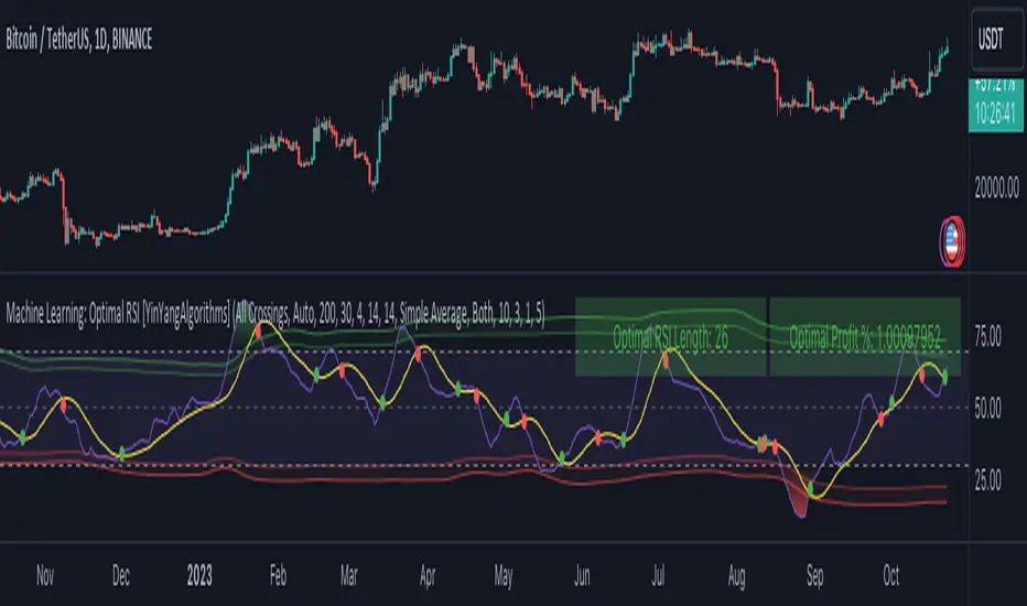
Machine Learning: SuperTrend Strategy TP/SL [YinYangAlgorithms]The SuperTrend is a very useful Indicator to display when trends have shifted based on the Average True Range (ATR). Its underlying ideology is to calculate the ATR using a fixed length and then multiply it by a factor to calculate the SuperTrend +/-. When the close crosses the SuperTrend it changes direction.
This Strategy features the Traditional SuperTrend Calculations with Machine Learning (ML) and Take Profit / Stop Loss applied to it. Using ML on the SuperTrend allows for the ability to sort data from previous SuperTrend calculations. We can filter the data so only previous SuperTrends that follow the same direction and are within the distance bounds of our k-Nearest Neighbour (KNN) will be added and then averaged. This average can either be achieved using a Mean or with an Exponential calculation which puts added weight on the initial source. Take Profits and Stop Losses are then added to the ML SuperTrend so it may capitalize on Momentum changes meanwhile remaining in the Trend during consolidation.
By applying Machine Learning logic and adding a Take Profit and Stop Loss to the Traditional SuperTrend, we may enhance its underlying calculations with potential to withhold the trend better. The main purpose of this Strategy is to minimize losses and false trend changes while maximizing gains. This may be achieved by quick reversals of trends where strategic small losses are taken before a large trend occurs with hopes of potentially occurring large gain. Due to this logic, the Win/Loss ratio of this Strategy may be quite poor as it may take many small marginal losses where there is consolidation. However, it may also take large gains and capitalize on strong momentum movements.
Tutorial:
In this example above, we can get an idea of what the default settings may achieve when there is momentum. It focuses on attempting to hit the Trailing Take Profit which moves in accord with the SuperTrend just with a multiplier added. When momentum occurs it helps push the SuperTrend within it, which on its own may act as a smaller Trailing Take Profit of its own accord.
We’ve highlighted some key points from the last example to better emphasize how it works. As you can see, the White Circle is where profit was taken from the ML SuperTrend simply from it attempting to switch to a Bullish (Buy) Trend. However, that was rejected almost immediately and we went back to our Bearish (Sell) Trend that ended up resulting in our Take Profit being hit (Yellow Circle). This Strategy aims to not only capitalize on the small profits from SuperTrend to SuperTrend but to also capitalize when the Momentum is so strong that the price moves X% away from the SuperTrend and is able to hit the Take Profit location. This Take Profit addition to this Strategy is crucial as momentum may change state shortly after such drastic price movements; and if we were to simply wait for it to come back to the SuperTrend, we may lose out on lots of potential profit.
If you refer to the Yellow Circle in this example, you’ll notice what was talked about in the Summary/Overview above. During periods of consolidation when there is little momentum and price movement and we don’t have any Stop Loss activated, you may see ‘Signal Flashing’. Signal Flashing is when there are Buy and Sell signals that keep switching back and forth. During this time you may be taking small losses. This is a normal part of this Strategy. When a signal has finally been confirmed by Momentum, is when this Strategy shines and may produce the profit you desire.
You may be wondering, what causes these jagged like patterns in the SuperTrend? It's due to the ML logic, and it may be a little confusing, but essentially what is happening is the Fast Moving SuperTrend and the Slow Moving SuperTrend are creating KNN Min and Max distances that are extreme due to (usually) parabolic movement. This causes fewer values to be added to and averaged within the ML and causes less smooth and more exponential drastic movements. This is completely normal, and one of the perks of using k-Nearest Neighbor for ML calculations. If you don’t know, the Min and Max Distance allowed is derived from the most recent(0 index of data array) to KNN Length. So only SuperTrend values that exhibit distances within these Min/Max will be allowed into the average.
Since the KNN ML logic can cause these exponential movements in the SuperTrend, they likewise affect its Take Profit. The Take Profit may benefit from this movement like displayed in the example above which helped it claim profit before then exhibiting upwards movement.
By default our Stop Loss Multiplier is kept quite low at 0.0000025. Keeping it low may help to reduce some Signal Flashing while not taking extra losses more so than not using it at all. However, if we increase it even more to say 0.005 like is shown in the example above. It can really help the trend keep momentum. Please note, although previous results don’t imply future results, at 0.0000025 Stop Loss we are currently exhibiting 69.27% profit while at 0.005 Stop Loss we are exhibiting 33.54% profit. This just goes to show that although there may be less Signal Flashing, it may not result in more profit.
We will conclude our Tutorial here. Hopefully this has given you some insight as to how Machine Learning, combined with Trailing Take Profit and Stop Loss may have positive effects on the SuperTrend when turned into a Strategy.
Settings:
SuperTrend:
ATR Length: ATR Length used to create the Original Supertrend.
Factor: Multiplier used to create the Original Supertrend.
Stop Loss Multiplier: 0 = Don't use Stop Loss. Stop loss can be useful for helping to prevent false signals but also may result in more loss when hit and less profit when switching trends.
Take Profit Multiplier: Take Profits can be useful within the Supertrend Strategy to stop the price reverting all the way to the Stop Loss once it's been profitable.
Machine Learning:
Only Factor Same Trend Direction: Very useful for ensuring that data used in KNN is not manipulated by different SuperTrend Directional data. Please note, it doesn't affect KNN Exponential.
Rationalized Source Type: Should we Rationalize only a specific source, All or None?
Machine Learning Type: Are we using a Simple ML Average, KNN Mean Average, KNN Exponential Average or None?
Machine Learning Smoothing Type: How should we smooth our Fast and Slow ML Datas to be used in our KNN Distance calculation? SMA, EMA or VWMA?
KNN Distance Type: We need to check if distance is within the KNN Min/Max distance, which distance checks are we using.
Machine Learning Length: How far back is our Machine Learning going to keep data for.
k-Nearest Neighbour (KNN) Length: How many k-Nearest Neighbours will we account for?
Fast ML Data Length: What is our Fast ML Length?? This is used with our Slow Length to create our KNN Distance.
Slow ML Data Length: What is our Slow ML Length?? This is used with our Fast Length to create our KNN Distance.
If you have any questions, comments, ideas or concerns please don't hesitate to contact us.
HAPPY TRADING!
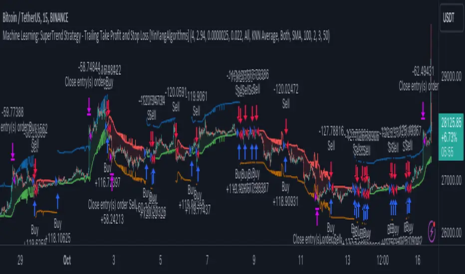
Machine Learning using Neural Networks | EducationalThe script provided is a comprehensive illustration of how to implement and execute a simplistic Neural Network (NN) on TradingView using PineScript.
It encompasses the entire workflow from data input, weight initialization, implicit neuron calculation, feedforward computation, backpropagation for weight adjustments, generating predictions, to visualizing the Mean Squared Error (MSE) Loss Curve for monitoring the training phase.
In the visual example above, you can see that the prediction is not aligned with the actual value. This is intentional for demonstrative purposes, and by incrementing the Epochs or Learning Rate, you will see these two values converge as the accuracy increases.
Hyperparameters:
Learning Rate, Epochs, and the choice between Simple Backpropagation and a verbose version are declared as script inputs, allowing users to tailor the training process.
Initialization:
Random initialization of weight matrices (w1, w2) is performed to ensure asymmetry, promoting effective gradient updates. A seed is added for reproducibility.
Utility Functions:
Functions for matrix randomization, sigmoid activation, MSE loss calculation, data normalization, and standardization are defined to streamline the computation process.
Neural Network Computation:
The feedforward function computes the hidden and output layer values given the input.
Two variants of the backpropagation function are provided for weight adjustment, with one offering a more verbose step-by-step computation of gradients.
A wrapper train_nn function iterates through epochs, performing feedforward, loss computation, and backpropagation in each epoch while logging and collecting loss values.
Training Invocation:
The input data is prepared by normalizing it to a value between 0 and 1 using the maximum standardized value, and the training process is invoked only on the last confirmed bar to preserve computational resources.
Output Forecasting and Visualization:
Post training, the NN's output (predicted price) is computed, standardized and visualized alongside the actual price on the chart.
The MSE loss between the predicted and actual prices is visualized, providing insight into the prediction accuracy.
Optionally, the MSE Loss Curve is plotted on the chart, illustrating the loss trajectory through epochs, assisting in understanding the training performance.
Customizable Visualization:
Various inputs control visualization aspects like Chart Scaling, Chart Horizontal Offset, and Chart Vertical Offset, allowing users to adapt the visualization to their preference.
-------------------------------------------------------
The following is this Neural Network structure, consisting of one hidden layer, with two hidden neurons.
Through understanding the steps outlined in my code, one should be able to scale the NN in any way they like, such as changing the input / output data and layers to fit their strategy ideas.
Additionally, one could forgo the backpropagation function, and load their own trained weights into the w1 and w2 matrices, to have this code run purely for inference.
-------------------------------------------------------
While this demonstration does create a “prediction”, it is on historical data. The purpose here is educational, rather than providing a ready tool for non-programmer consumers.
Normally in Machine Learning projects, the training process would be split into two segments, the Training and the Validation parts. For the purpose of conveying the core concept in a concise and non-repetitive way, I have foregone the Validation part. However, it is merely the application of your trained network on new data (feedforward), and monitoring the loss curve.
Essentially, checking the accuracy on “unseen” data, while training it on “seen” data.
-------------------------------------------------------
I hope that this code will help developers create interesting machine learning applications within the Tradingview ecosystem.
