VectorCoresAI SMA + Bollinger Fusion v1VectorCoresAI — SMA + Bollinger Fusion (Free)
A clean, modern visual tool combining four key SMAs with an adaptive Bollinger structure.
This script merges two of the most widely used charting concepts into one simple, readable view:
Included
✔ SMA 21
✔ SMA 50
✔ SMA 100
✔ SMA 200
✔ Bollinger Bands with adjustable length + multiplier
✔ Adaptive “Fusion Squeeze” shading to highlight compression phases
✔ Optional visibility toggles for each SMA
✔ Lightweight, non-intrusive overlay
What this indicator is designed for
This tool helps traders quickly understand:
Trend alignment using the 21/50/100/200 SMAs
Volatility conditions around the Bollinger midline
Price compression and expansion
Early awareness of breakout environments
Clean visual structure without clutter
Everything is intentionally simple and transparent.
No predictions, no signals, no trading advice — just clean chart structure.
Why this version is unique
Instead of using standard Bollinger visuals, this Fusion edition uses subtle adaptive shading to show when the bands contract.
This makes compression zones instantly visible without overwhelming the chart.
The SMAs are fixed to widely-used trend levels, giving consistent readings across all markets and timeframes.
Who this is for
Newer traders who want a clear introduction to SMAs + Bollinger Bands
Experienced traders who want a lightweight visual tool
Anyone building structure-based strategies
Users of the VectorCoresAI suite who want a simple companion tool
Notes
This indicator is part of the VectorCoresAI Free Tools collection.
All logic is open-source and educational only.
More tools coming soon.
Bollingerbandstrategy

Bollinger Bands Mean Reversion using RSI [Krishna Peri]How it Works
Long entries trigger when:
- RSI reaches oversold levels, and
- At least one bullish candle closes inside the lower Bollinger Band
Short entries trigger when:
- RSI reaches overbought levels, and
- At least one bearish candle closes inside the upper Bollinger Band
This approach aims to capture exhaustion moves where price pushes into extreme deviation from its mean and then snaps back toward the middle band.
Important Disclaimer
This is a mean-reversion strategy, which means it performs best in sideways, ranging, or slowly oscillating market conditions. When markets shift into strong trends, Bollinger Bands expand and volatility increases, which may cause some signals to become inaccurate or fail altogether.
For best results, combine this script with:
- Price action
- Market structure
- Higher-timeframe trend context
- Previous day/week/month highs & lows
- Untested liquidity levels or imbalance zones
- Session timing (Asia, London, NY)
Using these confluences helps filter out low-probability trades and significantly improves consistency and precision.
Center and Volume AnalyzerCenter and Volume Analyzer that utilizes the chart's Center of Gravity alongside the Rate of Change with Bollinger Bands with a basis for the midpoint. As always, none of this is investment or financial advice. Please do your own due diligence and research.

Pro Bollinger Bands Strategy [Breno]This strategy excels in highly volatile financial instruments, including cryptocurrencies, high-beta stocks, commodity futures, and certain exchange-traded funds (ETFs) that exhibit clear mean-reversion characteristics around their Bollinger Bands. The system's ability to utilize scaling (position averaging) and an ATR-based stop loss makes it particularly effective in markets with significant price swings, allowing the trader to capture profits from price extremes while managing increased volatility-related risk.
Core Strategy Logic
This Strategy implements a comprehensive trend-following and mean-reversion strategy primarily leveraging the Bollinger Bands (BB) indicator for entry and exit signals, complemented by an Average True Range (ATR)-based Stop Loss mechanism and an optional EMA filter. It is designed with robust features for capital management, including configurable leverage and a sophisticated position averaging (scaling) system.
Long Entry: A long position is initiated when the closing price crosses over the Lower Bollinger Band (ta.crossover(close,lowerBB)). This signals a potential mean-reversion opportunity following a price dip.
Short Entry: A short position is initiated when the closing price crosses under the Upper Bollinger Band (ta.crossunder(close,upperBB)). (Note: Short entries are disabled by default in the script inputs).
Exit Conditions (Profit Target): Long positions aim to exit upon interaction with the Upper Bollinger Band. Users can select from three exit methods:
"Close When Touch": Exits when close≥upperBB.
"Close Above then Below": Exits when the previous close was above the upper band, and the current close is below it (a reversal signal).
"High Above": Exits when high>upperBB. The strategy features an optional profitOnly setting, which restricts all exits to only occur if the trade is currently in profit (i.e., close is above the strategy.position_avg_price for longs).
Key Features and Customization
Bollinger Bands & Filters -
Customizable BB Parameters: The Length and Deviation of the Bollinger Bands are fully adjustable, allowing users to fine-tune the sensitivity of the entry and exit signals.
Optional EMA Filter: An optional EMA Filter can be enabled to align entries with the prevailing trend, where a Long entry is only permitted if close≥EMA(EmaFilterRange).
Risk and Capital Management -
Equity Allocation: Position size is dynamically calculated based on a Percentage of Equity (capitalPerc) combined with the set Leverage multiplier.
Dynamic Stop Loss (ATR-Based):
An optional Stop Loss (SL) is calculated using a multiple (slAtrInput) of the Average True Range (ATR).
The SL is set relative to the entry price upon trade activation, providing a volatility-adjusted risk management layer.
Position Averaging (Scaling): The script supports the addition of multiple units (pyramiding) to an existing position based on three user-selected criteria:
"No": No averaging.
"Percent": Adds to the position if the price has dropped by a set percentage (addPct) from the average price.
"ATR": Adds to the position if the current price is significantly below a calculated ATR-based support level from the average price.

Bollinger Bands Delta Matrix Analytics [BDMA] Bollinger Bands Delta Matrix Analytics (BDMA) v7.0
Deep Kinetic Engine – 5x8 Volatility & Delta Decision Matrix
1. Introduction & Concept
Bollinger Bands Delta Matrix Analytics (BDMA) v7.0 is an analytical framework that merges:
- Spatial analysis via Bollinger Bands (%B location),
- with a 4-factor Deep Kinetic Engine based on:
• Total Volume
• Buy Volume
• Sell Volume
• Delta (Buy – Sell) Z-Scores
and converts them into an expanded 5×8 decision matrix that continuously tracks where price is trading and how the underlying orderflow is behaving.
BDMA is not a trading system or strategy. It does not generate entry/exit signals.
Instead, it provides a structured contextual map of volatility, volume, and delta so traders can:
- identify climactic extensions vs. fakeouts,
- distinguish strong initiative moves vs. passive absorption,
- and detect squeezes, traps, and liquidity voids with a unified visual dashboard.
2. Spatial Engine – Bollinger S-States (S1–S5)
The spatial dimension of BDMA comes from classic Bollinger Bands.
Price location is expressed as Percent B (%B) and mapped into 5 spatial states (S-States):
S1 – Hyper Extension (Above Upper Band)
Price has pushed beyond the upper Bollinger Band.
Often associated with parabolic or blow-off behavior, late-stage momentum, and elevated reversal risk.
S2 – Resistance Test (Upper Zone)
Price trades in the upper Bollinger region but remains inside the bands.
Represents a sustained test of resistance, typically within an established or emerging uptrend.
S3 – Neutral Zone (Middle)
Price hovers around the mid-band.
This is the mean reversion gravity field where the market often consolidates or transitions between regimes.
S4 – Support Test (Lower Zone)
Price trades in the lower Bollinger region but inside the bands.
Represents a sustained test of support within range or downtrend structures.
S5 – Hyper Drop (Below Lower Band)
Price extends below the lower Bollinger Band.
Often aligned with panic, forced liquidations, or capitulation-type behavior, with increased snap-back risk.
These 5 S-States define the vertical axis (rows) of the BDMA matrix.
3. Deep Kinetic Engine – 4-Factor Z-Score & D-States (D1–D8)
The Deep Kinetic Engine transforms raw volume and delta into standardized Z-Scores to measure how abnormal current activity is relative to its recent history.
For each bar:
- Raw Buy Volume is estimated from the candle’s position within its range
- Raw Sell Volume is complementary to buy volume
- Raw Delta = Buy Volume – Sell Volume
- Total Volume = Buy Volume + Sell Volume
These 4 series are then normalized using a unified Z-Score lookback to produce:
1. Z_Vol_Total – overall activity and liquidity intensity
2. Z_Vol_Buy – aggression from buyers (attack)
3. Z_Vol_Sell – aggression from sellers (defense or attack)
4. Z_Delta – net victory of one side over the other
Thresholds for Extreme, Significant, and Neutral Z-Score levels are fully configurable, allowing you to tune the sensitivity of the kinetic states.
Using Z_Vol_Total and Z_Delta (plus threshold logic), BDMA assigns one of 8 Deep Kinetic states (D-States):
D1 – Climax Buy
Extreme Total Volume + Extreme Positive Delta → Buying climax or blow-off behavior.
D2 – Strong Buy
High Volume + High Positive Delta → Confirmed bullish initiative activity.
D3 – Weak Buy / Fakeout
Low Volume + High Positive Delta → Bullish delta without commitment, low-liquidity breakout risk.
D4 – Absorption / Conflict
High Volume + Neutral Delta → Aggressive two-way trade, strong absorption, war zone behavior.
D5 – Neutral
Low Volume + Neutral Delta → Low-energy environment with low conviction.
D6 – Weak Sell / Fakeout
Low Volume + High Negative Delta → Bearish delta without commitment, low-liquidity breakdown risk.
D7 – Strong Sell
High Volume + High Negative Delta → Confirmed bearish initiative activity.
D8 – Capitulation
Extreme Volume + Extreme Negative Delta → Panic selling or capitulation regime.
These 8 D-States define the horizontal axis (columns) of the BDMA matrix.
4. The 5×8 BDMA Decision Matrix
The core of BDMA is a 5×8 matrix where:
- Rows (1–5) = Spatial S-States (S1…S5)
- Columns (1–8) = Kinetic D-States (D1…D8)
Each of the 40 possible combinations (SxDy) is pre-computed and mapped to:
- a Status or Regime Title (for example: Climax Breakout, Bear Trap Spring, Capitulation Breakdown),
- a Bias (Climactic Bull, Neutral, Strong Bear, Conflict or Reversal Risk, and similar labels),
- and a Strategic Signal or Consideration (for example: High reversal risk, Wait for confirmation, Low probability zone – avoid).
Internally, BDMA resolves all 40 regimes so the current state can be displayed on the dashboard without performance overhead.
5. Key Regime Families (How to Read the Matrix)
5.1. Breakouts and Breakdowns
Climax Breakout (Top-side)
Spatial S1 with Kinetic D1 or D2
Bias: Explosive or Extreme Bull
Signal:
- Strong or climactic upside extension with abnormal bullish orderflow.
- Trend continuation is possible, but reversal risk is extremely high after blow-off phases.
Low-Conviction Breakout (Fakeout Risk)
S1 with D3 (Weak Buy, low liquidity)
Bias: Weak Bull – Caution
Signal:
- Breakout not supported by volume.
- Elevated risk of failed auction or bull trap.
Capitulation Breakdown (Bottom-side)
Spatial S5 with Kinetic D8
Bias: Climactic Bear (panic)
Signal:
- Capitulation-type selling or forced liquidations.
- Trend can still proceed, but snap-back or violent short-covering risk is high.
Initiative Breakdown vs. Weak Breakdown
- Strong, high-volume breakdown typically corresponds to D7 (Strong Sell).
- Low-volume breakdown often corresponds to D6 (Weak Sell or Fakeout) with potential for failure.
5.2. Absorption, Traps and Springs
Absorption at Resistance (Top-side conflict)
S1 or S2 with D4 (Absorption or Conflict)
Bias: Conflict – Extreme Tension
Signal:
- Heavy two-way trade near resistance.
- Potential distribution or reversal if sellers begin to dominate.
Bull Trap or Failed Auction
Typically S1 with D6 (Weak Sell breakdown behavior after a top-side attempt)
Indicates a breakout attempt that fails and reverses, often after poor liquidity structure.
Absorption at Support and Bear Trap (Spring)
S4 or S5 with D4 or D3
Bias: Conflict or Weak Bear – Reversal Risk
Signal:
- Aggressive buying into lows (spring or shakeout behavior).
- Potential bear trap if price reclaims lost territory.
5.3. Trend Phases
Strong Uptrend Phases
Typically seen when S2–S3 combine with strong bullish kinetic behavior.
Bias: Strong or Extreme Bull
Signal:
- Pullbacks into S3 or S4 with supportive kinetic states often act as trend continuation zones.
Strong Downtrend Phases
Typically seen when S3–S4 combine with strong bearish kinetic behavior.
Bias: Strong or Extreme Bear
Signal:
- Rallies into resistance with strong bearish kinetic backing may act as continuation sell zones.
5.4. Neutral, Exhaustion and Squeeze
Exhaustion or Liquidity Void
S1 or S5 with D5 (Neutral kinetics)
Bias: Neutral or Exhaustion
Signal:
- Spatial extremes without kinetic confirmation.
- Often marks the end of a move, with poor follow-through.
Choppy, Low-Activity Range
S3 with D5
Bias: Neutral
Signal:
- Low volume, low conviction market.
- Typically a low-probability environment where standing aside can be logical.
Squeeze or High-Tension Zone
S3 with D4 or tightly clustered kinetic values
Bias: Conflict or High Tension
Signal:
- Hidden battle inside a volatility contraction.
- Often precedes large directionally-biased moves.
6. Dashboard Layout & Reading Guide
When Show Dashboard is enabled, BDMA displays:
1. Title and Status Line
Name of the current regime (for example: Climax Breakout, Bear Trap Spring, Mean Reversion).
2. Bias Line
Plain-language summary of directional context such as Climactic Bull, Strong Bear, Neutral, or Conflict and Reversal Risk.
3. Signal or Strategic Notes
Concise guidance focused on risk and context, not entries. For example:
- High reversal risk – aggressive traders only
- Wait for confirmation (break or rejection)
- Low probability zone – avoid taking new positions
4. Kinetic Profile (4-Factor Z-Score)
Shows the current Z-Scores for Total Volume (Activity), Buy Volume (Attack), Sell Volume (Defense), and Delta (Net Result).
5. Matrix Heatmap (5×8)
Visual representation of S-State vs. D-State with color coding:
- Bullish clusters in a green spectrum
- Bearish clusters in a red spectrum
- Conflict or exhaustion zones in yellow, amber, or neutral tones
The dashboard can be repositioned (top right, middle right, or bottom right) and its size can be adjusted (Tiny, Small, Normal, or Large) to fit different layouts.
7. Inputs & Customization
7.1. Core Parameters (Bollinger and Z-Score)
- Bollinger Length and Standard Deviation define the spatial engine.
- Z-Score Lookback (All Factors) defines how many bars are used to normalize volume and delta.
7.2. Deep Kinetic Thresholds
- Extreme Threshold defines what is considered climactic (D1 or D8).
- Significant Threshold distinguishes strong initiative vs. weak or fakeout behavior.
- Neutral Threshold is the band within which delta is treated as neutral.
These thresholds allow you to tune the sensitivity of the kinetic classification to fit different timeframes or instruments.
7.3. Calculation Method (Volume Delta)
Geometry (Approx)
- Fast, non-repainting approach based on candle geometry.
- Suitable for most users and real-time decision-making.
Intrabar (Precise)
- Uses lower-timeframe data for more precise volume delta estimation.
- Intrabar mode can repaint and requires compatible data and plan support on the platform.
- Best used for post-analysis or research, not blind automation.
7.4. Visuals and Interface
- Toggle Bollinger Bands visibility on or off.
- Switch between Dark and Light color themes.
- Configure dashboard visibility, matrix heatmap display, position, and size.
8. Multi-Language Semantic Engine (Asia and Middle East Focus)
BDMA v7.0 includes a fully integrated multi-language layer, targeting a wide geographic user base.
Supported Languages:
English, Türkçe, Русский, 简体中文, हिन्दी, العربية, فارسی, עברית
All dashboard labels, regime titles, bias descriptions, and signal texts are dynamically translated via an internal dictionary, while semantic meaning is kept consistent across languages.
This makes BDMA suitable for multi-language communities, study groups, and educational content across different regions.
However, due to the heavy computational load of the Deep Kinetic Engine and TradingView’s strict Pine Script execution limits, it was not possible to expand support to additional languages. Adding more translation layers would significantly increase memory usage and exceed runtime constraints. For this reason, the current language set represents the maximum optimized configuration achievable without compromising performance or stability.
9. Practical Usage Notes
BDMA is most powerful when used as a contextual overlay on top of market structure (HH, HL, LH, LL), higher-timeframe trend, key levels, and your own execution framework.
Recommended usage:
- Identify the current regime (Status and Bias).
- Check whether price location (S-State) and kinetic behavior (D-State) agree with your trade idea.
- Be especially cautious in climactic and absorption or conflict zones, where volatility and risk can be elevated.
Avoid treating BDMA as an automatic green equals buy, red equals sell tool.
The real edge comes from understanding where you are in the volatility or kinetic spectrum, not from forcing signals out of the matrix.
10. Limitations & Important Warnings
BDMA does not predict the future.
It organizes current and recent data into a structured context.
Volume data quality depends on the underlying symbol, exchange, and broker feed.
Forex, crypto, indices, and stocks may all behave differently.
Intrabar mode can repaint and is sensitive to lower-timeframe data availability and your plan type.
Use it with extra caution and primarily for research.
No indicator can remove the need for clear trading rules, disciplined risk management, and psychological control.
11. Disclaimer
This script is provided strictly for educational and analytical purposes.
It is not a trading system, signal service, financial product, or investment advice.
Nothing in this indicator or its description should be interpreted as a recommendation to buy or sell any asset.
Past behavior of any indicator or market pattern does not guarantee future results.
Trading and investing involve significant risk, including the risk of losing more than your initial capital in leveraged products.
You are solely responsible for your own decisions, risk management, and results.
By using this script, you acknowledge that you understand these risks and agree that the author or authors and publisher or publishers are not liable for any loss or damage arising from its use.

Filte Ichimoku1. Indicator Name
Filte Ichimoku
2. One-line Introduction
A smoothed and visually enhanced version of the Ichimoku Cloud that highlights trend direction and strength using adaptive color transparency.
3. General Overview
Filte Ichimoku is a modernized take on the classic Ichimoku Kinko Hyo indicator, designed for traders who value clarity and minimalism while retaining core Ichimoku functionality.
It calculates traditional components like Tenkan-sen, Kijun-sen, and the Senkou Span A/B, but focuses primarily on visualizing the Kumo (cloud) with enhanced styling.
Instead of raw plots, Filte Ichimoku applies triple-step smoothing to both Senkou spans, creating a soft, wave-like appearance that reflects trend fluidity.
The color of the cloud dynamically adapts based on whether Span A is above or below Span B (bullish/bearish), and its opacity changes according to the intensity of the trend, which is calculated relative to ATR-based volatility.
By forward-shifting the plots and visually blending the cloud, the indicator helps traders quickly identify dominant trends, potential reversals, and consolidation zones.
Its clean design makes it highly compatible with both traditional Ichimoku strategies and modern price action systems.
4. Key Advantages
🌥 Adaptive Ichimoku Cloud
Cloud color and transparency dynamically change based on real trend strength and direction.
📊 Smoother, Cleaner Display
Triple-smoothing on Senkou A and B creates a less noisy, more readable visual output.
📈 Forward Shift Preserved
Maintains the traditional Ichimoku forward-shift logic, helping project future price zones.
🎨 Customizable Trend Colors
Define your own bullish and bearish cloud colors for easy visual alignment with your strategy.
🚫 Noise Reduction via ATR Normalization
Trend intensity is calculated relative to ATR, reducing false positives in low-volatility zones.
🔒 Lightweight & Secure Design
Optimized script avoids exposure of sensitive logic while remaining fast and reliable in live charts.
📘 Indicator User Guide
📌 Basic Concept
Filte Ichimoku emphasizes cloud dynamics (Kumo) to interpret market structure.
Trend direction is derived from the relationship between Senkou Span A and B, while trend strength is measured by their distance relative to ATR.
The smoother curves make it easier to read while preserving all Ichimoku logic.
⚙️ Settings Explained
Tenkan Sen Length: Fast-moving average calculation period (default: 18)
Kijun Sen Length: Medium trend baseline (default: 52)
Senkou Span Length: Long-term cloud boundary (default: 104)
Bull/Bear Color: Set custom colors for bullish or bearish cloud states
📈 Bullish Timing Example
Senkou Span A > Span B, and the cloud appears green with high opacity
Indicates strong uptrend support, especially when price is above both Tenkan and Kijun
📉 Bearish Timing Example
Span B > Span A, cloud turns red and darkens
Suggests bearish dominance; avoid long entries or prepare for short-side setups
🧪 Recommended Use Cases
Use as a trend background layer for existing Ichimoku or price action systems
Combine with breakouts, support/resistance, and momentum indicators
Great for trend filtering in mid- to long-term strategies
🔒 Precautions
Designed for clarity and filtering—not a standalone entry system
In sideways markets, cloud may compress and color changes may become less meaningful
Adjust smoothing lengths cautiously to avoid lagging during volatile swings
Best results come from combining with price structure analysis

Wick-RSI-CandleBody_SEZERthis strategy is ideal to recognize peaks for both long and short positions in 1h and 4h periods. for quick response and faster trade, please use 15m period but keep in mind targeting lower profits. otherwise you may lose your profit.

Bollinger Bands Regression Forecast [BigBeluga]🔵 OVERVIEW
The Bollinger Bands Regression Forecast combines volatility envelopes from Bollinger Bands with a linear regression-based projection model .
It visualizes both current and future price zones by extrapolating the Bollinger channel forward in time, giving traders a statistical forecast of probable support and resistance behavior.
🔵 CONCEPTS
Classic Bollinger Bands use a moving average (basis) and standard deviation (deviation) to form dynamic envelopes around price.
This indicator enhances them with linear regression slope detection , allowing it to forecast how the band may expand or contract in the future.
Regression is applied to both the band’s basis and deviation components to predict their trajectory for a user-defined number of Forecast Bars .
The resulting forecast creates a smoothed, funnel-shaped projection that dynamically adapts to volatility.
▲ and ▼ markers highlight potential mean reversion points when price crosses the outer bounds of the bands.
🔵 FEATURES
Forecast Engine : Uses linear regression to project Bollinger Band movement into the future.
Dynamic Channel Width : Adapts standard deviation and slope for realistic volatility modeling.
Auto-Labeled Levels : Displays live upper and lower forecast values for quick reference.
Cross Signals : Marks potential overbought and oversold zones with ▲/▼ signals when price exits the band.
Trend-Adaptive Basis Color : Basis line automatically switches color to represent short-term trend direction.
Customizable Colors and Widths for complete visual control.
🔵 HOW TO USE
Apply the indicator to visualize both current Bollinger structure and its forward projection.
Use ▲/▼ breakout markers to identify short-term reversals or volatility shifts.
When price consistently rides the upper band forecast, the trend is strong and likely continuing.
When regression shows narrowing bands ahead, expect a volatility contraction or consolidation period.
For range traders, outer projected bands can be used as potential mean reversion entry points .
Combine with volume or momentum filters to confirm whether breakouts are genuine or fading.
🔵 CONCLUSION
Bollinger Bands Regression Forecast transforms classic Bollinger analysis into a predictive forecasting model .
By merging volatility dynamics with regression-based extrapolation, it provides traders with a forward-looking visualization of likely price boundaries — revealing not only where volatility is but also where it’s heading next.

TTM Squeeze Candles (Trade The Matrix) with Dynamic Strength BarHere is my tribute, tip of the cap to one of the greatest traders of our generation John F. Carter
It was my goal to try and simply visualize the squeeze with candle sticks, dynamic momentum, and signals all on one chart in one indicator. Please study and master the squeeze setup before trying to apply this indicator . You must have a deep understanding of how to trade the squeeze. Read "Mastering The Trade " watch JC's videos etc, and practice with a simulated or paper account before ever trying out new strategies with real money. Not financial advice, I am not a financial advisor! DYOR- with that said - I hope you like it :)
The **"TTM Squeeze Candles (Custom Colors) with Dynamic Strength Bar"** is a **custom TradingView Pine Script (v6)** indicator that visualizes the **TTM Squeeze** strategy — a popular volatility-based momentum system originally developed by John Carter of TradeTheMarkets (TTM). This version enhances the classic TTM Squeeze with **custom candle coloring**, **dynamic momentum strength**, **visual alerts**, and a **real-time strength meter**.
---
## OVERVIEW: What is the TTM Squeeze?
The **TTM Squeeze** identifies periods when **volatility is contracting** (price is consolidating), followed by a **potential explosive breakout** when volatility expands.
It combines:
1. **Bollinger Bands (BB)** – measure statistical volatility
2. **Keltner Channels (KC)** – measure average true range (ATR) volatility
3. **Momentum Oscillator** – determines direction and strength of potential breakout
> **Squeeze ON** = BB inside KC → Low volatility (consolidation)
> **Squeeze OFF** = BB outside KC → Volatility expanding (breakout possible)
---
## DETAILED BREAKDOWN OF THIS INDICATOR
---
### 1. **User Inputs (Customizable Settings)**
| Input | Default | Purpose |
|------|--------|--------|
| `length` | 20 | Period for SMA, BB, KC |
| `bbMult` | 2.0 | Bollinger Band multiplier |
| `kcMult` | 1.5 | Keltner Channel ATR multiplier |
| `momentumLen` | 12 | Length for momentum regression |
| `showHistogram` | true | Show momentum histogram |
| `showStrengthMeter` | true | Show dynamic strength bar |
| `useSqueezeCandle` | true | Replace chart candles with colored squeeze candles |
---
### 2. **Core Calculations**
#### A. **Bollinger Bands**
```pinescript
basis = ta.sma(close, length)
dev = ta.stdev(close, length)
bbUpper = basis + bbMult * dev
bbLower = basis - bbMult * dev
```
- Standard BB using SMA and standard deviation.
#### B. **Keltner Channels (ATR-based)**
```pinescript
kcBasis = ta.sma(close, length)
atrv = ta.atr(length)
kcUpper = kcBasis + kcMult * atrv
kcLower = kcBasis - kcMult * atrv
```
- Uses ATR instead of stdev → more adaptive to recent volatility.
#### C. **Squeeze Condition**
```pinescript
squeezeOn = (bbUpper < kcUpper) and (bbLower > kcLower)
```
- **Squeeze ON**: BB completely inside KC → **low volatility**
- **Squeeze OFF**: BB breaks outside KC → **volatility expansion**
---
### 3. **Momentum Calculation (TTM Style)**
```pinescript
momRaw = close - basis
mom = ta.linreg(momRaw, momentumLen, 0)
```
- Measures **price deviation from the basis (SMA)** via **linear regression**
- Positive = bullish momentum, Negative = bearish
```pinescript
momRising = ta.change(mom) > 0
```
- Tracks whether momentum is increasing.
---
### 4. **Dynamic Momentum Strength (Key Feature)**
```pinescript
absMom = math.abs(mom)
strength = absMom / ta.highest(absMom, 50)
strengthSmooth = ta.sma(strength, 5)
```
- **Normalizes momentum** over last 50 bars
- **Smooths** with 5-period SMA → avoids jitter
- Result: `strengthSmooth` = **0 to 1** (0% to 100% of recent peak)
> **Strong Momentum** = `>= 50%` of recent peak
> **Weak Momentum** = `< 50%`
---
### 5. **Custom Candle Coloring Logic**
| Condition | Candle Color |
|--------|-------------|
| **Squeeze ON** | Semi-transparent **Gray** (`colSqueeze`) |
| **Squeeze OFF + Bullish + Strong** | **Cyan** (`#00FFFF`) |
| **Squeeze OFF + Bullish + Weak** | **Dark Blue** (`#00008B`) |
| **Squeeze OFF + Bearish + Strong** | **Red** (`#FF0000`) |
| **Squeeze OFF + Bearish + Weak** | **Yellow** (`#FFFF00`) |
> Wicks use same color as body
> Optional: Overrides chart candles (`useSqueezeCandle = true`)
---
### 6. **Visual Plot Elements**
| Element | Description |
|-------|-----------|
| `plotcandle()` | Draws **custom colored candles** (if enabled) |
| **Red Dots (below bar)** | Squeeze **ON** |
| **Green Triangle Up (above bar)** | Squeeze **OFF + Bullish** |
| **Red Triangle Down (above bar)** | Squeeze **OFF + Bearish** |
| **Histogram** | Momentum value, colored by direction & strength |
| **BB Lines** | Faint blue |
| **KC Lines** | Faint orange |
---
### 7. **Dynamic Squeeze Strength Bar (Bottom Center)**
```pinescript
table.new(position.bottom_center, 101, 1)
```
- A **101-cell horizontal bar** (0–100%)
- **Filled up to current `strengthSmooth * 100`**
- **Color-coded** by momentum direction & strength
- **Fades out** from filled → empty for smooth gradient
- Updates **only on last bar**
> Example:
> - 78% strength, bullish, strong → **Cyan bar filled to 78%**, fading to gray
---
### 8. **Info Label (Top-Right of Last Bar)**
```pinescript
Squeeze: ON/OFF
Momentum: +0.45
Strength: 72%
```
- Real-time status box
- Auto-updates on new bars
---
### 9. **Alert Conditions**
| Alert | Trigger |
|------|--------|
| `"Squeeze Started"` | `squeezeOn` becomes true |
| `"Squeeze Released"` | `squeezeOff AND bbUpper crosses above kcUpper` |
> Note: Only triggers on **bullish release** via `crossUp`.
> You can modify to add bearish release.
---
## HOW TO INTERPRET THE INDICATOR
| Signal | Meaning | Action |
|-------|--------|-------|
| **Gray Candles + Red Dots** | Squeeze ON → Consolidation | **Prepare** |
| **Cyan/Blue Candle + Green ▲** | Squeeze OFF → **Bullish Breakout** | **Go Long** |
| **Red/Yellow Candle + Red ▼** | Squeeze OFF → **Bearish Breakout** | **Go Short** |
| **Bright Color (Cyan/Red)** | **Strong Momentum** | Higher conviction |
| **Dim Color (Dark Blue/Yellow)** | **Weak Momentum** | Caution / possible fakeout |
| **Strength Bar >70%** | High momentum relative to recent history | Strong trend likely |
---
## TRADING STRATEGY EXAMPLE
1. **Wait for Squeeze ON** (gray candles, red dots)
2. **Watch momentum histogram** turning positive/negative
3. **Enter on Squeeze OFF** with:
- **Green triangle + cyan/dark blue candle**
- **Strength > 50%**
4. **Exit** on momentum fade or opposite signal
---
## UNIQUE FEATURES OF THIS VERSION
| Feature | Benefit |
|-------|--------|
| **Custom candle override** | Replaces default chart for clarity |
| **Dynamic strength normalization** | Compares current momentum to recent peaks |
| **Smooth strength bar** | Visual momentum intensity meter |
| **Color-coded strength levels** | Instantly see weak vs strong moves |
| **Info label** | At-a-glance stats |
| **Clean visuals** | No clutter, intuitive |
---
## LIMITATIONS & NOTES
- **Lagging by design** (uses SMAs, regression)
- **Repaints slightly** due to `ta.linreg(..., 0)` on current bar
- **Strength bar uses last 50 bars** — may vary by timeframe
- **No built-in stop-loss or TP** — use with price action or other tools
---
## BEST USED ON
- **Timeframes**: 15m, 1H, 4H, Daily
- **Markets**: Stocks, Forex, Crypto, Futures
- **Pairs well with**: Volume, VWAP, Support/Resistance
---
## SUMMARY
> **This is a highly visual, trader-friendly version of the TTM Squeeze** that:
> - **Colors candles** based on squeeze state and momentum strength
> - **Shows real-time momentum intensity** via histogram + strength bar
> - **Alerts on squeeze start/release**
> - **Normalizes momentum** for fair strength comparison
> - **Provides clean, actionable signals** for breakout trading
---
**Ideal for swing traders and day traders** looking to catch **high-momentum breakouts from low-volatility consolidations** with **clear entry signals and conviction levels**.

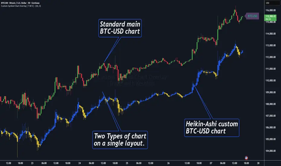
Custom Symbol Chart Overlay [ T W K ] :Custom Symbol Chart Overlay indicator for all types of Trading View account Users ❗
This Indicator has specially designed for apply Custom Symbol / Script on chart, in addition to current Live Chart symbol.
**No need for separate chart layout ( available for Paid Trading View users only! )
▫️▷ : # Indicator have settings for fetch the different Chart types (ex - Heikin-Ashi / standard) data and have the input for this.
all you need is to just select the Chart type. This setting allows user to apply different types of chart on single layout screen.
✔ (ex 1:- Standard current chart of BTCUSD ( SPOT ) with Custom Heikin-Ashi chart of BTCUSD ( PERPETUAL futures ).
✔ (ex 2:- Standard current chart of XAUUSD ( CFDs ) with Custom Standard chart of XAUUSD ( CFDs ) with MA / BB / ST input.
▫️▷ : It has 3 Moving average Lines, Bollinger Bands, and Super Trend input. (*Note:- all Inputs are customizable)
▫️▷ : # Indicator have ⏰ Alerts for automation trading ( #algo ) : Super Trend (3 conditions)
Usage:- This Indicator is helpful for apply Multiple symbols of different chart types on single layout screen.
Compatible with All Devices (Laptop / Mobile / Tablet / PC).
✅ HOW TO GET ACCESS :
Add to favorite and enjoy the true Trading View's sprit of community growth, without any limitations.
🔆If you like any of my Invite-Only indicators , kindly DM and let me know!
⚠ RISK DISCLAIMER :
All content provided by "@TradeWithKeshhav" is for informational & educational purposes only.
It does not constitute any financial advice or a solicitation to buy or sell any securities of any type. All investments / trading involve risks. Past performance does not guarantee future results / returns.
Regards :
Team @TradeWithKeshhav
Happy trading and investing!
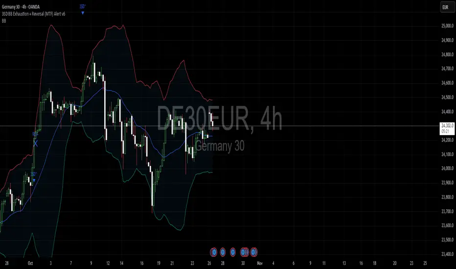
3SD Bollinger Exhaustion & Reversal Alert IndicatorThe Bollinger Band 3 Standard Deviation (3SD) captures roughly 99% of price action within its boundaries.
When price moves beyond these extremes, it often signals temporary overextension — creating opportunities for mean reversion trades, especially when aligned with the prevailing trend.
This indicator alerts you when:
- Price touches the 3SD Bollinger Band on higher timeframes (H4, D1, W1, M1), and
- A reversal reaction occurs — defined by a bullish or bearish candle close on H1 or H4.
Together, these conditions identify potential high-probability entry zones where exhaustion meets trend alignment.
🚀 Coming Soon
A premium version is in development, combining this 3SD exhaustion logic with my proprietary trend-following system.
It will generate confluence-based trade signals when price interacts with both the 3SD band and the trend-following band.
Stay tuned for updates.
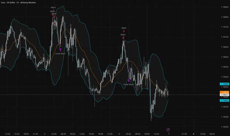
RSI Reversal + BB RSIReversal Alerts
SELL Reversal (reversalSELL)
Triggers when:
RSI touches or crosses above the upper BB, and
The current candle is bearish (close < open).
→ Plots a small red circle above the candle
→ Fires alert named “reversalSELL”
BUY Reversal (reversalBUY)
Triggers when:
RSI touches or crosses below the lower BB, and
The current candle is bullish (close > open).
→ Plots a small green circle below the candle
→ Fires alert named “reversalBUY”

Bollinger Band ToolkitBollinger Band Toolkit
An advanced, adaptive Bollinger Band system for traders who want more context, precision, and edge.
This indicator expands on the classic Bollinger Bands by combining statistical and volatility-based methods with modern divergence and squeeze detection tools. It helps identify volatility regimes, potential breakouts, and early momentum shifts — all within one clean overlay.
🔹 Core Features
1. Adaptive Bollinger Bands (σ + ATR)
Classic 20-period bands enhanced with an ATR-based volatility adjustment, making them more responsive to true market movement rather than just price variance.
Reduces “overreacting” during chop and avoids bands collapsing too tightly during trends.
2. %B & RSI Divergence Detection
🟢 Green dots: Positive %B divergence — price makes a lower low, but %B doesn’t confirm (bullish).
🔴 Red dots: Negative %B divergence — price makes a higher high, but %B doesn’t confirm (bearish).
✚ Red/green crosses: RSI divergence confirmation — momentum fails to confirm the price’s new extreme.
These signals highlight potential reversal or slowdown zones that are often invisible to the naked eye.
3. Bollinger Band Squeeze (with Volume Filter)
Yellow squares (■) show periods when Bollinger Bands are at their narrowest relative to recent history.
Volume confirmation ensures the squeeze only triggers when both volatility and participation contract.
Often marks the “calm before the storm” — breakout potential zones.
4. Multi-Timeframe Breakout Markers
Optionally displays breakouts from higher or lower timeframes using different colors/symbols.
Lets you see when a higher timeframe band break aligns with your current chart — a strong trend continuation signal.
5. Dual- and Triple-Band Visualization (±1σ, ±2σ, ±3σ)
Optional inner (±1σ) and outer (±3σ) bands provide a layered volatility map:
Price holding between ±1σ → stable range / mean-reverting behavior
Price riding near ±2σ → trending phase, sustained momentum
Price touching or exceeding ±3σ → volatility expansion or exhaustion zone
This triple-band layout visually distinguishes normal movement from statistical extremes, helping you read when the market is balanced, expanding, or approaching its limits.
⚙️ Inputs & Customization
Choose band type (SMA/EMA/SMMA/WMA/VWMA)
Adjust deviation multiplier (σ) and ATR multiplier
Toggle individual features (divergence dots, squeeze markers, inner bands, etc.)
Multi-timeframe and colour controls for advanced users
🧠 How to Use
Watch for squeeze markers followed by a breakout bar beyond ±2σ → volatility expansion signal.
Combine divergence dots with RSI or price structure to anticipate slowdowns or reversals.
Confirm direction using multi-timeframe breakouts and volume expansion.
💬 Why It Works
This toolkit transforms qualitative chart reading (tight bands, hidden divergence) into quantitative, testable conditions — giving you objective insights that can be backtested, coded, or simply trusted in live setups.

Copeland Dynamic Dominance Matrix System | GForgeCopeland Dynamic Dominance Matrix System | GForge - v1
---
📊 COMPREHENSIVE SYSTEM OVERVIEW
The GForge Dynamic BB% TrendSync System represents a revolutionary approach to algorithmic portfolio management, combining cutting-edge statistical analysis, momentum detection, and regime identification into a unified framework. This system processes up to 39 different cryptocurrency assets simultaneously, using advanced mathematical models to determine optimal capital allocation across dynamic market conditions.
Core Innovation: Multi-Dimensional Analysis
Unlike traditional single-asset indicators, this system operates on multiple analytical dimensions:
Momentum Analysis: Dual Bollinger Band Modified Deviation (DBBMD) calculations
Relative Strength: Comprehensive dominance matrix with head-to-head comparisons
Fundamental Screening: Alpha and Beta statistical filtering
Market Regime Detection: Five-component statistical testing framework
Portfolio Optimization: Dynamic weighting and allocation algorithms
Risk Management: Multi-layered protection and regime-based positioning
---
🔧 DETAILED COMPONENT BREAKDOWN
1. Dynamic Bollinger Band % Modified Deviation Engine (DBBMD)
The foundation of this system is an advanced oscillator that combines two independent Bollinger Band systems with asymmetric parameters to create unique momentum readings.
Technical Implementation:
[
// BB System 1: Fast-reacting with extended standard deviation
primary_bb1_ma_len = 40 // Shorter MA for responsiveness
primary_bb1_sd_len = 65 // Longer SD for stability
primary_bb1_mult = 1.0 // Standard deviation multiplier
// BB System 2: Complementary asymmetric design
primary_bb2_ma_len = 8 // Longer MA for trend following
primary_bb2_sd_len = 66 // Shorter SD for volatility sensitivity
primary_bb2_mult = 1.7 // Wider bands for reduced noise
Key Features:
Asymmetric Design: The intentional mismatch between MA and Standard Deviation periods creates unique oscillation characteristics that traditional Bollinger Bands cannot achieve
Percentage Scale: All readings are normalized to 0-100% scale for consistent interpretation across assets
Multiple Combination Modes:
BB1 Only: Fast/reactive system
BB2 Only: Smooth/stable system
Average: Balanced blend (recommended)
Both Required: Conservative (both must agree)
Either One: Aggressive (either can trigger)
Mean Deviation Filter: Additional volatility-based layer that measures the standard deviation of the DBBMD% itself, creating dynamic trigger bands
Signal Generation Logic:
// Primary thresholds
primary_long_threshold = 71 // DBBMD% level for bullish signals
primary_short_threshold = 33 // DBBMD% level for bearish signals
// Mean Deviation creates dynamic bands around these thresholds
upper_md_band = combined_bb + (md_mult * bb_std)
lower_md_band = combined_bb - (md_mult * bb_std)
// Signal triggers when DBBMD crosses these dynamic bands
long_signal = lower_md_band > long_threshold
short_signal = upper_md_band < short_threshold
For more information on this BB% indicator, find it here:
2. Revolutionary Dominance Matrix System
This is the system's most sophisticated innovation - a comprehensive framework that compares every asset against every other asset to determine relative strength hierarchies.
Mathematical Foundation:
The system constructs a mathematical matrix where each cell represents whether asset i dominates asset j:
// Core dominance matrix (39x39 for maximum assets)
var matrix dominance_matrix = matrix.new(39, 39, 0)
// For each qualifying asset pair (i,j):
for i = 0 to active_count - 1
for j = 0 to active_count - 1
if i != j
// Calculate price ratio BB% TrendSync for asset_i/asset_j
ratio_array = calculate_price_ratios(asset_i, asset_j)
ratio_dbbmd = calculate_dbbmd(ratio_array)
// Asset i dominates j if ratio is in uptrend
if ratio_dbbmd_state == 1
matrix.set(dominance_matrix, i, j, 1)
Copeland Scoring Algorithm:
Each asset receives a dominance score calculated as:
Dominance Score = Total Wins - Total Losses
// Calculate net dominance for each asset
for i = 0 to active_count - 1
wins = 0
losses = 0
for j = 0 to active_count - 1
if i != j
if matrix.get(dominance_matrix, i, j) == 1
wins += 1
else
losses += 1
copeland_score = wins - losses
array.set(dominance_scores, i, copeland_score)
Head-to-Head Analysis Process:
Ratio Construction: For each asset pair, calculate price_asset_A / price_asset_B
DBBMD Application: Apply the same DBBMD analysis to these ratios
Trend Determination: If ratio DBBMD shows uptrend, Asset A dominates Asset B
Matrix Population: Store dominance relationships in mathematical matrix
Score Calculation: Sum wins minus losses for final ranking
This creates a tournament-style ranking where each asset's strength is measured against all others, not just against a benchmark.
3. Advanced Alpha & Beta Filtering System
The system incorporates fundamental analysis through Capital Asset Pricing Model (CAPM) calculations to filter assets based on risk-adjusted performance.
Alpha Calculation (Excess Return Analysis):
// CAPM Alpha calculation
f_calc_alpha(asset_prices, benchmark_prices, alpha_length, beta_length, risk_free_rate) =>
// Calculate asset and benchmark returns
asset_returns = calculate_returns(asset_prices, alpha_length)
benchmark_returns = calculate_returns(benchmark_prices, alpha_length)
// Get beta for expected return calculation
beta = f_calc_beta(asset_prices, benchmark_prices, beta_length)
// Average returns over period
avg_asset_return = array_average(asset_returns) * 100
avg_benchmark_return = array_average(benchmark_returns) * 100
// Expected return using CAPM: E(R) = Beta * Market_Return + Risk_Free_Rate
expected_return = beta * avg_benchmark_return + risk_free_rate
// Alpha = Actual Return - Expected Return
alpha = avg_asset_return - expected_return
Beta Calculation (Volatility Relationship):
// Beta measures how much an asset moves relative to benchmark
f_calc_beta(asset_prices, benchmark_prices, length) =>
// Calculate return series for both assets
asset_returns =
benchmark_returns =
// Populate return arrays
for i = 0 to length - 1
asset_return = (current_price - previous_price) / previous_price
benchmark_return = (current_bench - previous_bench) / previous_bench
// Calculate covariance and variance
covariance = calculate_covariance(asset_returns, benchmark_returns)
benchmark_variance = calculate_variance(benchmark_returns)
// Beta = Covariance(Asset, Market) / Variance(Market)
beta = covariance / benchmark_variance
Filtering Applications:
Alpha Filter: Only includes assets with alpha above specified threshold (e.g., >0.5% monthly excess return)
Beta Filter: Screens for desired volatility characteristics (e.g., beta >1.0 for aggressive assets)
Combined Screening: Both filters must pass for asset qualification
Dynamic Thresholds: User-configurable parameters for different market conditions
4. Intelligent Tie-Breaking Resolution System
When multiple assets have identical dominance scores, the system employs sophisticated methods to determine final rankings.
Standard Tie-Breaking Hierarchy:
// Primary tie-breaking logic
if score_i == score_j // Tied dominance scores
// Level 1: Compare Beta values (higher beta wins)
beta_i = array.get(beta_values, i)
beta_j = array.get(beta_values, j)
if beta_j > beta_i
swap_positions(i, j)
else if beta_j == beta_i
// Level 2: Compare Alpha values (higher alpha wins)
alpha_i = array.get(alpha_values, i)
alpha_j = array.get(alpha_values, j)
if alpha_j > alpha_i
swap_positions(i, j)
Advanced Tie-Breaking (Head-to-Head Analysis):
For the top 3 performers, an enhanced tie-breaking mechanism analyzes direct head-to-head price ratio performance:
// Advanced tie-breaker for top performers
f_advanced_tiebreaker(asset1_idx, asset2_idx, lookback_period) =>
// Calculate price ratio over lookback period
ratio_history =
for k = 0 to lookback_period - 1
price_ratio = price_asset1 / price_asset2
array.push(ratio_history, price_ratio)
// Apply simplified trend analysis to ratio
current_ratio = array.get(ratio_history, 0)
average_ratio = calculate_average(ratio_history)
// Asset 1 wins if current ratio > average (trending up)
if current_ratio > average_ratio
return 1 // Asset 1 dominates
else
return -1 // Asset 2 dominates
5. Five-Component Aggregate Market Regime Filter
This sophisticated framework combines multiple statistical tests to determine whether market conditions favor trending strategies or require defensive positioning.
Component 1: Augmented Dickey-Fuller (ADF) Test
Tests for unit root presence to distinguish between trending and mean-reverting price series.
// Simplified ADF implementation
calculate_adf_statistic(price_series, lookback) =>
// Calculate first differences
differences =
for i = 0 to lookback - 2
diff = price_series - price_series
array.push(differences, diff)
// Statistical analysis of differences
mean_diff = calculate_mean(differences)
std_diff = calculate_standard_deviation(differences)
// ADF statistic approximation
adf_stat = mean_diff / std_diff
// Compare against threshold for trend determination
is_trending = adf_stat <= adf_threshold
Component 2: Directional Movement Index (DMI)
Classic Wilder indicator measuring trend strength through directional movement analysis.
// DMI calculation for trend strength
calculate_dmi_signal(high_data, low_data, close_data, period) =>
// Calculate directional movements
plus_dm_sum = 0.0
minus_dm_sum = 0.0
true_range_sum = 0.0
for i = 1 to period
// Directional movements
up_move = high_data - high_data
down_move = low_data - low_data
// Accumulate positive/negative movements
if up_move > down_move and up_move > 0
plus_dm_sum += up_move
if down_move > up_move and down_move > 0
minus_dm_sum += down_move
// True range calculation
true_range_sum += calculate_true_range(i)
// Calculate directional indicators
di_plus = 100 * plus_dm_sum / true_range_sum
di_minus = 100 * minus_dm_sum / true_range_sum
// ADX calculation
dx = 100 * math.abs(di_plus - di_minus) / (di_plus + di_minus)
adx = dx // Simplified for demonstration
// Trending if ADX above threshold
is_trending = adx > dmi_threshold
Component 3: KPSS Stationarity Test
Complementary test to ADF that examines stationarity around trend components.
// KPSS test implementation
calculate_kpss_statistic(price_series, lookback, significance_level) =>
// Calculate mean and variance
series_mean = calculate_mean(price_series, lookback)
series_variance = calculate_variance(price_series, lookback)
// Cumulative sum of deviations
cumulative_sum = 0.0
cumsum_squared_sum = 0.0
for i = 0 to lookback - 1
deviation = price_series - series_mean
cumulative_sum += deviation
cumsum_squared_sum += math.pow(cumulative_sum, 2)
// KPSS statistic
kpss_stat = cumsum_squared_sum / (lookback * lookback * series_variance)
// Compare against critical values
critical_value = significance_level == 0.01 ? 0.739 :
significance_level == 0.05 ? 0.463 : 0.347
is_trending = kpss_stat >= critical_value
Component 4: Choppiness Index
Measures market directionality using fractal dimension analysis of price movement.
// Choppiness Index calculation
calculate_choppiness(price_data, period) =>
// Find highest and lowest over period
highest = price_data
lowest = price_data
true_range_sum = 0.0
for i = 0 to period - 1
if price_data > highest
highest := price_data
if price_data < lowest
lowest := price_data
// Accumulate true range
if i > 0
true_range = calculate_true_range(price_data, i)
true_range_sum += true_range
// Choppiness calculation
range_high_low = highest - lowest
choppiness = 100 * math.log10(true_range_sum / range_high_low) / math.log10(period)
// Trending if choppiness below threshold (typically 61.8)
is_trending = choppiness < 61.8
Component 5: Hilbert Transform Analysis
Phase-based cycle detection and trend identification using mathematical signal processing.
// Hilbert Transform trend detection
calculate_hilbert_signal(price_data, smoothing_period, filter_period) =>
// Smooth the price data
smoothed_price = calculate_moving_average(price_data, smoothing_period)
// Calculate instantaneous phase components
// Simplified implementation for demonstration
instant_phase = smoothed_price
delayed_phase = calculate_moving_average(price_data, filter_period)
// Compare instantaneous vs delayed signals
phase_difference = instant_phase - delayed_phase
// Trending if instantaneous leads delayed
is_trending = phase_difference > 0
Aggregate Regime Determination:
// Combine all five components
regime_calculation() =>
trending_count = 0
total_components = 0
// Test each enabled component
if enable_adf and adf_signal == 1
trending_count += 1
if enable_adf
total_components += 1
// Repeat for all five components...
// Calculate trending proportion
trending_proportion = trending_count / total_components
// Market is trending if proportion above threshold
regime_allows_trading = trending_proportion >= regime_threshold
The system only allows asset positions when the specified percentage of components indicate trending conditions. During choppy or mean-reverting periods, the system automatically positions in USD to preserve capital.
6. Dynamic Portfolio Weighting Framework
Six sophisticated allocation methodologies provide flexibility for different market conditions and risk preferences.
Weighting Method Implementations:
1. Equal Weight Distribution:
// Simple equal allocation
if weighting_mode == "Equal Weight"
weight_per_asset = 1.0 / selection_count
for i = 0 to selection_count - 1
array.push(weights, weight_per_asset)
2. Linear Dominance Scaling:
// Linear scaling based on dominance scores
if weighting_mode == "Linear Dominance"
// Normalize scores to 0-1 range
min_score = array.min(dominance_scores)
max_score = array.max(dominance_scores)
score_range = max_score - min_score
total_weight = 0.0
for i = 0 to selection_count - 1
score = array.get(dominance_scores, i)
normalized = (score - min_score) / score_range
weight = 1.0 + normalized * concentration_factor
array.push(weights, weight)
total_weight += weight
// Normalize to sum to 1.0
for i = 0 to selection_count - 1
current_weight = array.get(weights, i)
array.set(weights, i, current_weight / total_weight)
3. Conviction Score (Exponential):
// Exponential scaling for high conviction
if weighting_mode == "Conviction Score"
// Combine dominance score with DBBMD strength
conviction_scores =
for i = 0 to selection_count - 1
dominance = array.get(dominance_scores, i)
dbbmd_strength = array.get(dbbmd_values, i)
conviction = dominance + (dbbmd_strength - 50) / 25
array.push(conviction_scores, conviction)
// Exponential weighting
total_weight = 0.0
for i = 0 to selection_count - 1
conviction = array.get(conviction_scores, i)
normalized = normalize_score(conviction)
weight = math.pow(1 + normalized, concentration_factor)
array.push(weights, weight)
total_weight += weight
// Final normalization
normalize_weights(weights, total_weight)
Advanced Features:
Minimum Position Constraint: Prevents dust allocations below specified threshold
Concentration Factor: Adjustable parameter controlling weight distribution aggressiveness
Dominance Boost: Extra weight for assets exceeding specified dominance thresholds
Dynamic Rebalancing: Automatic weight recalculation on portfolio changes
7. Intelligent USD Management System
The system treats USD as a competing asset with its own dominance score, enabling sophisticated cash management.
USD Scoring Methodologies:
Smart Competition Mode (Recommended):
f_calculate_smart_usd_dominance() =>
usd_wins = 0
// USD beats assets in downtrends or weak uptrends
for i = 0 to active_count - 1
asset_state = get_asset_state(i)
asset_dbbmd = get_asset_dbbmd(i)
// USD dominates shorts and weak longs
if asset_state == -1 or (asset_state == 1 and asset_dbbmd < long_threshold)
usd_wins += 1
// Calculate Copeland-style score
base_score = usd_wins - (active_count - usd_wins)
// Boost during weak market conditions
qualified_assets = count_qualified_long_assets()
if qualified_assets <= active_count * 0.2
base_score := math.round(base_score * usd_boost_factor)
base_score
Auto Short Count Mode:
// USD dominance based on number of bearish assets
usd_dominance = count_assets_in_short_state()
// Apply boost during low activity
if qualified_long_count <= active_count * 0.2
usd_dominance := usd_dominance * usd_boost_factor
Regime-Based USD Positioning:
When the five-component regime filter indicates unfavorable conditions, the system automatically overrides all asset signals and positions 100% in USD, protecting capital during choppy markets.
8. Multi-Asset Infrastructure & Data Management
The system maintains comprehensive data structures for up to 39 assets simultaneously.
Data Collection Framework:
// Full OHLC data matrices (200 bars depth for performance)
var matrix open_data = matrix.new(39, 200, na)
var matrix high_data = matrix.new(39, 200, na)
var matrix low_data = matrix.new(39, 200, na)
var matrix close_data = matrix.new(39, 200, na)
// Real-time data collection
if barstate.isconfirmed
for i = 0 to active_count - 1
ticker = array.get(assets, i)
= request.security(ticker, timeframe.period,
[open , high , low , close ],
lookahead=barmerge.lookahead_off)
// Store in matrices with proper shifting
matrix.set(open_data, i, 0, nz(o, 0))
matrix.set(high_data, i, 0, nz(h, 0))
matrix.set(low_data, i, 0, nz(l, 0))
matrix.set(close_data, i, 0, nz(c, 0))
Asset Configuration:
The system comes pre-configured with 39 major cryptocurrency pairs across multiple exchanges:
Major Pairs: BTC, ETH, XRP, SOL, DOGE, ADA, etc.
Exchange Coverage: Binance, KuCoin, MEXC for optimal liquidity
Configurable Count: Users can activate 2-39 assets based on preferences
Custom Tickers: All asset selections are user-modifiable
---
⚙️ COMPREHENSIVE CONFIGURATION GUIDE
Portfolio Management Settings
Maximum Portfolio Size (1-10):
Conservative (1-2): High concentration, captures strong trends
Balanced (3-5): Moderate diversification with trend focus
Diversified (6-10): Lower concentration, broader market exposure
Dominance Clarity Threshold (0.1-1.0):
Low (0.1-0.4): Prefers diversification, holds multiple assets frequently
Medium (0.5-0.7): Balanced approach, context-dependent allocation
High (0.8-1.0): Concentration-focused, single asset preference
Signal Generation Parameters
DBBMD Thresholds:
// Standard configuration
primary_long_threshold = 71 // Conservative: 75+, Aggressive: 65-70
primary_short_threshold = 33 // Conservative: 25-30, Aggressive: 35-40
// BB System parameters
bb1_ma_len = 40 // Fast system: 20-50
bb1_sd_len = 65 // Stability: 50-80
bb2_ma_len = 8 // Trend: 60-100
bb2_sd_len = 66 // Sensitivity: 10-20
Risk Management Configuration
Alpha/Beta Filters:
Alpha Threshold: 0.0-2.0% (higher = more selective)
Beta Threshold: 0.5-2.0 (1.0+ for aggressive assets)
Calculation Periods: 20-50 bars (longer = more stable)
Regime Filter Settings:
Trending Threshold: 0.3-0.8 (higher = stricter trend requirements)
Component Lookbacks: 30-100 bars (balance responsiveness vs stability)
Enable/Disable: Individual component control for customization
---
📊 PERFORMANCE TRACKING & VISUALIZATION
Real-Time Dashboard Features
The compact dashboard provides essential information:
Current Holdings: Asset names and allocation percentages
Dominance Score: Current position's relative strength ranking
Active Assets: Qualified long signals vs total asset count
Returns: Total portfolio performance percentage
Maximum Drawdown: Peak-to-trough decline measurement
Trade Count: Total portfolio transitions executed
Regime Status: Current market condition assessment
Comprehensive Ranking Table
The left-side table displays detailed asset analysis:
Ranking Position: Numerical order by dominance score
Asset Symbol: Clean ticker identification with color coding
Dominance Score: Net wins minus losses in head-to-head comparisons
Win-Loss Record: Detailed breakdown of dominance relationships
DBBMD Reading: Current momentum percentage with threshold highlighting
Alpha/Beta Values: Fundamental analysis metrics when filters enabled
Portfolio Weight: Current allocation percentage in signal portfolio
Execution Status: Visual indicator of actual holdings vs signals
Visual Enhancement Features
Color-Coded Assets: 39 distinct colors for easy identification
Regime Background: Red tinting during unfavorable market conditions
Dynamic Equity Curve: Portfolio value plotted with position-based coloring
Status Indicators: Symbols showing execution vs signal states
---
🔍 ADVANCED TECHNICAL FEATURES
State Persistence System
The system maintains asset states across bars to prevent excessive switching:
// State tracking for each asset and ratio combination
var array asset_states = array.new(1560, 0) // 39 * 40 ratios
// State changes only occur on confirmed threshold breaks
if long_crossover and current_state != 1
current_state := 1
array.set(asset_states, asset_index, 1)
else if short_crossover and current_state != -1
current_state := -1
array.set(asset_states, asset_index, -1)
Transaction Cost Integration
Realistic modeling of trading expenses:
// Transaction cost calculation
transaction_fee = 0.4 // Default 0.4% (fees + slippage)
// Applied on portfolio transitions
if should_execute_transition
was_holding_assets = check_current_holdings()
will_hold_assets = check_new_signals()
// Charge fees for meaningful transitions
if transaction_fee > 0 and (was_holding_assets or will_hold_assets)
fee_amount = equity * (transaction_fee / 100)
equity -= fee_amount
total_fees += fee_amount
Dynamic Memory Management
Optimized data structures for performance:
200-Bar History: Sufficient for calculations while maintaining speed
Matrix Operations: Efficient storage and retrieval of multi-asset data
Array Recycling: Memory-conscious data handling for long-running backtests
Conditional Calculations: Skip unnecessary computations during initialization
12H 30 assets portfolio
---
🚨 SYSTEM LIMITATIONS & TESTING STATUS
CURRENT DEVELOPMENT PHASE: ACTIVE TESTING & OPTIMIZATION
This system represents cutting-edge algorithmic trading technology but remains in continuous development. Key considerations:
Known Limitations:
Requires significant computational resources for 39-asset analysis
Performance varies significantly across different market conditions
Complex parameter interactions may require extensive optimization
Slippage and liquidity constraints not fully modeled for all assets
No consideration for market impact in large position sizes
Areas Under Active Development:
Enhanced regime detection algorithms
Improved transaction cost modeling
Additional portfolio weighting methodologies
Machine learning integration for parameter optimization
Cross-timeframe analysis capabilities
---
🔒 ANTI-REPAINTING ARCHITECTURE & LIVE TRADING READINESS
One of the most critical aspects of any trading system is ensuring that signals and calculations are based on confirmed, historical data rather than current bar information that can change throughout the trading session. This system implements comprehensive anti-repainting measures to ensure 100% reliability for live trading .
The Repainting Problem in Trading Systems
Repainting occurs when an indicator uses current, unconfirmed bar data in its calculations, causing:
False Historical Signals: Backtests appear better than reality because calculations change as bars develop
Live Trading Failures: Signals that looked profitable in testing fail when deployed in real markets
Inconsistent Results: Different results when running the same indicator at different times during a trading session
Misleading Performance: Inflated win rates and returns that cannot be replicated in practice
GForge Anti-Repainting Implementation
This system eliminates repainting through multiple technical safeguards:
1. Historical Data Usage for All Calculations
// CRITICAL: All calculations use PREVIOUS bar data (note the offset)
= request.security(ticker, timeframe.period,
[open , high , low , close , close],
lookahead=barmerge.lookahead_off)
// Store confirmed previous bar OHLC for calculations
matrix.set(open_data, i, 0, nz(o1, 0)) // Previous bar open
matrix.set(high_data, i, 0, nz(h1, 0)) // Previous bar high
matrix.set(low_data, i, 0, nz(l1, 0)) // Previous bar low
matrix.set(close_data, i, 0, nz(c1, 0)) // Previous bar close
// Current bar close only for visualization
matrix.set(current_prices, i, 0, nz(c0, 0)) // Live price display
2. Confirmed Bar State Processing
// Only process data when bars are confirmed and closed
if barstate.isconfirmed
// All signal generation and portfolio decisions occur here
// using only historical, unchanging data
// Shift historical data arrays
for i = 0 to active_count - 1
for bar = math.min(data_bars, 199) to 1
// Move confirmed data through historical matrices
old_data = matrix.get(close_data, i, bar - 1)
matrix.set(close_data, i, bar, old_data)
// Process new confirmed bar data
calculate_all_signals_and_dominance()
3. Lookahead Prevention
// Explicit lookahead prevention in all security calls
request.security(ticker, timeframe.period, expression,
lookahead=barmerge.lookahead_off)
// This ensures no future data can influence current calculations
// Essential for maintaining signal integrity across all timeframes
4. State Persistence with Historical Validation
// Asset states only change based on confirmed threshold breaks
// using historical data that cannot change
var array asset_states = array.new(1560, 0)
// State changes use only confirmed, previous bar calculations
if barstate.isconfirmed
=
f_calculate_enhanced_dbbmd(confirmed_price_array, ...)
// Only update states after bar confirmation
if long_crossover_confirmed and current_state != 1
current_state := 1
array.set(asset_states, asset_index, 1)
Live Trading vs. Backtesting Consistency
The system's architecture ensures identical behavior in both environments:
Backtesting Mode:
Uses historical offset data for all calculations
Processes confirmed bars with `barstate.isconfirmed`
Maintains identical signal generation logic
No access to future information
Live Trading Mode:
Uses same historical offset data structure
Waits for bar confirmation before signal updates
Identical mathematical calculations and thresholds
Real-time price display without affecting signals
Technical Implementation Details
Data Collection Timing
// Example of proper data collection timing
if barstate.isconfirmed // Wait for bar to close
// Collect PREVIOUS bar's confirmed OHLC data
for i = 0 to active_count - 1
ticker = array.get(assets, i)
// Get confirmed previous bar data (note offset)
=
request.security(ticker, timeframe.period,
[open , high , low , close , close],
lookahead=barmerge.lookahead_off)
// ALL calculations use prev_* values
// current_close only for real-time display
portfolio_calculations_use_previous_bar_data()
Signal Generation Process
// Signal generation workflow (simplified)
if barstate.isconfirmed and data_bars >= minimum_required_bars
// Step 1: Calculate DBBMD using historical price arrays
for i = 0 to active_count - 1
historical_prices = get_confirmed_price_history(i) // Uses offset data
= calculate_dbbmd(historical_prices)
update_asset_state(i, state)
// Step 2: Build dominance matrix using confirmed data
calculate_dominance_relationships() // All historical data
// Step 3: Generate portfolio signals
new_portfolio = generate_target_portfolio() // Based on confirmed calculations
// Step 4: Compare with previous signals for changes
if portfolio_signals_changed()
execute_portfolio_transition()
Verification Methods for Users
Users can verify the anti-repainting behavior through several methods:
1. Historical Replay Test
Run the indicator on historical data
Note signal timing and portfolio changes
Replay the same period - signals should be identical
No retroactive changes in historical signals
2. Intraday Consistency Check
Load indicator during active trading session
Observe that previous day's signals remain unchanged
Only current day's final bar should show potential signal changes
Refresh indicator - historical signals should be identical
Live Trading Deployment Considerations
Data Quality Assurance
Exchange Connectivity: Ensure reliable data feeds for all 39 assets
Missing Data Handling: System includes safeguards for data gaps
Price Validation: Automatic filtering of obvious price errors
Timeframe Synchronization: All assets synchronized to same bar timing
Performance Impact of Anti-Repainting Measures
The robust anti-repainting implementation requires additional computational resources:
Memory Usage: 200-bar historical data storage for 39 assets
Processing Delay: Signals update only after bar confirmation
Calculation Overhead: Multiple historical data validations
Alert Timing: Slight delay compared to current-bar indicators
However, these trade-offs are essential for reliable live trading performance and accurate backtesting results.
Critical: Equity Curve Anti-Repainting Architecture
The most sophisticated aspect of this system's anti-repainting design is the temporal separation between signal generation and performance calculation . This creates a realistic trading simulation that perfectly matches live trading execution.
The Timing Sequence
// STEP 1: Store what we HELD during the current bar (for performance calc)
if barstate.isconfirmed
// Record positions that were active during this bar
array.clear(held_portfolio)
array.clear(held_weights)
for i = 0 to array.size(execution_portfolio) - 1
array.push(held_portfolio, array.get(execution_portfolio, i))
array.push(held_weights, array.get(execution_weights, i))
// STEP 2: Calculate performance based on what we HELD
portfolio_return = 0.0
for i = 0 to array.size(held_portfolio) - 1
held_asset = array.get(held_portfolio, i)
held_weight = array.get(held_weights, i)
// Performance from current_price vs reference_price
// This is what we ACTUALLY earned during this bar
if held_asset != "USD"
current_price = get_current_price(held_asset) // End of bar
reference_price = get_reference_price(held_asset) // Start of bar
asset_return = (current_price - reference_price) / reference_price
portfolio_return += asset_return * held_weight
// STEP 3: Apply return to equity (realistic timing)
equity := equity * (1 + portfolio_return)
// STEP 4: Generate NEW signals for NEXT period (using confirmed data)
= f_generate_target_portfolio()
// STEP 5: Execute transitions if signals changed
if signal_changed
// Update execution_portfolio for NEXT bar
array.clear(execution_portfolio)
array.clear(execution_weights)
for i = 0 to array.size(new_signal_portfolio) - 1
array.push(execution_portfolio, array.get(new_signal_portfolio, i))
array.push(execution_weights, array.get(new_signal_weights, i))
Why This Prevents Equity Curve Repainting
Performance Attribution: Returns are calculated based on positions that were **actually held** during each bar, not future signals
Signal Timing: New signals are generated **after** performance calculation, affecting only **future** bars
Realistic Execution: Mimics real trading where you earn returns on current positions while planning future moves
No Retroactive Changes: Once a bar closes, its performance contribution to equity is permanent and unchangeable
The One-Bar Offset Mechanism
This system implements a critical one-bar timing offset:
// Bar N: Performance Calculation
// ================================
// 1. Calculate returns on positions held during Bar N
// 2. Update equity based on actual holdings during Bar N
// 3. Plot equity point for Bar N (based on what we HELD)
// Bar N: Signal Generation
// ========================
// 4. Generate signals for Bar N+1 (using confirmed Bar N data)
// 5. Send alerts for what will be held during Bar N+1
// 6. Update execution_portfolio for Bar N+1
// Bar N+1: The Cycle Continues
// =============================
// 1. Performance calculated on positions from Bar N signals
// 2. New signals generated for Bar N+2
Alert System Timing
The alert system reflects this sophisticated timing:
Transaction Cost Realism
Even transaction costs follow realistic timing:
// Fees applied when transitioning between different portfolios
if should_execute_transition
// Charge fees BEFORE taking new positions (realistic timing)
if transaction_fee > 0
fee_amount = equity * (transaction_fee / 100)
equity -= fee_amount // Immediate cost impact
total_fees += fee_amount
// THEN update to new portfolio
update_execution_portfolio(new_signals)
transitions += 1
// Fees reduce equity immediately, affecting all future calculations
// This matches real trading where fees are deducted upon execution
LIVE TRADING CERTIFICATION:
This system has been specifically designed and tested for live trading deployment. The comprehensive anti-repainting measures ensure that:
Backtesting results accurately represent real trading potential
Signals are generated using only confirmed, historical data
No retroactive changes can occur to previously generated signals
Portfolio transitions are based on reliable, unchanging calculations
Performance metrics reflect realistic trading outcomes including proper timing
Users can deploy this system with confidence that live trading results will closely match backtesting performance, subject to normal market execution factors such as slippage and liquidity.
---
⚡ ALERT SYSTEM & AUTOMATION
The system provides comprehensive alerting for automation and monitoring:
Available Alert Conditions
Portfolio Signal Change: Triggered when new portfolio composition is generated
Regime Override Active: Alerts when market regime forces USD positioning
Individual Asset Signals: Can be configured for specific asset transitions
Performance Thresholds: Drawdown or return-based notifications
---
📈 BACKTESTING & PERFORMANCE ANALYSIS
8 Comprehensive Metrics Tracking
The system maintains detailed performance statistics:
Equity Curve: Real-time portfolio value progression
Returns Calculation: Total and annualized performance metrics
Drawdown Analysis: Peak-to-trough decline measurements
Transaction Counting: Portfolio transition frequency
Fee Tracking: Cumulative transaction cost impact
Win Rate Analysis: Success rate of position changes
Backtesting Configuration
// Backtesting parameters
initial_capital = 10000.0 // Starting capital
use_custom_start = true // Enable specific start date
custom_start = timestamp("2023-09-01") // Backtest beginning
transaction_fee = 0.4 // Combined fees and slippage %
// Performance calculation
total_return = (equity - initial_capital) / initial_capital * 100
current_drawdown = (peak_equity - equity) / peak_equity * 100
---
🔧 TROUBLESHOOTING & OPTIMIZATION
Common Configuration Issues
Insufficient Data: Ensure 100+ bars available before start date
[*} Not Compiling: Go on an asset's price chart with 2 or 3 years of data to
make the system compile or just simply reapply the indicator again
Too Many Assets: Reduce active count if experiencing timeouts
Regime Filter Too Strict: Lower trending threshold if always in USD
Excessive Switching: Increase MD multiplier or adjust thresholds
---
💡 USER FEEDBACK & ENHANCEMENT REQUESTS
The continuous evolution of this system depends heavily on user experience and community feedback. Your insights will help motivate me for new improvements and new feature developments.
---
⚖️ FINAL COMPREHENSIVE RISK DISCLAIMER
TRADING INVOLVES SUBSTANTIAL RISK OF LOSS
This indicator is a sophisticated analytical tool designed for educational and research purposes. Important warnings and considerations:
System Limitations:
No algorithmic system can guarantee profitable outcomes
Complex systems may fail in unexpected ways during extreme market events
Historical backtesting does not account for all real-world trading challenges
Slippage, liquidity constraints, and market impact can significantly affect results
System parameters require careful optimization and ongoing monitoring
The creator and distributor of this indicator assume no liability for any financial losses, system failures, or adverse outcomes resulting from its use. This tool is provided "as is" without any warranties, express or implied.
By using this indicator, you acknowledge that you have read, understood, and agreed to assume all risks associated with algorithmic trading and cryptocurrency investments.
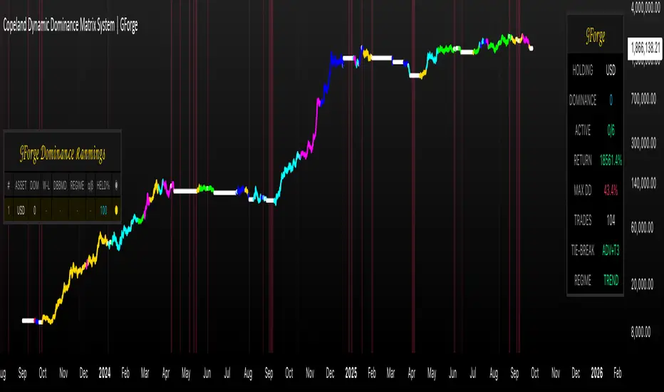
Hazel nut BB Strategy, volume base- lite versionHazel nut BB Strategy, volume base — lite version
Having knowledge and information in financial markets is only useful when a trader operates with a well-defined trading strategy. Trading strategies assist in capital management, profit-taking, and reducing potential losses.
This strategy is built upon the core principle of supply and demand dynamics. Alongside this foundation, one of the widely used technical tools — the Bollinger Bands — is employed to structure a framework for profit management and risk control.
In this strategy, the interaction of these tools is explained in detail. A key point to note is that for calculating buy and sell volumes, a lower timeframe function is used. When applied with a tick-level resolution, this provides the most precise measurement of buyer/seller flows. However, this comes with a limitation of reduced historical depth. Users should be aware of this trade-off: if precise tick-level data is required, shorter timeframes should be considered to extend historical coverage .
The strategy offers multiple configuration options. Nevertheless, it should be treated strictly as a supportive tool rather than a standalone trading system. Decisions must integrate personal analysis and other instruments. For example, in highly volatile assets with narrow ranges, it is recommended to adjust profit-taking and stop-loss percentages to smaller values.
◉ Volume Settings
• Buyer and seller volume (up/down volume) are requested from a lower timeframe, with an option to override the automatic resolution.
• A global lookback period is applied to calculate moving averages and cumulative sums of buy/sell/delta volumes.
• Ratios of buyers/sellers to total volume are derived both on the current bar and across the lookback window.
◉ Bollinger Band
• Bands are computed using configurable moving averages (SMA, EMA, RMA, WMA, VWMA).
• Inputs allow control of length, standard deviation multiplier, and offset.
• The basis, upper, and lower bands are plotted, with a shaded background between them.
◉ Progress & Proximity
• Relative position of the price to the Bollinger basis is expressed as percentages (qPlus/qMinus).
• “Near band” conditions are triggered when price progress toward the upper or lower band exceeds a user-defined threshold (%).
• A signed score (sScore) represents how far the close has moved above or below the basis relative to band width.
◉ Info Table
• Optional compact table summarizing:
• - Upper/lower band margins
• - Buyer/seller volumes with moving averages
• - Delta and cumulative delta
• - Buyer/seller ratios per bar and across the window
• - Money flow values (buy/sell/delta × price) for bar-level and summed periods
• The table is neutral-colored and resizable for different chart layouts.
◉ Zone Event Gate
• Tracks entry into and exit from “near band” zones.
• Arming logic: a side is armed when price enters a band proximity zone.
• Trigger logic: on exit, a trade event is generated if cumulative buyer or seller volume dominates over a configurable window.
◉ Trading Logic
• Orders are placed only on zone-exit events, conditional on volume dominance.
• Position sizing is defined as a fixed percentage of strategy equity.
• Long entries occur when leaving the lower zone with buyer dominance; short entries occur when leaving the upper zone with seller dominance.
◉ Exit Rules
• Open positions are managed by a strict priority sequence:
• 1. Stop-loss (% of entry price)
• 2. Take-profit (% of entry price)
• 3. Opposite-side event (zone exit with dominance in the other direction)
• Stop-loss and take-profit levels are configurable
◉ Notes
• This lite version is intended to demonstrate the interaction of Bollinger Bands and volume-based dominance logic.
• It provides a framework to observe how price reacts at band boundaries under varying buy/sell pressure, and how zone exits can be systematically converted into entry/exit signals.
When configuring this strategy, it is essential to carefully review the settings within the Strategy Tester. Ensure that the chosen parameters and historical data options are correctly aligned with the intended use. Accurate back testing depends on applying proper configurations for historical reference. The figure below illustrates sample result and configuration type.

Multi-Timeframe Bollinger BandsMy hope is to optimize the settings for this indicator and reintroduce it as a "strategy" with suggested position entry and exit points shown in the price pane.
I’ve been having good results setting the “Bollinger Band MA Length” in the Input tab to between 5 and 10. You can use the standard 20 period, but your results will not be as granular.
This indicator has proven very good at finding local tops and bottoms by combining data from multiple timeframes. Use timeframes that are lower than the timeframe you are viewing in your price pane. Be cognizant that the indicator, like other oscillators, does occasionally produce divergences at tops and bottoms.
Any feedback is appreciated.
Overview
This indicator is an oscillator that measures the normalized position of the price relative to Bollinger Bands across multiple timeframes. It takes the price's position within the Bollinger Bands (calculated on different timeframes) and averages those positions to create a single value that oscillates between 0 and 1. This value is then plotted as the oscillator, with reference lines and colored regions to help interpret the price's relative strength or weakness.
How It Works
Bollinger Band Calculation:
The indicator uses a custom function f_getBBPosition() to calculate the position of the price within Bollinger Bands for a given timeframe.
Price Position Normalization:
For each timeframe, the function normalizes the price's position between the upper and lower Bollinger Bands.
It calculates three positions based on the high, low, and close prices of the requested timeframe:
pos_high = (High - Lower Band) / (Upper Band - Lower Band)
pos_low = (Low - Lower Band) / (Upper Band - Lower Band)
pos_close = (Close - Lower Band) / (Upper Band - Lower Band)
If the upper band is not greater than the lower band or if the data is invalid (e.g., na), it defaults to 0.5 (the midline).
The average of these three positions (avg_pos) represents the normalized position for that timeframe, ranging from 0 (at the lower band) to 1 (at the upper band).
Multi-Timeframe Averaging:
The indicator fetches Bollinger Band data from four customizable timeframes (default: 30min, 60min, 240min, daily) using request.security() with lookahead=barmerge.lookahead_on to get the latest available data.
It calculates the normalized position (pos1, pos2, pos3, pos4) for each timeframe using f_getBBPosition().
These four positions are then averaged to produce the final avg_position:avg_position = (pos1 + pos2 + pos3 + pos4) / 4
This average is the oscillator value, which is plotted and typically oscillates between 0 and 1.
Moving Averages:
Two optional moving averages (MA1 and MA2) of the avg_position can be enabled, calculated using simple moving averages (ta.sma) with customizable lengths (default: 5 and 10).
These can be potentially used for MA crossover strategies.
What Is Being Averaged?
The oscillator (avg_position) is the average of the normalized price positions within the Bollinger Bands across the four selected timeframes. Specifically:It averages the avg_pos values (pos1, pos2, pos3, pos4) calculated for each timeframe.
Each avg_pos is itself an average of the normalized positions of the high, low, and close prices relative to the Bollinger Bands for that timeframe.
This multi-timeframe averaging smooths out short-term fluctuations and provides a broader perspective on the price's position within the volatility bands.
Interpretation
0.0 The price is at or below the lower Bollinger Band across all timeframes (indicating potential oversold conditions).
0.15: A customizable level (green band) which can be used for exiting short positions or entering long positions.
0.5: The midline, where the price is at the average of the Bollinger Bands (neutral zone).
0.85: A customizable level (orange band) which can be used for exiting long positions or entering short positions.
1.0: The price is at or above the upper Bollinger Band across all timeframes (indicating potential overbought conditions).
The colored regions and moving averages (if enabled) help identify trends or crossovers for trading signals.
Example
If the 30min timeframe shows the close at the upper band (position = 1.0), the 60min at the midline (position = 0.5), the 240min at the lower band (position = 0.0), and the daily at the upper band (position = 1.0), the avg_position would be:(1.0 + 0.5 + 0.0 + 1.0) / 4 = 0.625
This value (0.625) would plot in the orange region (between 0.85 and 0.5), suggesting the price is relatively strong but not at an extreme.
Notes
The use of lookahead=barmerge.lookahead_on ensures the indicator uses the latest available data, making it more real-time, though its effectiveness depends on the chart timeframe and TradingView's data feed.
The indicator’s sensitivity can be adjusted by changing bb_length ("Bollinger Band MA Length" in the Input tab), bb_mult ("Bollinger Band Standard Deviation," also in the Input tab), or the selected timeframes.
Advanced VWAP Multi-MA System with Bollinger Bands & Dashboard📊 Key Features:
Core Functionality:
* VWAP Calculation with customizable anchor periods (Session/Week/Month/Quarter/Year)
* Multiple Moving Average Types (EMA, SMA, WMA, HMA, RMA, VWMA)
* Three MA Lengths (Fast: 9, Medium: 21, Slow: 50)
* Standard Deviation Bands with 3 levels (1σ, 2σ, 3σ)
* Dynamic band multipliers (adjustable from 0.5 to 5.0)
🎨 Visual Theme System:
* Theme Types: Dark, Light, Pro
* Visual Styles: Quantum, Holographic, Crystalline, Plasma, Nebula
* Visual Intensity Control (20-100%)
* Multi-layer Harmonic Nodes with gradient effects
* Energy Flow Lines based on momentum
* Minimal signal dots for buy/sell conditions
📈 Holographic Dashboard:
* Real-time VWAP position tracking
* MA trend analysis (Bullish/Bearish/Neutral)
* Band position indicator (±1σ, ±2σ, ±3σ)
* Volatility percentage
* Momentum direction
* Current visual theme display
✨ Visual Effects:
* Quantum Fields: Multi-layer boxes with dynamic transparency
* Energy Flow: Momentum-based directional lines
* Gradient Fills: Between bands and MAs
* Borderless Design: Clean, modern appearance
* Emoji Headers: Enhanced visual appeal (⚡ 🌌 📊 🔮)
🎯 Trading Signals:
* Bullish Signal: Close > VWAP AND Close > Fast MA AND Fast MA > Medium MA
* Bearish Signal: Close < VWAP AND Close < Fast MA AND Fast MA < Medium MA

CryptoPulseStoch AICryptoPulseStoch AI Strategy
This strategy combines Bollinger Bands, multi-timeframe EMAs (200 and 50), and Stochastic Oscillator for crypto trading signals on the 1-minute timeframe. Long entries trigger on Stochastic %K/%D crossovers in oversold zones with price breaking the lower Bollinger Band and an upward EMA trend; shorts on crossunders in overbought zones with price breaking the upper Bollinger Band and a downward EMA trend. Includes ATR-based risk management, position sizing, and R:R targets. Overlay on any chart; supports leverage (100% margin). Visual lines/labels for TP/SL/entries; alerts for webhooks.
- **Account Balance (Default: 10000)**: Initial balance for calculating risk and position size; increase for larger accounts.
- **BB Length (Default: 20)**: Periods for Bollinger Bands basis and deviation; shorter for more signals, longer for smoothing.
- **BB Multiplier (Default: 2.0)**: Std dev factor for band width; higher widens bands, reducing false breakouts.
- **Stochastic %K Length (Default: 14)**: Periods for Stochastic Oscillator %K calculation; adjust for sensitivity.
- **Stochastic Smooth K (Default: 1)**: Smoothing period for %K; higher values reduce noise.
- **Stochastic Smooth D (Default: 3)**: Smoothing period for %D; higher values smooth the signal line.
- **Overbought Level (Default: 70)**: Stochastic threshold for bearish signals; lower for more frequent signals.
- **Oversold Level (Default: 30)**: Stochastic threshold for bullish signals; higher for more frequent signals.
- **Risk Per Trade (%) (Default: 2.0)**: Account percentage risked per trade; lower for conservative sizing.
- **Risk:Reward Ratio (Default: 6.0)**: Target profit multiple of risk; higher aims for bigger wins.
- **SL Multiplier (Default: 9.0)**: ATR factor for stop loss distance; adjust based on volatility.
- **TP Multiplier (Default: 6.0)**: ATR factor for take profit distance, scaled by R:R; adjust for target distance.
- **Line Length (bars) (Default: 25)**: Bars to extend TP/SL/entry lines; longer for better visibility.
- **Label Position (Default: left)**: Text placement relative to lines (left/right); choose for chart clarity.
- **ATR Period (Default: 14)**: Periods for ATR volatility measure; affects SL, TP, and position size.
- **EMA Timeframe (Default: 5 min)**: Resolution for EMA 200/50 calculation; use lower TFs for finer trend confirmation.
- **Visuals**: BB plots (blue basis, green upper, red lower); EMA200 (red), EMA50 (green); Stochastic %K (blue), %D (orange); red/green lines/labels for sell/buy entries, SL (red), TP (green).
- **Alerts**: Conditions for buy/sell signals with webhook messages for integration (e.g., Bitget).

4H Bollinger Breakout StrategyThis strategy leverages Bollinger Bands on the 4-hour timeframe for long and short trades in trending or ranging markets. Entries trigger on BB breakouts with optional filters for volume, trend, and RSI. Exits occur on opposite BB crosses. Customizable for long-only, short-only, or indicator mode via code comments. Supports forex, stocks, or crypto with full equity allocation and 0.1% commission.
Length (Default: 20): Period for BB basis and std dev; shorter for sensitivity, longer for smoothing.
Basis MA Type (Default: SMA): Selects MA for middle band (SMA, EMA, etc.); EMA for faster response.
Source (Default: Close): Price input for calculations; use close for standard accuracy.
StdDev Multiplier (Default: 1.8): Band width control; higher for fewer signals, lower for more.
Offset (Default: 0): Shifts BB plots; typically unchanged.
Use Filters (Default: True): Applies volume, trend, RSI checks to filter signals.
Volume MA Length (Default: 20): For volume filter (long: >105% avg, short: >120%).
Trend MA Length (Default: 80): SMA for trend filter (long: above MA, short: below).
RSI Length (Default: 14): For short filter (entry if RSI <85).
Use Long/Short Signals (Defaults: True): Toggles directions; long entry on lower BB crossover, short on upper crossunder.
Visuals: BB plots (blue basis, red upper, green lower), orange trend MA, filled background.
Labels/Alerts: Green/red for long entry/exit, yellow/purple for short; alert conditions included.

Signalgo BBSignalgo BB: Technical Overview
Signalgo BB is a Bollinger Bands (BB) indicator for TradingView, designed to provide a multi-dimensional view of volatility, trend, and trading opportunities within a single overlay. Below is a detailed, impartial explanation of its workings, inputs, and trading logic.
Core Mechanics
Signalgo BB operates on the principle of nested volatility bands and moving averages. It calculates:
Fast & Slow Bands: Two sets of Bollinger Bands (BB), using different moving average types (EMA or SMA), lengths, and standard deviation multipliers.
Volatility Cloud: A dynamic visual layer indicating when price is inside both, one, or neither band.
Filtering: A short-term RSI is used to confirm trend direction and filter out weak signals.
Inputs & Components
MA Type: Choice between EMA, SMA for both fast and slow MA calculations.
Fast/Slow Lengths
Fast/Slow Deviations
RSI Length/Thresholds
Show Cloud: Toggle for the visual volatility cloud.
Signal Mode: Band Break.
Prevent Repeated Signals: Option to suppress duplicate signals in the same direction.
TP/SL & Trailing Logic: Advanced, automated trade management with ATR-based distances, three take-profit levels, and a dynamic trailing stop.
Signal Generation
Band Break: Triggers when price crosses the fast BB band.
RSI Filter: All signals require RSI confirmation.
Prevent Repeated Signals: Optionally only marks the first breakout in a series to reduce overtrading.
Entry/Exit Marks: Labels are plotted for visual clarity, and signals can trigger TradingView alerts.
Trade Management
Stop Loss (SL): Set at a multiple of ATR from the entry price, adapting to current volatility.
Take Profits (TP1, TP2, TP3): Three levels scaled by risk-reward ratios, supporting partial exits.
Trailing Stop: After the first TP is hit, SL moves to breakeven and then trails at a user-defined multiple of ATR, locking in further gains.
Event Markers: Each TP, SL, and trailing stop event is labeled on the chart.
Direction State: The indicator tracks active trades, allowing for only one open position per direction at a time.
Cloud Visualization: The background color changes depending on whether price is inside both, one, or no bands, making it easier to visualize market conditions.
Multiple Signal Logics: It doesn’t just look at breakouts, it includes cloud crossings, mean reversion, and a choice of how to combine them.
Rigorous Filtering: Signals require RSI trend confirmation, reducing false entries during weak phases.
Automated Trade Management: Built-in TP/SL and trailing logic, dynamically adapting to volatility.
Signal Suppression: Option to prevent repeated signals, reducing noise and overtrading.
Customizable MA Types: Supports EMA, SMA, and a selection algorithm for future expansion.
Trading Strategy Application
Volatility Regimes: The cloud’s color indicates whether price is inside, between, or outside the bands, helping traders identify trending, ranging, or breakout conditions.
Signals: entries can be based on breakouts filtered by RSI trend strength.
Risk Management: All active trades are managed by TP/SL logic, trailing stops after TP1, and visual feedback on exits.
Visual Alerts: Both signals and TP/SL events are marked on the chart for manual review.
Flexibility: Users can switch modes or suppress repeated signals as needed, depending on trading style.
Practical Usage
Intraday to Swing: Suitable for timeframes from minutes to days, depending on the MA periods and volatility profile.
Manual or Automated: The visual overlay and alerts support both manual trading and automated strategies.
Education & Review: The colored cloud and event markers make it easy to review past price action and learn from signals.
What separates this indicator from traditional ones:
1. Dual Bollinger Bands
Traditional: Most indicators use a single set of Bollinger Bands (two standard deviations above/below a moving average).
Signalgo BB: Implements two sets of bands—a "fast" set (shorter moving average, narrower deviation) and a "slow" set (longer moving average, wider deviation). This provides both immediate (fast) and broader context (slow) for volatility and price action.
2. Volatility Cloud Visualization
Traditional: Standard Bollinger Bands display as two lines, with the area between sometimes shaded as a "band" but without dynamic color changes.
Signalgo BB: The background is colored differently depending on whether price is within both, one, or neither band, offering a visual "cloud" that distinguishes trending, ranging, or breakout regimes at a glance.
3. RSI Filtering
Traditional: Many indicators either don’t filter signals, or if they do, it’s not always configurable.
Signalgo BB: Adds an optional RSI filter, requiring signals to be confirmed by short-term RSI overbought/oversold conditions. This reduces false signals in range-bound or low-trend environments.
4. Prevention of Repeated Signals
Traditional: Most indicators will keep firing signals as long as conditions are met, which can cause overtrading.
Signalgo BB: Offers a user-toggleable option to suppress repeated signals in the same direction until the opposite signal occurs. This reduces noise for discretionary traders.
5. Integrated Trade Management
Traditional: Manual or separate coding is required for stop-loss, take-profit, and trailing stop logic.
Signalgo BB: Builds in dynamic, ATR-based stop-loss; up to three take-profit levels and a trailing stop that activates after the first TP is hit. All levels are visually plotted on the chart, and events (TP/SL hits) are labeled, aiding strategy review and automation.
6. Event Labeling and Alerts
Traditional: Alerts may exist for entry/exit, but rarely for each TP/SL event.
Signalgo BB: Places labels for every entry, exit, and TP/SL event. It also provides TradingView alertconditions for each event, enabling automated notifications or integration with trading bots.
7. Directional State Tracking
Traditional: Indicators typically do not track the "state" of a trade (e.g., active long/short/flat) beyond simple signals.
Signalgo BB: Maintains persistent variables for entry price, SL, TP, trailing stop, and trade direction, ensuring only one active signal per direction. This prevents overlapping entries and mimics realistic trade management.
8. User Customization
Traditional: Default settings are often hardcoded, or customization is limited.
Signalgo BB: Offers extensive user inputs for MA type and TP/SL logic—making the tool adaptable to many strategies and timeframes.

Bollinger Band Breakout With Volatility StoplossDetailed Explanation of the Bollinger Band Breakout With Volatility Stoploss System
Introduction
The "Bollinger Band Breakout With Volatility Stoploss" system is a trading strategy designed to exploit price volatility in financial markets using the Bollinger Bands indicator, a widely recognized tool developed by John Bollinger. This system adapts the traditional Bollinger Bands framework into a Volatility Breakout strategy, focusing on capturing significant price movements by leveraging customized parameters and precise trading rules. The system operates exclusively on long positions, employs a daily timeframe, and incorporates dynamic risk management techniques to optimize trade outcomes while preserving capital.
System Parameters
The system modifies the standard Bollinger Bands configuration to suit its breakout methodology:
Standard Deviation (SD): Set to 1x, determining the width of the bands relative to the central moving average. This tighter setting enhances sensitivity to price movements, making the system responsive to smaller volatility shifts compared to the conventional 2x SD.
Period: A 30-day (1-month) lookback period is used to calculate the bands, providing a balance between capturing medium-term price trends and avoiding excessive noise from shorter timeframes.
Moving Average Type: The system uses an Exponential Moving Average (EMA) instead of the Simple Moving Average (SMA). The EMA places greater weight on recent price data, making it more responsive to current market conditions and better suited for detecting breakout opportunities in dynamic markets.
Core Concept
The Bollinger Band Breakout system is built on the principle of Volatility Breakout, which seeks to capitalize on significant price movements when the price breaks out of a defined volatility range. The Bollinger Bands, consisting of an EMA as the central line and two bands (Upper and Lower) calculated as the EMA plus or minus 1x SD, define this range. The system operates on a Daily Chart (D) timeframe, making it suitable for traders who prefer analyzing and executing trades based on daily price action. By focusing solely on Long Positions (buying low and selling high), the system avoids short-selling, aligning with strategies that capitalize on upward price momentum.
The core idea is to use the 1x SD multiplier over a 30-day period to establish a dynamic price range that reflects recent market volatility. Breakouts above the Upper Band signal potential buying opportunities, while penetrations below the Lower Band indicate exits, ensuring trades are aligned with significant price movements.
Trading Signals
The system generates clear entry and exit signals based on price interactions with the Bollinger Bands:
Buy Signal: A buy signal is triggered when the closing price of a daily candle exceeds the Upper Bollinger Band (EMA + 1x SD over 30 days). The trade is entered at the opening price of the subsequent candle, ensuring the breakout is confirmed by the close of the prior day. This approach minimizes false signals by waiting for a definitive breach of the volatility threshold.
Sell Signal: A sell signal occurs when the closing price falls below the Lower Bollinger Band (EMA - 1x SD over 30 days). The position is exited at the opening price of the next candle, allowing the trader to lock in profits or limit losses when the price reverses or loses momentum.
Risk Management
Risk management is a cornerstone of the system, ensuring capital preservation and disciplined trade execution:
Initial Stoploss: The stoploss is set at the Lower Bollinger Band of the candle that triggered the buy signal. This level acts as a volatility-based threshold, below which the trade is deemed invalid, prompting an immediate exit to protect capital. Traders have two options for implementing the stoploss:
Pending Stoploss: A predefined stoploss order placed at the Lower Band level.
Conditional Exit: Using the sell signal condition (price closing below the Lower Band) as the exit trigger, effectively aligning the stoploss with the system’s exit rules.
Position Sizing: The system employs Fixed Fractional Position Sizing with a risk per trade capped at 3% of the account balance. The position size is calculated based on the distance between the entry price and the Initial Stoploss, incorporating Volatility Position Sizing. This method adjusts the trade size according to the market’s volatility, ensuring that risk remains consistent across varying market conditions. Two options are available for managing capital:
Gear Up Option: Profits from previous trades are reinvested into the account’s capital, increasing the base for calculating the next position size. This compounding approach can amplify returns but also increases risk exposure.
Fixed Equity Option: Profits from previous trades are withdrawn, and only the remaining capital is used for calculating the next position size. This conservative approach prioritizes capital preservation by not compounding gains.
Trailing Stop: The system uses the Lower Bollinger Band as a dynamic trailing stop, which adjusts with price movements and volatility. This ensures that profits are protected during favorable trends while allowing the trade to remain open as long as the price stays above the Lower Band. The trailing stop aligns with the sell signal condition, maintaining consistency in the system’s exit strategy.
Supporting Indicators
The system incorporates two additional indicators to enhance market analysis and decision-making:
Bollinger Band Width (BBW): BBW measures the distance between the Upper and Lower Bollinger Bands relative to the EMA, serving as a proxy for market volatility.
A high BBW indicates significant price volatility, often associated with strong trends or large price movements, which may confirm the strength of a breakout.
A low BBW suggests low volatility, potentially signaling a period of consolidation or "squeeze" that could precede a breakout. This can help traders anticipate potential trade setups.
The BBW calculation uses the EMA to maintain consistency with the system’s core parameters.
Bollinger Band Ratio (BBR) or %B: BBR measures the price’s position relative to the Bollinger Bands, providing insight into market conditions.
BBR > 1: The price is above the Upper Band, indicating potential overbought conditions or strong upward momentum, which aligns with the system’s buy signal.
BBR < 0: The price is below the Lower Band, suggesting oversold conditions or downward momentum, corresponding to the sell signal or stoploss trigger.
BBR between 0 and 1: The price is within the bands, indicating a neutral state where no immediate action is required.
Like BBW, BBR is calculated using the EMA for consistency.
Backtesting and Implementation
To evaluate the system’s performance, traders can utilize the Backtest Parameter function, which allows for testing the strategy across user-defined time periods. This feature enables traders to assess the system’s effectiveness under various market conditions, optimize parameters, and refine their approach based on historical data.
Conclusion
The Bollinger Band Breakout With Volatility Stoploss system is a robust, volatility-driven trading strategy that combines the predictive power of Bollinger Bands with disciplined risk management. By focusing on long positions, using a 1x SD multiplier, and incorporating EMA-based calculations, the system is designed to capture significant price breakouts while minimizing risk through dynamic stoplosses and volatility-adjusted position sizing. The inclusion of BBW and BBR indicators provides additional context for assessing market conditions, enhancing the trader’s ability to make informed decisions. With its structured approach and backtesting capabilities, this system is well-suited for traders seeking a systematic, data-driven method to trade in volatile markets.

Momentum Fusion v1Momentum Fusion v1
Overview
Momentum Fusion v1 (MFusion) is a multi-oscillator indicator that combines several components to analyze market momentum and trend strength. It incorporates modified versions of classic indicators such as PVI (Positive Volume Index), NVI (Negative Volume Index), MFI (Money Flow Index), RSI, Stochastic, and Bollinger Bands Oscillator. The indicator displays a histogram that changes color based on momentum strength and includes "FUSION🔥" signal labels when extreme values are reached.
Indicator Settings
Parameters:
EMA Length – Smoothing period for the moving average (default: 255).
Smoothing Period – Internal calculation smoothing parameter (default: 15).
BB Multiplier – Standard deviation multiplier for Bollinger Bands (default: 2.0).
Show verde / marron / media lines – Toggles the display of auxiliary lines.
Show FUSION🔥 label – Enables/disables signal labels.
Indicator Components
1. PVI (Positive Volume Index)
Formula:
pvi := volume > volume ? nz(pvi ) + (close - close ) / close * sval : nz(pvi )
Description:
PVI increases when volume rises compared to the previous bar and accounts for price percentage change. The stronger the price movement with increasing volume, the higher the PVI value.
2. NVI (Negative Volume Index)
Formula:
nvi := volume < volume ? nz(nvi ) + (close - close ) / close * sval : nz(nvi )
Description:
NVI tracks price movements during declining volume. If the price rises on low volume, it may indicate a "stealth" trend.
3. Money Flow Index (MFI)
Formula:
100 - 100 / (1 + up / dn)
Description:
An oscillator measuring money flow strength. Values above 80 suggest overbought conditions, while values below 20 indicate oversold conditions.
4. Stochastic Oscillator
Formula:
k = 100 * (close - lowest(low, length)) / (highest(high, length) - lowest(low, length))
Description:
A classic stochastic oscillator showing price position relative to the selected period's range.
5. Bollinger Bands Oscillator
Formula:
(tprice - BB midline) / (upper BB - lower BB) * 100
Description:
Indicates the price position relative to Bollinger Bands in percentage terms.
Key Lines & Histogram
1. Verde (Green Line)
Calculation:
verde = marron + oscp (normalized PVI)
Interpretation:
Higher values indicate stronger bullish momentum. A FUSION🔥 signal appears when the value reaches 750+.
2. Marron (Brown Line)
Calculation:
marron = (RSI + MFI + Bollinger Osc + Stochastic / 3) / 2
Interpretation:
A composite oscillator combining multiple indicators. Higher values suggest overbought conditions.
3. Media (Red Line)
Calculation:
media = EMA of marron with smoothing period
Interpretation:
Acts as a signal line for trend confirmation.
4. Histogram
Calculation:
histo = verde - marron
Colors:
Bright green (>100) – Strong bullish momentum.
Light green (>0) – Moderate bullish momentum.
Orange (<0) – Bearish momentum.
Red (<-100) – Strong bearish momentum.
Signals & Alerts
1. FUSION🔥 (Strong Momentum)
Condition:
verde >= 750
Visualization:
A "FUSION🔥" label appears below the chart.
Alert:
Can be set to trigger notifications when the condition is met.
2. Background Aura
Condition:
verde > 850
Visualization:
The chart background turns teal, indicating extreme momentum.
Usage Recommendations
FUSION🔥 Signal – Can be used as a long entry point when confirmed by other indicators.
Histogram:
1. Green bars – Potential long entry.
2. Red/orange bars – Potential short entry.
3. Media & Marron Crossover – Can serve as an additional trend filter.
4. Suitable for a 5-15 minute time frame
Conclusion
Momentum Fusion v1 is a powerful tool for momentum analysis, combining multiple indicators into a unified system. It is suitable for:
Trend traders (catching strong movements).
Scalpers (identifying short-term impulses).
Swing traders (filtering entry points).
The indicator features customizable settings and visual signals, making it adaptable to various trading styles.

Dual Bollinger BandsIndicator Name:
Double Bollinger Bands (2-9 & 2-20)
Description:
This indicator plots two sets of Bollinger Bands on a single chart for enhanced volatility and trend analysis:
Fast Bands (2-9 Length) – Voilet
More responsive to short-term price movements.
Useful for spotting quick reversals or scalping opportunities.
Slow Bands (2-20 Length) – Black
Smoother, trend-following bands for longer-term context.
Helps confirm broader market direction.
Both bands use the standard settings (2 deviations, SMA basis) for consistency. The transparent fills improve visual clarity while keeping the chart uncluttered.
Use Cases:
Trend Confirmation: When both bands expand together, it signals strong momentum.
Squeeze Alerts: A tight overlap suggests low volatility before potential breakouts.
Multi-Timeframe Analysis: Compare short-term vs. long-term volatility in one view.
How to Adjust:
Modify lengths (2-9 and 2-20) in the settings.
Change colors or transparency as needed.
Why Use This Script?
No Repainting – Uses standard Pine Script functions for reliability.
Customizable – Easy to tweak for different trading styles.
Clear Visuals – Color-coded bands with background fills for better readability.
Ideal For:
Swing traders, day traders, and volatility scalpers.
Combining short-term and long-term Bollinger Band strategies.
