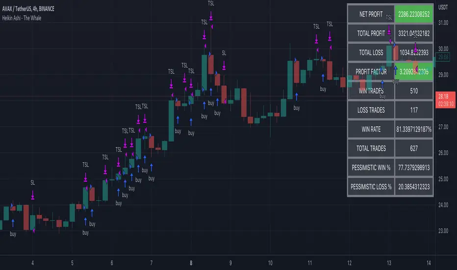
Heikin Ashi - The WhaleThe strategy is based on Heikin Ashi calculation, you do not need to switch the candle to HA.
The HA is used as a base entry, if a candle or two candles are bullish, then is valid to open a position, you can select the validation, one or two candles.
Also, the strategy mainly uses volume indicators as a confluence, you can select VWAP , VWMA , and Volume Oscillator, in addition to ADX which has two ways to validate the entry.
Base entry: One or two bullish HA candles (candles without a lower wick)
Confluence Indicators:
ADX: Will give a positive signal only if ADX is above the threshold, or if +DI is above -DI, or both.
VWAP: will give a positive signal if HA close is above VWAP.
VWMA: composite of 3 MA (20, 25, 50). There are multiple options to set it as confluence, the first option is to check if the short is bigger than the long and long is bigger than the base. The other options are to check the close status, which is bigger than which MA. You can find the description of each option in the strategy box
The sell is based on trailing stop loss (TSL), while the stop loss is based lowest X candle, the strategy will look back to the lowest number of the HA candles and set it as stop loss.
Heikin-ashi
MTF Heikinashi BarOVERVIEW
This indicator shows whether Heikin Ashi is up or down, represented by a bar. This indicator is compatible with MTF.
CONCEPTS
What do you want to know about market analysis?
Do you want a hard analysis? You can look for it.
All I want to know is whether the commonly known technical analysis is 'UP' or 'DOWN'.
All I want to know is whether the current market price is going up or down. Not only for the current, but also for the monthly, weekly, and daily status.
I want to make a decision in a moment. Without even thinking about it.
That is why I created a color-coded bar indicator to show the status.
No need to frown anymore.
DETAILS
Heikin means average. Ashi means legs. In this case, it means a candle.
Close = (Close + Open + High + Low) / 4
For more information, click here.
tradingview.com
Heikin Ashi Up ⇒ green
Heikin Ashi Down ⇒ red

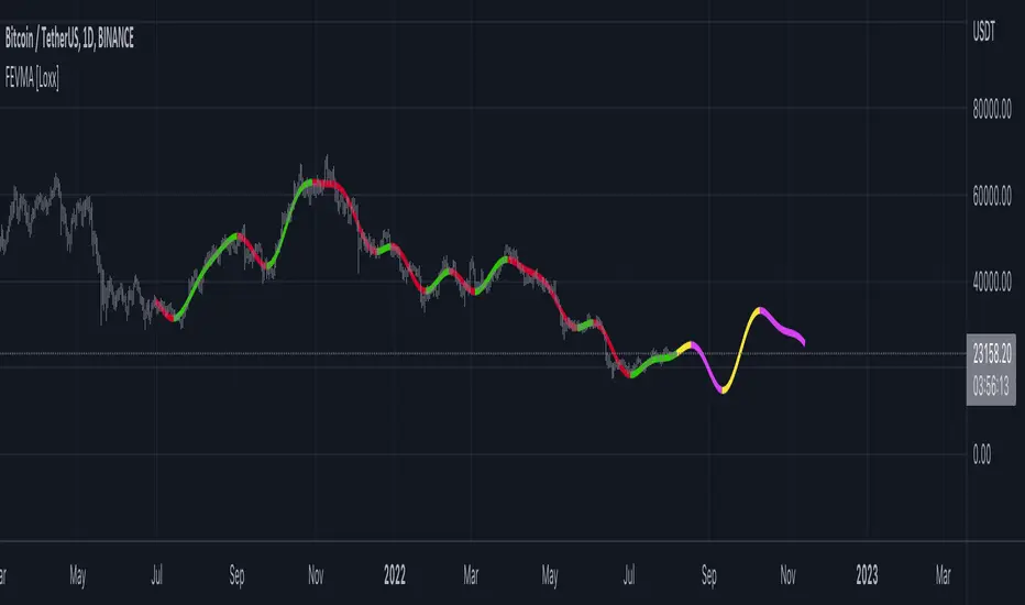
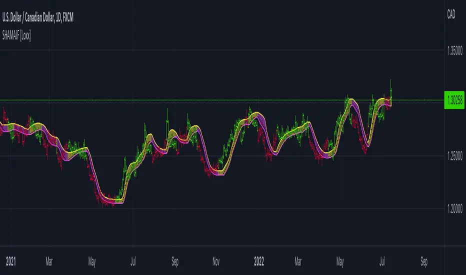
Fourier Extrapolation of Variety Moving Averages [Loxx]Fourier Extrapolation of Variety Moving Averages is a Fourier Extrapolation (forecasting) indicator that has for inputs 38 different types of moving averages along with 33 different types of sources for those moving averages. This is a forecasting indicator of the selected moving average of the selected price of the underlying ticker. This indicator will repaint, so past signals are only as valid as the current bar. This indicator allows for up to 1500 bars between past bars and future projection bars. If the indicator won't load on your chart. check the error message for details on how to fix that, but you must ensure that past bars + futures bars is equal to or less than 1500.
Fourier Extrapolation using the Quinn-Fernandes algorithm is one of several (5-10) methods of signals forecasting that I'l be demonstrating in Pine Script.
What is Fourier Extrapolation?
This indicator uses a multi-harmonic (or multi-tone) trigonometric model of a price series xi, i=1..n, is given by:
xi = m + Sum( a*Cos(w*i) + b*Sin(w*i), h=1..H )
Where:
xi - past price at i-th bar, total n past prices;
m - bias;
a and b - scaling coefficients of harmonics;
w - frequency of a harmonic ;
h - harmonic number;
H - total number of fitted harmonics.
Fitting this model means finding m, a, b, and w that make the modeled values to be close to real values. Finding the harmonic frequencies w is the most difficult part of fitting a trigonometric model. In the case of a Fourier series, these frequencies are set at 2*pi*h/n. But, the Fourier series extrapolation means simply repeating the n past prices into the future.
This indicator uses the Quinn-Fernandes algorithm to find the harmonic frequencies. It fits harmonics of the trigonometric series one by one until the specified total number of harmonics H is reached. After fitting a new harmonic , the coded algorithm computes the residue between the updated model and the real values and fits a new harmonic to the residue.
see here: A Fast Efficient Technique for the Estimation of Frequency , B. G. Quinn and J. M. Fernandes, Biometrika, Vol. 78, No. 3 (Sep., 1991), pp . 489-497 (9 pages) Published By: Oxford University Press
The indicator has the following input parameters:
src - input source
npast - number of past bars, to which trigonometric series is fitted;
Nfut - number of predicted future bars;
nharm - total number of harmonics in model;
frqtol - tolerance of frequency calculations.
Included:
Loxx's Expanded Source Types
Loxx's Moving Averages
Other indicators using this same method
Fourier Extrapolator of Variety RSI w/ Bollinger Bands
Fourier Extrapolator of Price w/ Projection Forecast
Fourier Extrapolator of Price
Loxx's Moving Averages: Detailed explanation of moving averages inside this indicator
Loxx's Expanded Source Types: Detailed explanation of source types used in this indicator
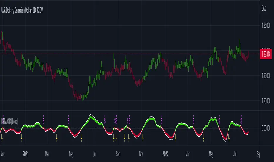
Hodrick-Prescott MACD [Loxx]Hodrick-Prescott MACD is a MACD indicator using a Hodrick-Prescott Filter.
What is Hodrick–Prescott filter?
The Hodrick–Prescott filter (also known as Hodrick–Prescott decomposition) is a mathematical tool used in macroeconomics, especially in real business cycle theory, to remove the cyclical component of a time series from raw data. It is used to obtain a smoothed-curve representation of a time series, one that is more sensitive to long-term than to short-term fluctuations. The adjustment of the sensitivity of the trend to short-term fluctuations is achieved by modifying a multiplier Lambda.
The filter was popularized in the field of economics in the 1990s by economists Robert J. Hodrick and Nobel Memorial Prize winner Edward C. Prescott, though it was first proposed much earlier by E. T. Whittaker in 1923.
There are some drawbacks to use the HP filter than you can read here: en.wikipedia.org
Included
Bar coloring
3 types of signals
Alerts
Loxx's Expanded Source Types
Stepped Moving Average of CCI [Loxx]Stepped Moving Average of CCI is a CCI that applies a stepping algorithm to smooth CCI. This allows for noice reduction and better identification of breakouts/breakdowns/reversals.
What is CCI?
The Commodity Channel Index ( CCI ) measures the current price level relative to an average price level over a given period of time. CCI is relatively high when prices are far above their average. CCI is relatively low when prices are far below their average. Using this method, CCI can be used to identify overbought and oversold levels.
Included:
Bar coloring
4 signal variations w/ alerts
Loxx's Expanded Source Types
Loxx's Moving Averages
T3 Velocity [Loxx]T3 Velocity is a simple velocity indicator using T3 moving average that uses gradient colors to better identify trends.
What is the T3 moving average?
Better Moving Averages Tim Tillson
November 1, 1998
Tim Tillson is a software project manager at Hewlett-Packard, with degrees in Mathematics and Computer Science. He has privately traded options and equities for 15 years.
Introduction
"Digital filtering includes the process of smoothing, predicting, differentiating, integrating, separation of signals, and removal of noise from a signal. Thus many people who do such things are actually using digital filters without realizing that they are; being unacquainted with the theory, they neither understand what they have done nor the possibilities of what they might have done."
This quote from R. W. Hamming applies to the vast majority of indicators in technical analysis . Moving averages, be they simple, weighted, or exponential, are lowpass filters; low frequency components in the signal pass through with little attenuation, while high frequencies are severely reduced.
"Oscillator" type indicators (such as MACD , Momentum, Relative Strength Index ) are another type of digital filter called a differentiator.
Tushar Chande has observed that many popular oscillators are highly correlated, which is sensible because they are trying to measure the rate of change of the underlying time series, i.e., are trying to be the first and second derivatives we all learned about in Calculus.
We use moving averages (lowpass filters) in technical analysis to remove the random noise from a time series, to discern the underlying trend or to determine prices at which we will take action. A perfect moving average would have two attributes:
It would be smooth, not sensitive to random noise in the underlying time series. Another way of saying this is that its derivative would not spuriously alternate between positive and negative values.
It would not lag behind the time series it is computed from. Lag, of course, produces late buy or sell signals that kill profits.
The only way one can compute a perfect moving average is to have knowledge of the future, and if we had that, we would buy one lottery ticket a week rather than trade!
Having said this, we can still improve on the conventional simple, weighted, or exponential moving averages. Here's how:
Two Interesting Moving Averages
We will examine two benchmark moving averages based on Linear Regression analysis.
In both cases, a Linear Regression line of length n is fitted to price data.
I call the first moving average ILRS, which stands for Integral of Linear Regression Slope. One simply integrates the slope of a linear regression line as it is successively fitted in a moving window of length n across the data, with the constant of integration being a simple moving average of the first n points. Put another way, the derivative of ILRS is the linear regression slope. Note that ILRS is not the same as a SMA ( simple moving average ) of length n, which is actually the midpoint of the linear regression line as it moves across the data.
We can measure the lag of moving averages with respect to a linear trend by computing how they behave when the input is a line with unit slope. Both SMA (n) and ILRS(n) have lag of n/2, but ILRS is much smoother than SMA .
Our second benchmark moving average is well known, called EPMA or End Point Moving Average. It is the endpoint of the linear regression line of length n as it is fitted across the data. EPMA hugs the data more closely than a simple or exponential moving average of the same length. The price we pay for this is that it is much noisier (less smooth) than ILRS, and it also has the annoying property that it overshoots the data when linear trends are present.
However, EPMA has a lag of 0 with respect to linear input! This makes sense because a linear regression line will fit linear input perfectly, and the endpoint of the LR line will be on the input line.
These two moving averages frame the tradeoffs that we are facing. On one extreme we have ILRS, which is very smooth and has considerable phase lag. EPMA has 0 phase lag, but is too noisy and overshoots. We would like to construct a better moving average which is as smooth as ILRS, but runs closer to where EPMA lies, without the overshoot.
A easy way to attempt this is to split the difference, i.e. use (ILRS(n)+EPMA(n))/2. This will give us a moving average (call it IE /2) which runs in between the two, has phase lag of n/4 but still inherits considerable noise from EPMA. IE /2 is inspirational, however. Can we build something that is comparable, but smoother? Figure 1 shows ILRS, EPMA, and IE /2.
Filter Techniques
Any thoughtful student of filter theory (or resolute experimenter) will have noticed that you can improve the smoothness of a filter by running it through itself multiple times, at the cost of increasing phase lag.
There is a complementary technique (called twicing by J.W. Tukey) which can be used to improve phase lag. If L stands for the operation of running data through a low pass filter, then twicing can be described by:
L' = L(time series) + L(time series - L(time series))
That is, we add a moving average of the difference between the input and the moving average to the moving average. This is algebraically equivalent to:
2L-L(L)
This is the Double Exponential Moving Average or DEMA , popularized by Patrick Mulloy in TASAC (January/February 1994).
In our taxonomy, DEMA has some phase lag (although it exponentially approaches 0) and is somewhat noisy, comparable to IE /2 indicator.
We will use these two techniques to construct our better moving average, after we explore the first one a little more closely.
Fixing Overshoot
An n-day EMA has smoothing constant alpha=2/(n+1) and a lag of (n-1)/2.
Thus EMA (3) has lag 1, and EMA (11) has lag 5. Figure 2 shows that, if I am willing to incur 5 days of lag, I get a smoother moving average if I run EMA (3) through itself 5 times than if I just take EMA (11) once.
This suggests that if EPMA and DEMA have 0 or low lag, why not run fast versions (eg DEMA (3)) through themselves many times to achieve a smooth result? The problem is that multiple runs though these filters increase their tendency to overshoot the data, giving an unusable result. This is because the amplitude response of DEMA and EPMA is greater than 1 at certain frequencies, giving a gain of much greater than 1 at these frequencies when run though themselves multiple times. Figure 3 shows DEMA (7) and EPMA(7) run through themselves 3 times. DEMA^3 has serious overshoot, and EPMA^3 is terrible.
The solution to the overshoot problem is to recall what we are doing with twicing:
DEMA (n) = EMA (n) + EMA (time series - EMA (n))
The second term is adding, in effect, a smooth version of the derivative to the EMA to achieve DEMA . The derivative term determines how hot the moving average's response to linear trends will be. We need to simply turn down the volume to achieve our basic building block:
EMA (n) + EMA (time series - EMA (n))*.7;
This is algebraically the same as:
EMA (n)*1.7-EMA( EMA (n))*.7;
I have chosen .7 as my volume factor, but the general formula (which I call "Generalized Dema") is:
GD (n,v) = EMA (n)*(1+v)-EMA( EMA (n))*v,
Where v ranges between 0 and 1. When v=0, GD is just an EMA , and when v=1, GD is DEMA . In between, GD is a cooler DEMA . By using a value for v less than 1 (I like .7), we cure the multiple DEMA overshoot problem, at the cost of accepting some additional phase delay. Now we can run GD through itself multiple times to define a new, smoother moving average T3 that does not overshoot the data:
T3(n) = GD ( GD ( GD (n)))
In filter theory parlance, T3 is a six-pole non-linear Kalman filter. Kalman filters are ones which use the error (in this case (time series - EMA (n)) to correct themselves. In Technical Analysis , these are called Adaptive Moving Averages; they track the time series more aggressively when it is making large moves.
Included:
Bar coloring
Signals
Alerts
Loxx's Expanded Source Types

PPO w/ Discontinued Signal Lines [Loxx]PPO w/ Discontinued Signal Lines is a Percentage Price Oscillator with some upgrades. This indicator has 33 source types and 35+ moving average types as well as Discontinued Signal Lines and divergences. These additions reduce noise and increase hit rate.
What is the Price Percentage Oscillator?
The percentage price oscillator (PPO) is a technical momentum indicator that shows the relationship between two moving averages in percentage terms. The moving averages are a 26-period and 12-period exponential moving average (EMA).
The PPO is used to compare asset performance and volatility, spot divergence that could lead to price reversals, generate trade signals, and help confirm trend direction.
Included:
Bar coloring
3 signal variations w/ alerts
Divergences w/ alerts
Loxx's Expanded Source Types
Loxx's Moving Averages

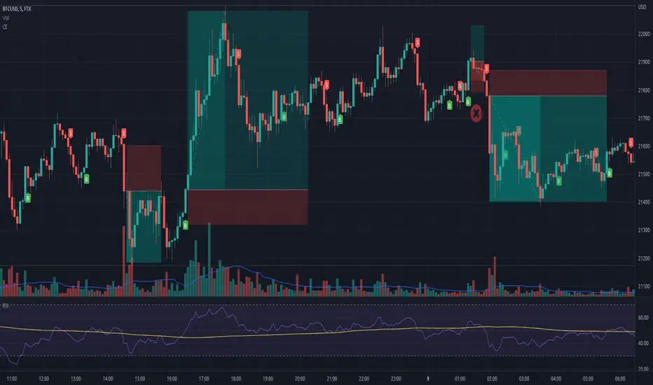
Smoothed Heikin Ashi Trend on Chart - TraderHalai BACKTESTSmoothed Heikin Ashi Trend on chart - Backtest
This is a backtest of the Smoothed Heikin Ashi Trend indicator, which computes the reverse candle close price required to flip a Heikin Ashi trend from red to green and vice versa. The original indicator can be found in the scripts section of my profile.
This particular back test uses this indicator with a Trend following paradigm with a percentage-based stop loss.
Note, that backtesting performance is not always indicative of future performance, but it does provide some basis for further development and walk-forward / live testing.
Testing was performed on Bitcoin , as this is a primary target market for me to use this kind of strategy.
Sample Backtesting results as of 10th June 2022:
Backtesting parameters:
Position size: 10% of equity
Long stop: 1% below entry
Short stop: 1% above entry
Repainting: Off
Smoothing: SMA
Period: 10
8 Hour:
Number of Trades: 1046
Gross Return: 249.27 %
CAGR Return: 14.04 %
Max Drawdown: 7.9 %
Win percentage: 28.01 %
Profit Factor (Expectancy): 2.019
Average Loss: 0.33 %
Average Win: 1.69 %
Average Time for Loss: 1 day
Average Time for Win: 5.33 days
1 Day:
Number of Trades: 429
Gross Return: 458.4 %
CAGR Return: 15.76 %
Max Drawdown: 6.37 %
Profit Factor (Expectancy): 2.804
Average Loss: 0.8 %
Average Win: 7.2 %
Average Time for Loss: 3 days
Average Time for Win: 16 days
5 Day:
Number of Trades: 69
Gross Return: 1614.9 %
CAGR Return: 26.7 %
Max Drawdown: 5.7 %
Profit Factor (Expectancy): 10.451
Average Loss: 3.64 %
Average Win: 81.17 %
Average Time for Loss: 15 days
Average Time for Win: 85 days
Analysis:
The strategy is typical amongst trend following strategies with a less regular win rate, but where profits are more significant than losses. Most of the losses are in sideways, low volatility markets. This strategy performs better on higher timeframes, where it shows a positive expectancy of the strategy.
The average win was positively impacted by Bitcoin’s earlier smaller market cap, as the percentage wins earlier were higher.
Overall the strategy shows potential for further development and may be suitable for walk-forward testing and out of sample analysis to be considered for a demo trading account.
Note in an actual trading setup, you may wish to use this with volatility filters, combined with support resistance zones for a better setup.
As always, this post/indicator/strategy is not financial advice, and please do your due diligence before trading this live.
Original indicator links:
On chart version -
Oscillator version -
Update - 27/06/2022
Unfortunately, It appears that the original script had been taken down due to auto-moderation because of concerns with no slippage / commission. I have since adjusted the backtest, and re-uploaded to include the following to address these concerns, and show that I am genuinely trying to give back to the community and not mislead anyone:
1) Include commission of 0.1% - to match Binance's maker fees prior to moving to a fee-less model.
2) Include slippage of 10 ticks (This is a realistic slippage figure from searching online for most crypto exchanges)
3) Adjust account balance to 10,000 - since most of us are not millionaires.
The rest of the backtesting parameters are comparable to previous results:
Backtesting parameters:
Initial capital: 10000 dollars
Position size: 10% of equity
Long stop: 2% below entry
Short stop: 2% above entry
Repainting: Off
Smoothing: SMA
Period: 10
Slippage: 10 ticks
Commission: 0.1%
This script still remains to shows viability / profitablity on higher term timeframes (with slightly higher drawdown), and I have included the backtest report below to document my findings:
8 Hour:
Number of Trades: 1082
Gross Return: 233.02%
CAGR Return: 14.04 %
Max Drawdown: 7.9 %
Win percentage: 25.6%
Profit Factor (Expectancy): 1.627
Average Loss: 0.46 %
Average Win: 2.18 %
Average Time for Loss: 1.33 day
Average Time for Win: 7.33 days
Once again, please do your own research and due dillegence before trading this live. This post is for education and information purposes only, and should not be taken as financial advice.

R-sqrd Adapt. Fisher Transform w/ D. Zones & Divs. [Loxx]The full name of this indicator is R-Squared Adaptive Fisher Transform w/ Dynamic Zones and Divergences. This is an R-squared adaptive Fisher transform with adjustable dynamic zones, signals, alerts, and divergences.
What is Fisher Transform?
The Fisher Transform is a technical indicator created by John F. Ehlers that converts prices into a Gaussian normal distribution.
The indicator highlights when prices have moved to an extreme, based on recent prices. This may help in spotting turning points in the price of an asset. It also helps show the trend and isolate the price waves within a trend.
What is R-squared Adaptive?
One tool available in forecasting the trendiness of the breakout is the coefficient of determination ( R-squared ), a statistical measurement.
The R-squared indicates linear strength between the security's price (the Y - axis) and time (the X - axis). The R-squared is the percentage of squared error that the linear regression can eliminate if it were used as the predictor instead of the mean value. If the R-squared were 0.99, then the linear regression would eliminate 99% of the error for prediction versus predicting closing prices using a simple moving average .
R-squared is used here to derive an r-squared value that is then modified by a user input "factor"
What are Dynamic Zones?
As explained in "Stocks & Commodities V15:7 (306-310): Dynamic Zones by Leo Zamansky, Ph .D., and David Stendahl"
Most indicators use a fixed zone for buy and sell signals. Here’ s a concept based on zones that are responsive to past levels of the indicator.
One approach to active investing employs the use of oscillators to exploit tradable market trends. This investing style follows a very simple form of logic: Enter the market only when an oscillator has moved far above or below traditional trading lev- els. However, these oscillator- driven systems lack the ability to evolve with the market because they use fixed buy and sell zones. Traders typically use one set of buy and sell zones for a bull market and substantially different zones for a bear market. And therein lies the problem.
Once traders begin introducing their market opinions into trading equations, by changing the zones, they negate the system’s mechanical nature. The objective is to have a system automatically define its own buy and sell zones and thereby profitably trade in any market — bull or bear. Dynamic zones offer a solution to the problem of fixed buy and sell zones for any oscillator-driven system.
An indicator’s extreme levels can be quantified using statistical methods. These extreme levels are calculated for a certain period and serve as the buy and sell zones for a trading system. The repetition of this statistical process for every value of the indicator creates values that become the dynamic zones. The zones are calculated in such a way that the probability of the indicator value rising above, or falling below, the dynamic zones is equal to a given probability input set by the trader.
To better understand dynamic zones, let's first describe them mathematically and then explain their use. The dynamic zones definition:
Find V such that:
For dynamic zone buy: P{X <= V}=P1
For dynamic zone sell: P{X >= V}=P2
where P1 and P2 are the probabilities set by the trader, X is the value of the indicator for the selected period and V represents the value of the dynamic zone.
The probability input P1 and P2 can be adjusted by the trader to encompass as much or as little data as the trader would like. The smaller the probability, the fewer data values above and below the dynamic zones. This translates into a wider range between the buy and sell zones. If a 10% probability is used for P1 and P2, only those data values that make up the top 10% and bottom 10% for an indicator are used in the construction of the zones. Of the values, 80% will fall between the two extreme levels. Because dynamic zone levels are penetrated so infrequently, when this happens, traders know that the market has truly moved into overbought or oversold territory.
Calculating the Dynamic Zones
The algorithm for the dynamic zones is a series of steps. First, decide the value of the lookback period t. Next, decide the value of the probability Pbuy for buy zone and value of the probability Psell for the sell zone.
For i=1, to the last lookback period, build the distribution f(x) of the price during the lookback period i. Then find the value Vi1 such that the probability of the price less than or equal to Vi1 during the lookback period i is equal to Pbuy. Find the value Vi2 such that the probability of the price greater or equal to Vi2 during the lookback period i is equal to Psell. The sequence of Vi1 for all periods gives the buy zone. The sequence of Vi2 for all periods gives the sell zone.
In the algorithm description, we have: Build the distribution f(x) of the price during the lookback period i. The distribution here is empirical namely, how many times a given value of x appeared during the lookback period. The problem is to find such x that the probability of a price being greater or equal to x will be equal to a probability selected by the user. Probability is the area under the distribution curve. The task is to find such value of x that the area under the distribution curve to the right of x will be equal to the probability selected by the user. That x is the dynamic zone.
Included:
Bar coloring
4 signal variations w/ alerts
Divergences w/ alerts
Loxx's Expanded Source Types
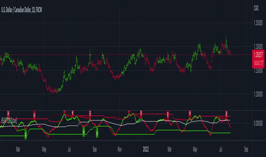
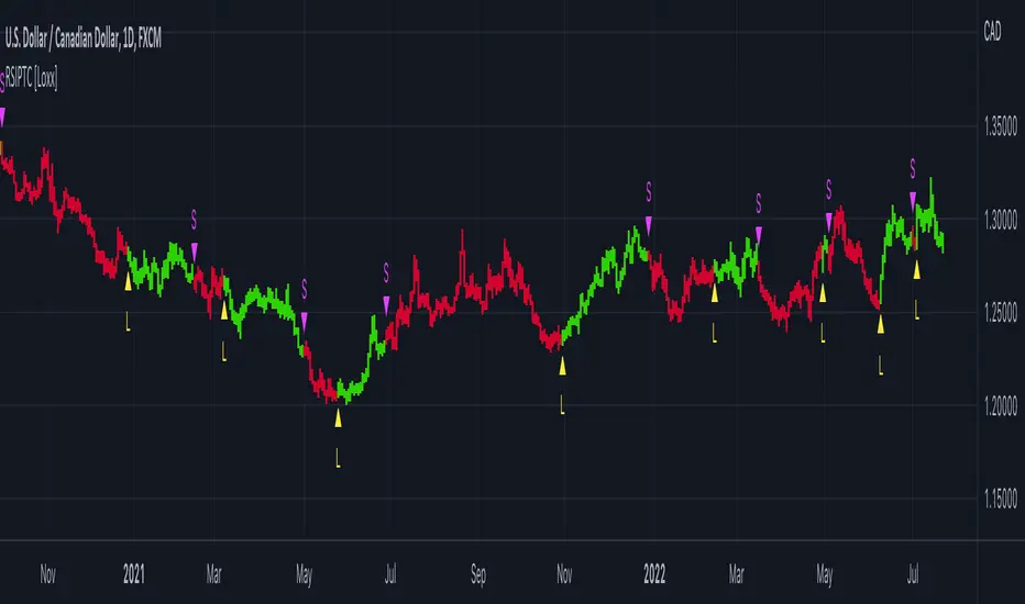
RSI Precision Trend Candles [Loxx]RSI Precision Trend Candles is a candle coloring indicator that uses an average range algorithm to determine trend direction. The precision trend algorithm can be used on any calculated output to tease out interesting trend information.
What is RSI?
The relative strength index (RSI) is a momentum indicator used in technical analysis. RSI measures the speed and magnitude of a security's recent price changes to evaluate overvalued or undervalued conditions in the price of that security.
The RSI is displayed as an oscillator (a line graph) on a scale of zero to 100. The indicator was developed by J. Welles Wilder Jr. and introduced in his seminal 1978 book, New Concepts in Technical Trading Systems.
Included
Bar coloring
Signals
Alerts
Loxx's Expanded Source Types
Variety Moving Averages w/ Dynamic Zones [Loxx]Variety Moving Averages w/ Dynamic Zones contains 33 source types and 35+ moving averages with double dynamic zones levels.
What are Dynamic Zones?
As explained in "Stocks & Commodities V15:7 (306-310): Dynamic Zones by Leo Zamansky, Ph .D., and David Stendahl"
Most indicators use a fixed zone for buy and sell signals. Here’ s a concept based on zones that are responsive to past levels of the indicator.
One approach to active investing employs the use of oscillators to exploit tradable market trends. This investing style follows a very simple form of logic: Enter the market only when an oscillator has moved far above or below traditional trading lev- els. However, these oscillator- driven systems lack the ability to evolve with the market because they use fixed buy and sell zones. Traders typically use one set of buy and sell zones for a bull market and substantially different zones for a bear market. And therein lies the problem.
Once traders begin introducing their market opinions into trading equations, by changing the zones, they negate the system’s mechanical nature. The objective is to have a system automatically define its own buy and sell zones and thereby profitably trade in any market — bull or bear. Dynamic zones offer a solution to the problem of fixed buy and sell zones for any oscillator-driven system.
An indicator’s extreme levels can be quantified using statistical methods. These extreme levels are calculated for a certain period and serve as the buy and sell zones for a trading system. The repetition of this statistical process for every value of the indicator creates values that become the dynamic zones. The zones are calculated in such a way that the probability of the indicator value rising above, or falling below, the dynamic zones is equal to a given probability input set by the trader.
To better understand dynamic zones, let's first describe them mathematically and then explain their use. The dynamic zones definition:
Find V such that:
For dynamic zone buy: P{X <= V}=P1
For dynamic zone sell: P{X >= V}=P2
where P1 and P2 are the probabilities set by the trader, X is the value of the indicator for the selected period and V represents the value of the dynamic zone.
The probability input P1 and P2 can be adjusted by the trader to encompass as much or as little data as the trader would like. The smaller the probability, the fewer data values above and below the dynamic zones. This translates into a wider range between the buy and sell zones. If a 10% probability is used for P1 and P2, only those data values that make up the top 10% and bottom 10% for an indicator are used in the construction of the zones. Of the values, 80% will fall between the two extreme levels. Because dynamic zone levels are penetrated so infrequently, when this happens, traders know that the market has truly moved into overbought or oversold territory.
Calculating the Dynamic Zones
The algorithm for the dynamic zones is a series of steps. First, decide the value of the lookback period t. Next, decide the value of the probability Pbuy for buy zone and value of the probability Psell for the sell zone.
For i=1, to the last lookback period, build the distribution f(x) of the price during the lookback period i. Then find the value Vi1 such that the probability of the price less than or equal to Vi1 during the lookback period i is equal to Pbuy. Find the value Vi2 such that the probability of the price greater or equal to Vi2 during the lookback period i is equal to Psell. The sequence of Vi1 for all periods gives the buy zone. The sequence of Vi2 for all periods gives the sell zone.
In the algorithm description, we have: Build the distribution f(x) of the price during the lookback period i. The distribution here is empirical namely, how many times a given value of x appeared during the lookback period. The problem is to find such x that the probability of a price being greater or equal to x will be equal to a probability selected by the user. Probability is the area under the distribution curve. The task is to find such value of x that the area under the distribution curve to the right of x will be equal to the probability selected by the user. That x is the dynamic zone.
Included
Bar coloring
Alerts
Channels fill
Loxx's Expanded Source Types
35+ moving average types

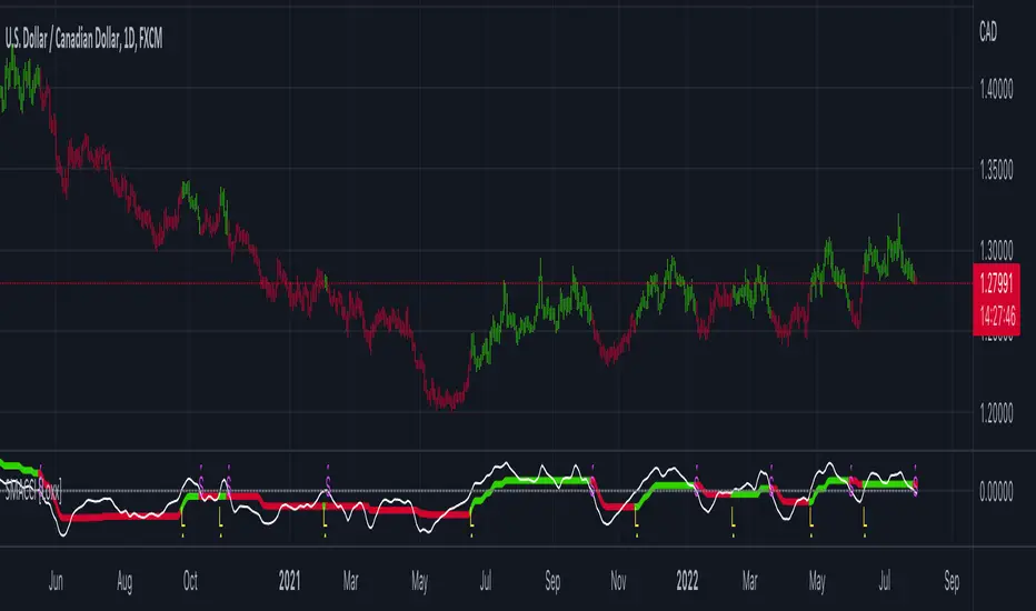
Smoothed RSI Heikin Ashi Oscillator w/ Expanded Types [Loxx]Smoothed RSI Heikin-Ashi Oscillator w/ Expanded Types is a spin on Heikin Ashi RSI Oscillator by @JayRogers. The purpose of this modification is to reduce noise in the original version thereby increasing suitability of the signal output. This indicator is tuned for Forex markets.
Differences:
35+ Smoothing Options for RSI
35+ Smoothing Options for HA Candles
Heiken-Ashi Better Expanded Source input. This source input is use for the RSI calculation only.
Signals
Alerts
What are Heiken-Ashi "better" candles?
The "better formula" was proposed in an article/memo by BNP-Paribas (In Warrants & Zertifikate, No. 8, August 2004 (a monthly German magazine published by BNP Paribas, Frankfurt), there is an article by Sebastian Schmidt about further development (smoothing) of Heikin-Ashi chart.)
They proposed to use the following :
(Open+Close)/2+(((Close-Open)/( High-Low ))*ABS((Close-Open)/2))
instead of using :
haClose = (O+H+L+C)/4
According to that document the HA representation using their proposed formula is better than the traditional formula.
What are traditional Heiken-Ashi candles?
The Heikin-Ashi technique averages price data to create a Japanese candlestick chart that filters out market noise.
Heikin-Ashi charts, developed by Munehisa Homma in the 1700s, share some characteristics with standard candlestick charts but differ based on the values used to create each candle. Instead of using the open, high, low, and close like standard candlestick charts, the Heikin-Ashi technique uses a modified formula based on two-period averages. This gives the chart a smoother appearance, making it easier to spots trends and reversals, but also obscures gaps and some price data.
Future updates
Expand signal options to include RSI-, Zero-, and color-crosses

VHF-Adaptive T3 w/ Expanded Source Types [Loxx]VHF-Adaptive T3 w/ Expanded Source Types is a T3 moving average with expanded source types and adaptive period inputs using a vertical horizontal filter
What is T3?
Developed by Tim Tillson, the T3 Moving Average is considered superior to traditional moving averages as it is smoother, more responsive and thus performs better in ranging market conditions as well.
What is VHF Adaptive Cycle?
Vertical Horizontal Filter (VHF) was created by Adam White to identify trending and ranging markets. VHF measures the level of trend activity, similar to ADX DI. Vertical Horizontal Filter does not, itself, generate trading signals, but determines whether signals are taken from trend or momentum indicators. Using this trend information, one is then able to derive an average cycle length.
Included
Bar coloring
Alerts
Loxx's Expanded Source Types

Candle Stick UpdateHeikin ashi chart so powerful that you can understand trend direction easily. But sometimes, this type of chart doesn't update properly and make no sense on real time. So I made this script. You can now change candle stick style default to heikin ashi (default / modified version) on the real time default chart without switching heikin ashi chart. Enjoy traders!!! And don't forget to press the like button :)

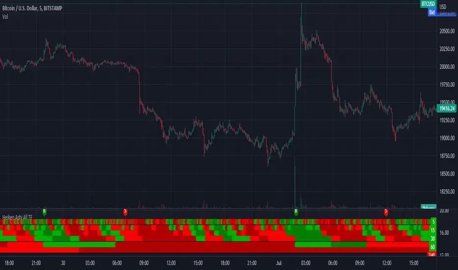
Heiken Ashi All TFI have always fighted to understand the market direction because it looks different on different timeframes.
I wanted an indicator where I can see all the different timeframes at once.
This indicator shows the Heiken Ashi candle colors for different time frames at once.
Use it on the 5 Minute timeframe.
4 colors:
dark green: bullis green HA candle with no low shadow.
green: green HA candle.
red: red HA candle
datk red: bearish red HA candle with non existing upper shadow.
the timeframes are by default:
5m 15m 30m 1H 4H 1D
can be adjusted if needed.
signals:
in the top line the Buy / Shell Signals are shown when the selected timeframes are all changed.
for example after a buy signal a sell signal will be printend when all the selected timeframes are turned into red or dark red.
Do not use it as a tranding signal, us it for confirmation.
It doesn't predict. it shows the market's current state.
Don't forget that the latest candles are based on the current value. The higher timeframe candle color depends on the current price.
If the higher timeframe close price so different that the HA candle color changes it reprins for all the affected 5m dots.
Stepped Heiken Ashi Moving Average w/ Jurik Filtering [Loxx]Stepped Heiken Ashi Moving Average w/ Jurik Filtering is a Heiken Ashi moving average with Jurik Filtering and stepping by pips. This can be used as a moving average channel.
What is Jurik Volty used in the Juirk Filter?
One of the lesser known qualities of Juirk smoothing is that the Jurik smoothing process is adaptive. "Jurik Volty" (a sort of market volatility ) is what makes Jurik smoothing adaptive. The Jurik Volty calculation can be used as both a standalone indicator and to smooth other indicators that you wish to make adaptive.
What is the Jurik Moving Average?
Have you noticed how moving averages add some lag (delay) to your signals? ... especially when price gaps up or down in a big move, and you are waiting for your moving average to catch up? Wait no more! JMA eliminates this problem forever and gives you the best of both worlds: low lag and smooth lines.
Included:
Toggle fill color
Toggle bar color
Toggle candles
Heikin Ashi Volatility Percentile - TraderHalaiThe Heikin Ashi Volatility Percentile (HAVP) Oscillator was inspired by the legendary Bollinger Band Width Percentile indicator(known as BBWP), written by Caretaker, and made famous by Eric Krown, a famous influencer.
This script borrows aspects of the BBWP indicator which enables the HAVP oscillator to visually match the look and feel of BBWP and allows similar configuration functions (such as colouring function, smoothing MAs and alerts)
The fundamentals of this script are however different to BBWP. Instead of Bollinger band width, this script uses a reverse function of Heikin Ashi close (implemented in my Smoothed Heikin Ashi Trend
indicator, linked below).
The reverse Heikin Ashi close is smoothed using Ehler's SuperSmoother function, providing smooth oscillation and earlier signals of volatility tops and bottoms.
From an automated backtest that I have conducted on the BTCUSD index pair, I have observed comparable performance to BBWP across multiple timeframes when combining with stochastic direction to give a bias on overall direction. Using parameters I have tested, it performs better on mid-term timeframes such as 3h,4h and 6h. BBWP outperforms on 1h and 1d, with lower timeframes being comparable.
From the results, using HAVP over BBWP tends to result in reduced holding time and more frequent trades, which may or may not be desirable, although the behaviour can be adjusted using the parameters provided.
For instance, the smoother oscillation provided by HAVP provides a great predictability factor and earlier confirmation signals, which is something that Ehler emphasised in his trading style, and something which I agree with personally. I would encourage you to try out both HAVP and BBWP and see which fits your trading style.
Releasing this as open source allows for the betterment of the community and further development, criticism and discussion.
Thanks and enjoy! :)

Chandelier Exit - Heikin AshiThis is a redesign of the Chandelier Exit indicator. It removes stupid transitions between Chandelier Exit' states and highlights initial points for both lines.
This indicator was originally developed by Charles Le Beau and popularized by Dr . Alexander Elder in his book "Come Into My Trading Room: A Complete Guide to Trading" (2002).
In short, this is a trailing stop-loss based on the Average True Range (ATR).
If "Heikin Ashi for calculation" is checked, then ATR and buy/sell signals are calculated based on heikin ashi candles.
You don't need to change bar style to heikin ashi.
Thanks to everget for the initial version.
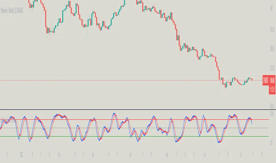
ARKA-Heikin Ashi OscillatorThis Indicator is based on Mr. Dan Valcu ideas.
This indicator is made as Hicken-Ashi Oscillator by haDelta. The closing price of the candlestick is not used to make this indicator.
- Indicators generally have a delay. Since this indicator has an haDelta oscillator, it helps to reduce this delay.
- This indicator has two fast lines "K" and slow "D".
-Similarly to haDelta, this indicator can be used to calculate price targets based on inverse positive and negative divergences between the price and the oscillator.
- The peaks or lows range in the oscillator is almost the oversold and overbought points in the price chart.
- Use this oscillator similar to other oscillators and use the oversold and overbought levels, 50-level, divergences and crossovers between its two components.
-In an uptrend, when the oscillator turns down, it is time to reduce the stop loss on long trades.
-In a downtrend, when the oscillator is bullish , it is time to reduce the stop loss on short trades.
loxxexpandedsourcetypesLibrary "loxxexpandedsourcetypes"
Expanded source types used in Loxx's indicators and strategies.
rclose()
rClose: regular close
Returns: float
ropen()
rClose: regular open
Returns: float
rhigh()
rClose: regular high
Returns: float
rlow()
rClose: regular low
Returns: float
rmedian()
rClose: regular hl2
Returns: float
rtypical()
rClose: regular hlc3
Returns: float
rweighted()
rClose: regular hlcc4
Returns: float
raverage()
rClose: regular ohlc4
Returns: float
ravemedbody()
rClose: median body
Returns: float
rtrendb()
rClose: trend regular
Returns: float
rtrendbext()
rClose: trend extreme
Returns: float
haclose(haclose)
haclose: heiken-ashi close
Parameters:
haclose : float
Returns: float
haopen(haopen)
haopen: heiken-ashi open
Parameters:
haopen : float
Returns: float
hahigh(hahigh)
hahigh: heiken-ashi high
Parameters:
hahigh : float
Returns: float
halow(halow)
halow: heiken-ashi low
Parameters:
halow : float
Returns: float
hamedian(hamedian)
hamedian: heiken-ashi median
Parameters:
hamedian : float
Returns: float
hatypical(hatypical)
hatypical: heiken-ashi typical
Parameters:
hatypical : float
Returns: float
haweighted(haweighted)
haweighted: heiken-ashi weighted
Parameters:
haweighted : float
Returns: float
haaverage(haweighted)
haaverage: heiken-ashi average
Parameters:
haweighted : float
Returns: float
haavemedbody(haclose, haopen)
haavemedbody: heiken-ashi median body
Parameters:
haclose : float
haopen : float
Returns: float
hatrendb(haclose, haopen, hahigh, halow)
hatrendb: heiken-ashi trend
Parameters:
haclose : float
haopen : float
hahigh : float
halow : float
Returns: float
hatrendbext(haclose, haopen, hahigh, halow)
hatrendext: heiken-ashi trend extreme
Parameters:
haclose : float
haopen : float
hahigh : float
halow : float
Returns: float
habclose(smthtype, amafl, amasl, kfl, ksl)
habclose: heiken-ashi better open
Parameters:
smthtype : string
amafl : int
amasl : int
kfl : int
ksl : int
Returns: float
habopen(smthtype, amafl, amasl, kfl, ksl)
habopen: heiken-ashi better open
Parameters:
smthtype : string
amafl : int
amasl : int
kfl : int
ksl : int
Returns: float
habhigh(smthtype, amafl, amasl, kfl, ksl)
habhigh: heiken-ashi better high
Parameters:
smthtype : string
amafl : int
amasl : int
kfl : int
ksl : int
Returns: float
hablow(smthtype, amafl, amasl, kfl, ksl)
hablow: heiken-ashi better low
Parameters:
smthtype : string
amafl : int
amasl : int
kfl : int
ksl : int
Returns: float
habmedian(smthtype, amafl, amasl, kfl, ksl)
habmedian: heiken-ashi better median
Parameters:
smthtype : string
amafl : int
amasl : int
kfl : int
ksl : int
Returns: float
habtypical(smthtype, amafl, amasl, kfl, ksl)
habtypical: heiken-ashi better typical
Parameters:
smthtype : string
amafl : int
amasl : int
kfl : int
ksl : int
Returns: float
habweighted(smthtype, amafl, amasl, kfl, ksl)
habweighted: heiken-ashi better weighted
Parameters:
smthtype : string
amafl : int
amasl : int
kfl : int
ksl : int
Returns: float
habaverage(smthtype, amafl, amasl, kfl, ksl)
habaverage: heiken-ashi better average
Parameters:
smthtype : string
amafl : int
amasl : int
kfl : int
ksl : int
Returns: float
habavemedbody(smthtype, amafl, amasl, kfl, ksl)
habavemedbody: heiken-ashi better median body
Parameters:
smthtype : string
amafl : int
amasl : int
kfl : int
ksl : int
Returns: float
habtrendb(smthtype, amafl, amasl, kfl, ksl)
habtrendb: heiken-ashi better trend
Parameters:
smthtype : string
amafl : int
amasl : int
kfl : int
ksl : int
Returns: float
habtrendbext(smthtype, amafl, amasl, kfl, ksl)
habtrendbext: heiken-ashi better trend extreme
Parameters:
smthtype : string
amafl : int
amasl : int
kfl : int
ksl : int
Returns: float

Aarika Heikin AshiHello Traders,
This indicator is probably based for the people who use HA candlestick chart and frequently have to switch between Japanese candlestick and HA candles. The worry is over with this simple indicator.
Now you can enjoy both candlesticks at the same time.
AHA allows you to have 2 EMAs (mostly used for crossovers). Default values set at 8/21 EMA which we may indicate a trend reversal.
We strongly recommend you back-test everything that you need before you start using AHA.
Thank you.

Heikin Ashi CandlesLibrary "heikin_ashi_candles"
This library is programmed to calculate the Heikin Ashi candles using the standard formula of Heikin Ashi Candles.
Notice the Heikin Ashi chart type isn't 100% like the results from this calculation.
You can import this library in your code to use it as a smoothing method for your strategy which operates on the standard chart type.
_close()
_open()
_high()
_low()
_ohlc4()
_hlcc4()
_hlc3()
_hl2()

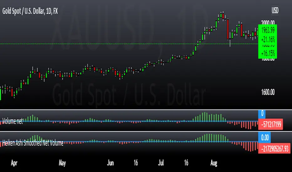
Heiken Ashi Smoothed Net VolumeThis indicator attempts to use Heiken Ashi calculations to smooth the Volume net histogram indicator by RafaelZioni. Long above zero line, short below zero line.