50-Line Oscillator // (\_/)
// ( •.•)
// (")_(")
25-Line Oscillator
Description:
The 25-Line Oscillator is a sophisticated technical analysis tool designed to visualize market trends through the use of multiple Simple Moving Averages (SMAs). This indicator computes a series of 26 SMAs, incrementally increasing the base length, providing traders with a comprehensive view of price dynamics.
Features:
Customizable Base Length: Adjust the base length of the SMAs according to trading preferences, enhancing versatility for different market conditions.
Rainbow Effect: The indicator employs a visually appealing rainbow color scheme to differentiate between the various trend lines, making it easy to identify crossovers and momentum shifts.
Crossovers Detection: The script includes logic to detect crossover events between consecutive trend lines, which can serve as signals for potential entry or exit points in trading.
Clear Visualization: Suitable for both novice and seasoned traders, the plots enable quick interpretation of trends and market behavior.
How to Use:
Add the indicator to your chart and customize the base length as desired.
Observe the rainbow-colored lines for trend direction.
Look for crossover events between the SMAs as potential trading signals.
Application: This indicator is particularly useful for swing traders and trend followers who aim to capitalize on market momentum and identify reversals. By monitoring the behavior of multiple SMAs, traders can gain insights into the strength and direction of price movements over various time frames.
Search in scripts for "oscillator"

DAMA OSC - Directional Adaptive MA OscillatorOverview:
The DAMA OSC (Directional Adaptive MA Oscillator) is a highly customizable and versatile oscillator that analyzes the delta between two moving averages of your choice. It detects trend progression, regressions, rebound signals, MA cross and critical zone crossovers to provide highly contextual trading information.
Designed for trend-following, reversal timing, and volatility filtering, DAMA OSC adapts to market conditions and highlights actionable signals in real-time.
Features:
Support for 11 custom moving average types (EMA, DEMA, TEMA, ALMA, KAMA, etc.)
Customizable fast & slow MA periods and types
Histogram based on percentage delta between fast and slow MA
Trend direction coloring with “Green”, “Blue”, and “Red” zones
Rebound detection using close or shadow logic
Configurable thresholds: Overbought, Oversold, Underbought, Undersold
Optional filters: rebound validation by candle color or flat-zone filter
Full visual overlay: MA lines, crossover markers, rebound icons
Complete alert system with 16 preconfigured conditions
How It Works:
Histogram Logic:
The histogram measures the percentage difference between the fast and slow MA:
hist_value = ((FastMA - SlowMA) / SlowMA) * 100
Trend State Logic (Green / Blue / Red):
Green_Up = Bullish acceleration
Blue_Up (or Red_Up, depending the display settings) = Bullish deceleration
Blue_Down (or Green_Down, depending the display settings) = Bearish deceleration
Red_Down = Bearish acceleration
Rebound Logic:
A rebound is detected when price:
Crosses back over a selected MA (fast or slow)
After being away for X candles (rebound_backstep)
Optional: filtered by histogram zones or candle color
Inputs:
Display Options:
Show/hide MA lines
Show/hide MA crosses
Show/hide price rebounds
Enable/disable blue deceleration zones
DAMA Settings:
Fast/Slow MA type and length
Source input (close by default)
Overbought/Oversold levels
Underbought/Undersold levels
Rebound Settings:
Use Close and/or Shadow
Rebound MA (Fast/Slow)
Candle color validation
Flat zone filter rebounds (between UnderSold and UnderBought)
Available MA type:
SMA (Simple MA)
EMA (Exponential MA)
DEMA (Double EMA)
TEMA (Triple EMA)
WMA (Weighted MA)
HMA (Hull MA)
VWMA (Volume Weighted MA)
Kijun (Ichimoku Baseline)
ALMA (Arnaud Legoux MA)
KAMA (Kaufman Adaptive MA)
HULLMOD (Modified Hull MA, Same as HMA, tweaked for Pine v6 constraints)
Notes:
**DEMA/TEMA** reduce lag compared to EMA, useful for faster reaction in trending markets.
**KAMA/ALMA** are better suited to noisy or volatile environments (e.g., BTC).
**VWMA** reacts strongly to volume spikes.
**HMA/HULLMOD** are great for visual clarity in fast moves.
Alerts Included (Fully Configurable):
Golden Cross:
Fast MA crosses above Slow MA
Death Cross:
Fast MA crosses below Slow MA
Bullish Rebound:
Rebound from below MA in uptrend
Bearish Rebound:
Rebound from above MA in downtrend
Bull Progression:
Transition into Green_Up with positive delta
Bear Progression:
Transition into Red_Down with negative delta
Bull Regression:
Exit from Red_Down into Blue/Green with negative delta
Bear Regression:
Exit from Green_Up into Blue/Red with positive delta
Crossover Overbought:
Histogram crosses above Overbought
Crossunder Overbought:
Histogram crosses below Overbought
Crossover Oversold:
Histogram crosses above Oversold
Crossunder Oversold:
Histogram crosses below Oversold
Crossover Underbought:
Histogram crosses above Underbought
Crossunder Underbought:
Histogram crosses below Underbought
Crossover Undersold:
Histogram crosses above Undersold
Crossunder Undersold:
Histogram crosses below Undersold
Credits:
Created by Eff_Hash. This code is shared with the TradingView community and full free. do not hesitate to share your best settings and usage.

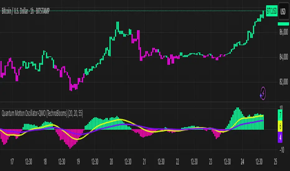
Quantum Motion Oscillator-QMO (TechnoBlooms)Quantum Motion Oscillator (QMO) is a momentum indicator designed for traders who demand precision. Combining multi-timeframe weighted linear regression with EMA crossovers, QMO offers a dynamic view of market momentum, helping traders anticipate trend shifts with greater accuracy.
This oscillator is inspired by quantum mechanics and wave theory, where market movement is seen as a series of probabilistic waves rather than rigid structures.
The histogram is plotted in proportion to the price movement of the candlesticks.
KEY FEATURES
1. Multi-Timeframe Histogram - Integrates 1 to 5 weighted linear regression averages, reducing lag while maintaining accuracy.
2. EMA Crossover Signal - Uses a Short and Long EMA to confirm trend shifts with minimal noise.
3. Adaptive Trend Analysis - Self-adjusting mechanics make QMO effective in both ranging and trending markets.
4. Scalable for Different Trading Styles - Works seamlessly for scalping, intraday, swing and position trading.
ADVANCED PROFESSIONAL INSIGHTS
1. Wave Dynamics and Market Flow - Inspired by wave mechanics, QMO reflects the energy accumulation and dissipation in price movements.
Expanding histogram waves = Strong momentum surge
Contracting waves = Momentum weakening, potential reversal zone.
2. Liquidity and Order Flow Applications - QMO works well alongside liquidity concepts and smart money techniques:
Combine with Fair Value Gaps & Order Blocks -> Enter when QMO signals align with liquidity zones.
Avoid False Moves - If price sweeps liquidity, but QMO momentum diverges, it is a sign of potential smart money manipulation.
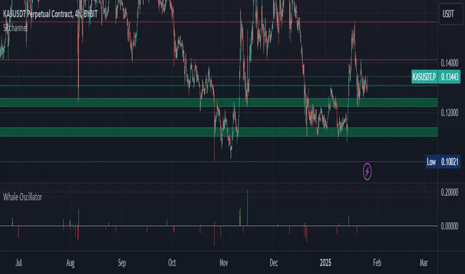
Whale Activity Impact OscillatorThe "Whale Activity Impact Oscillator" is a Pine Script v6 component designed to identify abnormal price movements caused by potential whale activity in the crypto market.
Here's how it works:
Inputs: The script allows users to configure the volume spike multiplier, price spike multiplier, lookback period, minimum volume threshold, and thresholds for strong buy and sell signals.
Data Calculations: It calculates the average volume and average percentage price change over the specified lookback period.
Whale Detection Logic: The script detects a volume spike if the current volume exceeds the average volume by the specified multiplier. It detects a price spike if the percentage price change exceeds the average by the specified multiplier.
Signals: A buy signal is generated when both a volume spike and a price increase are detected. A sell signal is generated when both a volume spike and a price decrease are detected.
Output: The oscillator is displayed as a histogram below the price chart. Green bars indicate buy signals, red bars indicate sell signals, and gray bars indicate normal activity. The height of the bars is proportional to the magnitude of the price change.
Alerts: The script includes alerts for whale buying and selling detected signals.
Edge Cases: The script avoids false signals in low-liquidity environments by setting a minimum volume threshold and filtering out signals during low market activity.
This component can be added to a TradingView chart to help traders identify potential whale activity and make informed trading decisions.
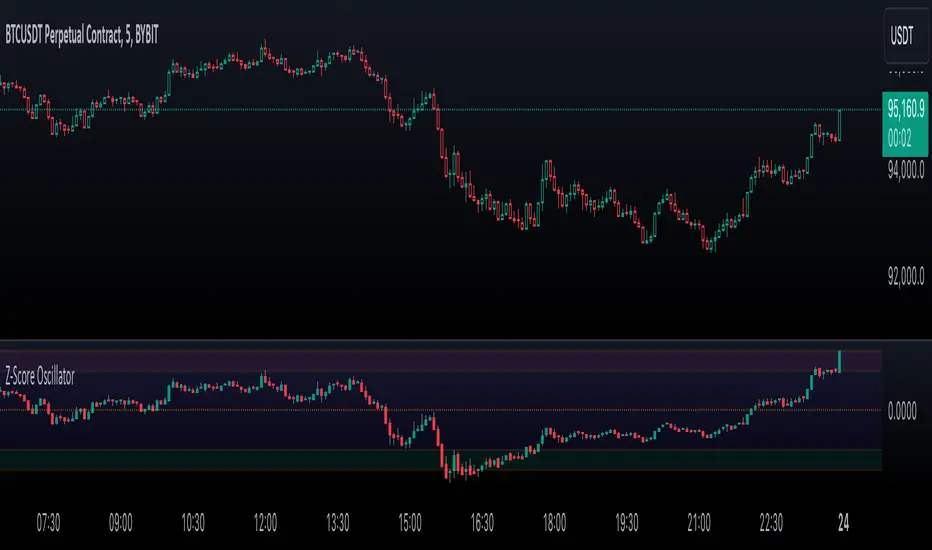
Enhanced Price Z-Score OscillatorThe Enhanced Price Z-Score Oscillator by tkarolak is a powerful tool that transforms raw price data into an easy-to-understand statistical visualization using Z-Score-derived candlesticks. Simply put, it shows how far prices stray from their average in terms of standard deviations (Z-Scores), helping traders identify when prices are unusually high (overbought) or unusually low (oversold).
The indicator’s default feature displays Z-Score Candlesticks, where each candle reflects the statistical “distance” of the open, high, low, and close prices from their average. This creates a visual map of market extremes and potential reversal points. For added flexibility, you can also switch to Z-Score line plots based on either Close prices or OHLC4 averages.
With clear threshold lines (±2σ and ±3σ) marking moderate and extreme price deviations, and color-coded zones to highlight overbought and oversold areas, the oscillator simplifies complex statistical concepts into actionable trading insights.
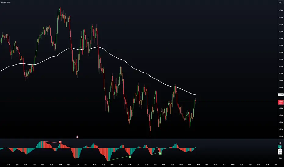
Awesome Oscillator with DivergenceSimple Awesome Oscillator with Divergences
This TradingView script combines the classic Awesome Oscillator (AO) with divergence detection. It plots AO as a histogram, highlighting changes in momentum. Divergences are identified based on pivot highs and lows, signaling potential trend reversals:
- Bullish Divergence: Price makes lower lows, AO makes higher lows.
- Bearish Divergence: Price makes higher highs, AO makes lower highs.
Visual signals (arrows) and alerts ensure clear identification, making it ideal for traders focusing on momentum and trend reversals.
Stablecoin Dominance Oscillator
The SDO is a normalized oscillator that tracks the relationship between stablecoin market capitalization (USDT + USDC + DAI) and total crypto market capitalization. It helps identify periods where stablecoins represent an unusually high or low portion of the total crypto market value.
Key components:
Main Signal (Blue Line):
Shows the normalized deviation of stablecoin dominance from its trend. Higher values indicate higher stablecoin dominance relative to history (which often corresponds with market bottoms/fear), while lower values indicate lower stablecoin dominance (often seen during strong bull markets/greed).
Dynamic Bands (Gray):
These adapt to market volatility, expanding during volatile periods and contracting during stable periods
Generally suggest temporary boundaries for the oscillator
Volatility Reference (Purple Line):
Shows the ratio between short-term and long-term volatility
Higher values indicate more volatile market conditions
Helps contextualize the reliability of the current signal
The indicator uses a 500-period lookback for baseline calculations and a 15-period Hull Moving Average for smoothing, making it responsive while filtering out noise. The final signal is normalized and volatility-adjusted to maintain consistent readings across different market regimes.

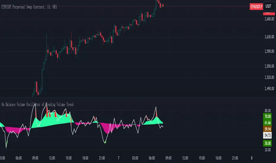
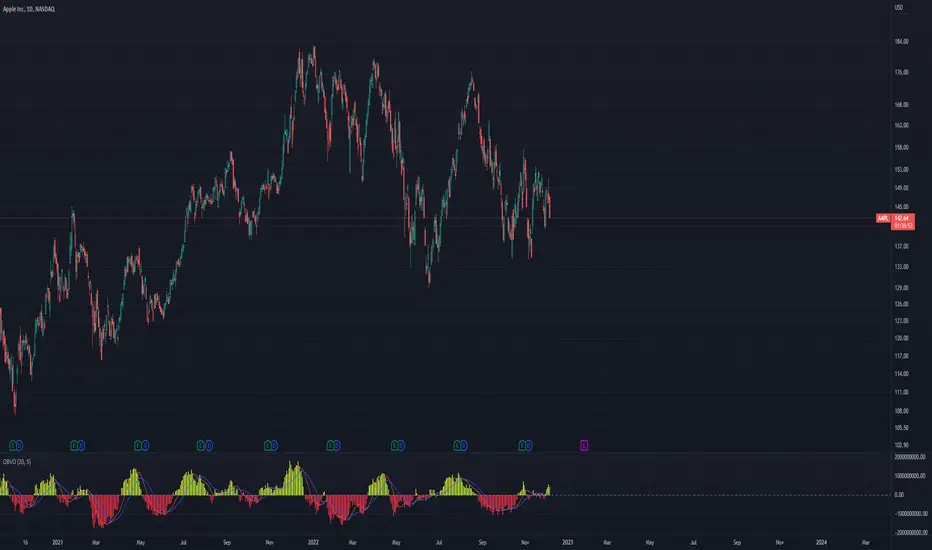
On Balance Volume Oscillator of Trading Volume TrendOn Balance Volume Oscillator of Trading Volume Trend
Introduction
This indicator, the "On Balance Volume Oscillator of Trading Volume Trend," is a technical analysis tool designed to provide insights into market momentum and potential trend reversals by combining the On Balance Volume (OBV) and Relative Strength Index (RSI) indicators.
Calculation and Methodology
* OBV Calculation: The indicator first calculates the On Balance Volume, which is a cumulative total of the volume of up days minus the volume of down days. This provides a running tally of buying and selling pressure.
* RSI of OBV: The RSI is then applied to the OBV values to smooth the data and identify overbought or oversold conditions.
* Exponential Moving Averages (EMAs): Two EMAs are calculated on the RSI of OBV. A shorter-term EMA (9-period in this case) and a longer-term EMA (100-period) are used to generate signals.
Interpretation and Usage
* EMA Crossovers: When the shorter-term EMA crosses above the longer-term EMA, it suggests increasing bullish momentum. Conversely, a downward crossover indicates weakening bullish momentum or increasing bearish pressure.
* RSI Divergences: Divergences between the price and the indicator can signal potential trend reversals. For example, if the price is making new highs but the indicator is failing to do so, it could be a bearish divergence.
* Overbought/Oversold Conditions: When the RSI of OBV is above 70, it suggests the market may be overbought and a potential correction could be imminent. Conversely, when it is below 30, it suggests the market may be oversold.
Visual Representation
The indicator is plotted on a chart with multiple lines and filled areas:
* Two EMAs: The shorter-term EMA and longer-term EMA are plotted to show the trend of the OBV.
* Filled Areas: The area between the two EMAs is filled with a color to indicate the strength of the trend. The color changes based on whether the shorter-term EMA is above or below the longer-term EMA.
* RSI Bands: Horizontal lines at 30 and 70 mark the overbought and oversold levels for the RSI of OBV.
Summary
The On Balance Volume Oscillator of Trading Volume Trend provides a comprehensive view of market momentum and can be a valuable tool for traders. By combining the OBV and RSI, this indicator helps identify potential trend reversals, overbought and oversold conditions, and the strength of the current trend.
Note: This indicator should be used in conjunction with other technical analysis tools and fundamental analysis to make informed trading decisions.
Awesome Oscillator + Bars count lines + EMA LineThe indicator includes an Awesome Oscillator with 2 vertical lines at a distance of 100 and 140 bars from the last bar to determine the third Elliott wave by the maximum peak of AO in the interval from 100 to 140 bars according to Bill Williams' Profitunity strategy. Additionally, a faster EMA line is displayed that calculates the difference between 5 Period and 34 Period Exponential Moving Averages (EMA 5 - EMA 34) based on the midpoints of the bars, just like AO calculates the difference between Simple Moving Averages (SMA 5 - SMA 34).
In the indicator settings, you can change the number of bars for vertical lines and any parameters for AO and EMA - method (SMA, Smoothed SMA, EMA and others), length, source (open, high, low, close, hl2 and others).
***
Индикатор включает Awesome Oscillator с 2 вертикальными линиями на расстоянии 100 и 140 баров от последнего бара, чтобы определить третью волну Эллиота по максимальному пику AO в интервале от 100 до 140 баров по стратегии Profitunity Билла Вильямса. Дополнительно отображается более быстрая линия EMA, которая вычисляет разницу между 5 Периодной и 34 Периодной Экспоненциальными Скользящими Средними (EMA 5 - EMA 34) по средним точкам баров (hl2), точно так же, как AO вычисляет разницу между Простыми Скользящими Средними (SMA 5 - SMA 34).
В настройках индикатора вы можете изменить количество баров для вертикальных линий и любые параметры для AO и EMA – метод (SMA, Smoothed SMA, EMA и другие), длину, источник (open, high, low, close, hl2 и другие).

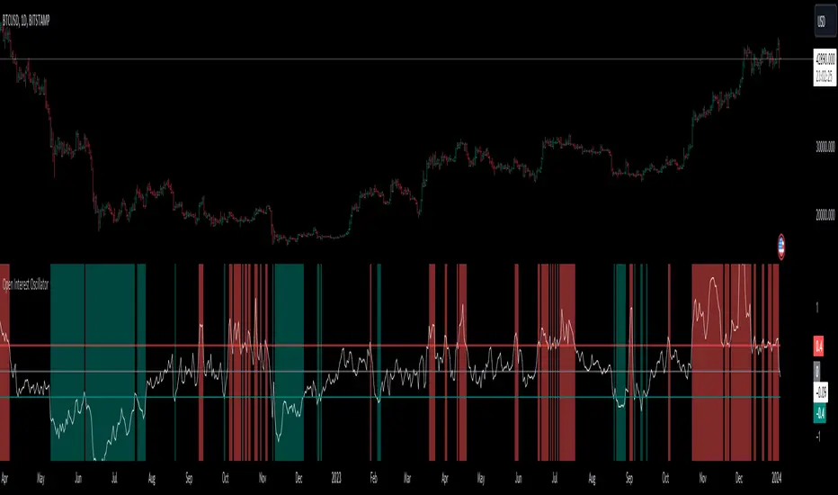
Open Interest OscillatorIn the middle of a bustling cryptocurrency market, with Bitcoin navigating a critical phase and the community hype over potential ETF approvals, current funding rates, and market leverage, the timing is optimal to harness the capabilities of sophisticated trading tools.
Meet the Open Interest Oscillator – special indicator tailored for the volatile arena of cryptocurrency trading. This powerful instrument is adept at consolidating open interest data from a multitude of exchanges, delivering an in-depth snapshot of market sentiment across all timeframes, be it a 1-minute sprint or a weekly timeframe.
This versatile indicator is compatible with nearly all cryptocurrency pairs, offering an expansive lens through which traders can gauge the market's pulse.
Key Features:
-- Multi-exchange Data Aggregation: This feature taps into the heart of the crypto market by aggregating open interest data from premier exchanges such as BINANCE, BITMEX, BITFINEX, and KRAKEN. It goes a step further by integrating data from various pairs and stablecoins, thus providing traders with a rich, multi-dimensional view of market activities.
-- Open Interest Bars: Witness the flow of market dynamics through bars that depict the volume of positions being opened or closed, offering a clear visual cue of trading behavior. In this mode, If bars are going into negative zone, then traders are closing their positions. If they go into positive territory - leveraged positions are being opened.
-- Bollinger Band Integration: Incorporate a layer of statistical analysis with standard deviation calculations, which frame the open interest changes, giving traders a quantified edge to evaluate the market's volatility and momentum.
-- Oscillator with Customizable Thresholds: Personalize your trading signals by setting thresholds that resonate with your unique trading tactics. This customization brings the power of tailored analytics to your strategic arsenal.
-- Max OI Ceiling Setting: In the fast-paced crypto environment where data can surge to overwhelming levels, the Max OI Ceiling ensures you maintain a clear view by capping the open interest data, thus preserving the readability and interpretability of information, even when market activity reaches feverish heights.
Advanced Volatility Oscillator with SignalsTitle: Advanced Volatility Oscillator with Signals (AVO-S)
In-Depth Description:
Introduction:
The Advanced Volatility Oscillator with Signals (AVO-S) is designed to offer traders a nuanced understanding of market volatility, combining traditional concepts with innovative visual aids and signal interpretation. This indicator is tailored for diverse financial markets, helping to identify potential trend reversals and momentum shifts.
Calculation and Methodology:
Spike Calculation: The core of AVO-S is the 'spike', calculated as the difference between the closing and opening prices (spike = close - open). This measure provides a straightforward gauge of intra-period volatility.
Standard Deviation: The indicator employs standard deviation to assess the variability of the 'spike', offering a dynamic threshold for understanding market extremities (stdDev = stdev(spike, length)).
Colored Columns: These columns visually represent the 'spike'. Their color changes based on the spike’s value relative to the zero line and the standard deviation threshold, providing an immediate visual cue of market state.
Blue Columns: Indicate moderate positive movement when the spike is above zero but below the standard deviation.
Green and Red Columns: Suggest stronger bullish (above standard deviation) and bearish (below negative standard deviation) movements, respectively.
Bullish and Bearish Signals:
The indicator generates signals based on the relationship between the 'spike' and its standard deviation.
Bullish Signals: Shown as upward triangles, these are formed when the 'spike' crosses above the standard deviation, indicating potential upward momentum.
Bearish Signals: Represented by downward triangles, these signals are generated when the 'spike' falls below the negative standard deviation, hinting at potential downward trends.
Usage and Application:
Traders can use the colored columns to quickly assess market sentiment and volatility.
The bullish and bearish signals serve as potential indicators for market entry or exit points, or for further analysis in conjunction with other technical tools.
Inspiration and Credits:
Inspired by Veryfid's original Volatility Oscillator, the AVO-S refines and builds upon these ideas to provide a comprehensive and user-friendly tool for market analysis. This indicator is a testament to the continuous evolution of technical analysis tools in the trading community.

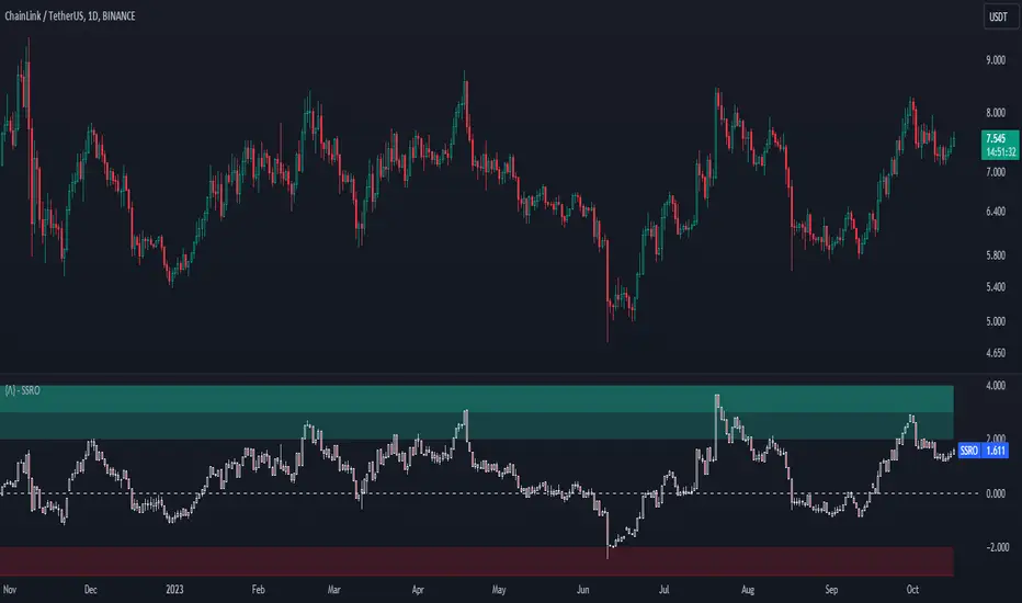
Stablecoin Supply Ratio Oscillator
The Stablecoin Supply Ratio Oscillator (SSRO) is a cryptocurrency indicator designed for mean reversion analysis and sentiment assessment. It calculates the ratio of CRYPTO:BTCUSD 's market capitalization to the sum of stablecoins' market capitalization and z-scores the result, offering insights into market sentiment and potential turning points.
Methodology:
The SSRO is calculated as follows-
method ssro(float src, array stblsrc, int len) =>
float ssr = src / stblsrc.sum() // Source of the underlying divided by the sum of stablecoin sources
(ssr - ta.sma(ssr, len)) / ta.stdev(ssr, len) // Z-Score Transformed
This ratio is Z-Scored to provide a standardized measure, allowing users to identify periods of market fear or greed based on the allocation of capital between the underlying and Stablecoins ( CRYPTOCAP:USDT , CRYPTOCAP:USDC , CRYPTO:TUSD , CRYPTOCAP:BUSD , CRYPTOCAP:DAI , CRYPTOCAP:USDD , CRYPTOCAP:FRAX ). The z-scored values indicate potential areas of discount (buying opportunities) or premium (selling opportunities) relative to historical patterns.
Customization:
Underlying Asset: SSRO is customizable to different underlying assets, offering a versatile tool for various cryptocurrencies.
Calculation Length: Users can adjust the length of the calculation, tailoring the indicator to short or long-term analysis.
Visualization: SSRO can be displayed as candles, providing a visual representation of premium and discount areas.
Interpretation:
Market Sentiment: Lower SSRO values may indicate market fear, suggesting a preference for stablecoins as a relatively safer haven for capital. Conversely, higher values may suggest market greed, as more capital is allocated to the underlying asset.
Utility and Use Cases:
1. Mean Reversion Analysis: SSRO identifies potential mean reversion opportunities, guiding traders on optimal entry and exit points.
2. Sentiment Analysis: The indicator provides insights into market sentiment, aiding traders in understanding market dynamics.
3. Macro Analysis: The majority of cryptos follow \ correlate to CRYPTO:BTCUSD , Therefore by assessing premium and discount areas of CRYPTO:BTCUSD relative to the chosen underlying asset, users gain insights into potential market tops and bottoms.
4. Divergence Analysis: SSRO divergence from price trends can signal potential reversals, providing traders with additional confirmation for their decisions.
The Stablecoin Supply Ratio Oscillator is a valuable tool for cryptocurrency traders, offering a nuanced perspective on market sentiment and mean reversion opportunities. Its customization options and visual representation make it a versatile and powerful addition to the crypto analyst's toolkit.
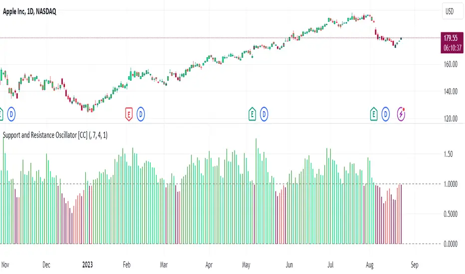
Support and Resistance Oscillator [CC]The Support and Resistance Oscillator is an experimental script I created to identify when the current price breaks a support or resistance line and reflect this value in an oscillator formula. This indicator uses a threshold to decide the dividing line between buying and selling points. Feel free to change the threshold or smoothing settings to see if you find anything better since this is so experimental. I'm double smoothing the difference between the indicator and its signal line to attempt to capture a combo of the price momentum combined with the general support and resistance levels. I have used dark colors for strong signals and lighter colors for normal signals and make sure to buy when the line turns green and sell when it turns red.
Let me know if there are any other scripts or indicators you would like to see me publish!
EMA X Oscillator
This indicator combines elements of the Exponential Moving Average (EMA) crossover and Rate of Change (ROC), generating a solid simple tool for technical analysis.
Overall, this script creates an oscillator by calculating the Rate of Change between two Exponential Moving Averages (Fast and Slow) based on the chosen smoothing methods and lengths. The oscillator helps identify potential trends. It offers customization options for the types of smoothing and other parameters, making it versatile for various strategies.

Momentum Covariance Oscillator by TenozenWell, guess what? A new indicator is here! Again it's a coincidence, as I experiment with my formula. So far it's less noisy than Autoregressive Covariance Oscillator, so possibly this one is better. The formula is much simpler, care me to explain.
___________________________________________________________________________________________________
Yt = close - previous average
Val = Yt/close
___________________________________________________________________________________________________
Welp that's the formula lol. Funny thing is that it's so simple, but it's good! What matters is the use of it haha.
So how to use this Oscillator? If the value is above 0, we expect a bullish response, if the value is below 0 we expect a bearish response. That simple. Ciao.
(Any questions and suggestions? feel free to comment!)

Autoregressive Covariance Oscillator by TenozenWell to be honest I don't know what to name this indicator lol. But anyway, here is my another original work! Gonna give some background of why I create this indicator, it's all pretty much a coincidence when I'm learning about time series analysis.
_ _ _ _ _ _ _ _ _ _ _ _ _ _ _ _ _ _ _ _ _ _ _ _ _ _ _ _ _ _ _ _ _ _ _ _ _
Well, the formula of Auto-covariance is:
E{(X(t)-(t) * (X(t-s)-(t-s))}= Y_s
But I don't multiply both values but rather subtract them:
E{(X(t)-(t) - (X(t-s)-(t-s))}= Y_s?
_ _ _ _ _ _ _ _ _ _ _ _ _ _ _ _ _ _ _ _ _ _ _ _ _ _ _ _ _ _ _ _ _ _ _ _ _
For arm_vald, the equation is as follows:
arm_vald = val_mu + mu_plus_lsm + et
val_mu --> mean of time series
mu_plus_lsm --> val_mu + LSM
et --> error term
As you can see, val_mu^2. I did this so the oscillator is much smoother.
_ _ _ _ _ _ _ _ _ _ _ _ _ _ _ _ _ _ _ _ _ _ _ _ _ _ _ _ _ _ _ _ _ _ _ _ _
After I get the value, I normalize them:
aco = Y_s? / arm_vald
So by this calculation, I get something like an oscillator!
(more details in the code)
_ _ _ _ _ _ _ _ _ _ _ _ _ _ _ _ _ _ _ _ _ _ _ _ _ _ _ _ _ _ _ _ _ _ _ _ _
So how to use this indicator? It's so easy! If the value is above 0, we gonna expect a bullish response, if the value is below 0, we gonna expect a bearish response; that simple. Be aware that you should wait for the price to be closed before executing a trade.
Well, try it out! So far this is the most powerful indicator that I've created, hope it's useful. Ciao.
(more updates for the indicator if needed)

Faytterro Oscillatorwhat is Faytterro oscillator?
An oscillator that perfectly identifies overbought and oversold zones.
what it does?
this places the price between 0 and 100 perfectly but with a little delay. To eliminate this delay, it predicts the price to come, and the indicator becomes clearer as the probability of its prediction increases.
how it does it?
This indicator is obtained with "faytterro bands", another indicator I designed. For more information about faytterro bands:
A kind of stochastic function is applied to the faytterro bands indicator, and then another transformation formula that I have designed and explained in detail in the link above is applied. These formulas are also applied again to calculate the prediction parts.
how to use it?
Use this indicator to see past overbought and oversold zones and to see future ones.
The input named source is used to change the source of the indicator.
The length serves to change the signal frequency of the indicator.

Custom OBV OscillatorThis is a modified OBV indicator that creates an oscillator by smoothing the difference between the value of the OBV and a short moving average of the OBV. SMAs of the oscillator are also provided to study crosses and convergence/divergence.
The indicator should mostly be used on common stock, but works on futures contracts with some tuning and a shorter timeframe.
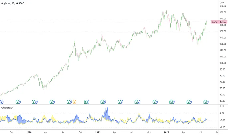
Whisker Reversal Oscillator [SpiritualHealer117]The Whisker Reversal Oscillator can be used to spot strength or weakness in trends. It is designed for stocks, commodities and forex trading, and is intended to be calculated from the high, close, low, and open over a given length.
Features:
The Whisker Reversal Oscillator shows the average length of the top and bottom whiskers on candlesticks over a defined length. It plots the percentage difference between the whiskers and the length of the body, with the yellow line representing the average length of the top whisker, and the bottom line indicating the average length of the bottom whisker.
Interpreting the signals:
The Whisker Reversal Oscillator is interpreted in the same way as a candlestick reversal pattern, where it being bullish or bearish depends on the trend. In a bull trend, if the yellow line passes above the blue line, it means the top whiskers are longer on average than the bottom whiskers, which may show that bulls were too weak to hold a rally, and signal a reversal. On the other hand, in a bear trend, if the yellow line is above the blue line, it indicates that the bulls were able to push the price up, which would be bullish. If the blue line crosses over the yellow line in an uptrend, it's often a bearish sign, but if it happens in a downtrend, its a bullish sign.
Generally speaking, a cross in the lines is indicative of a potential reversal, and when the lines cross over 1, it means that the whiskers were bigger than the candlestick bodies over your selected length, indicating that a big swing will come.
Smoothed RSI Heikin Ashi Oscillator w/ Expanded Types [Loxx]Smoothed RSI Heikin-Ashi Oscillator w/ Expanded Types is a spin on Heikin Ashi RSI Oscillator by @JayRogers. The purpose of this modification is to reduce noise in the original version thereby increasing suitability of the signal output. This indicator is tuned for Forex markets.
Differences:
35+ Smoothing Options for RSI
35+ Smoothing Options for HA Candles
Heiken-Ashi Better Expanded Source input. This source input is use for the RSI calculation only.
Signals
Alerts
What are Heiken-Ashi "better" candles?
The "better formula" was proposed in an article/memo by BNP-Paribas (In Warrants & Zertifikate, No. 8, August 2004 (a monthly German magazine published by BNP Paribas, Frankfurt), there is an article by Sebastian Schmidt about further development (smoothing) of Heikin-Ashi chart.)
They proposed to use the following :
(Open+Close)/2+(((Close-Open)/( High-Low ))*ABS((Close-Open)/2))
instead of using :
haClose = (O+H+L+C)/4
According to that document the HA representation using their proposed formula is better than the traditional formula.
What are traditional Heiken-Ashi candles?
The Heikin-Ashi technique averages price data to create a Japanese candlestick chart that filters out market noise.
Heikin-Ashi charts, developed by Munehisa Homma in the 1700s, share some characteristics with standard candlestick charts but differ based on the values used to create each candle. Instead of using the open, high, low, and close like standard candlestick charts, the Heikin-Ashi technique uses a modified formula based on two-period averages. This gives the chart a smoother appearance, making it easier to spots trends and reversals, but also obscures gaps and some price data.
Future updates
Expand signal options to include RSI-, Zero-, and color-crosses

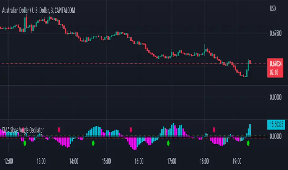
EMA Slope/Angle OscillatorEMA Slope/Angle Oscillator, Multiple Moving Average Oscillator, Multiple type
Moving Averages HMA,EMA,WMA,SMA, VWMA,VWAP provided.
The angle is calculated between the Slow MA and Fast MA and the difference between the angle is plotted as Histogram.
Additionally Buy Sell Signals are plotted as green and red Dots.
its very easy to judge the movement of price Bearish/Bullish.
Bearish if price below 0 line
Bullish if price above 0 line
Zero crossing is Moving Average Crossover.
Trend Filter is provided to filter opposite signals.
Angle Threshold is provided to filter low angle false signals.
Dead zone is plotted around Zero Line. Trades can be taken after Threshold angle or Dead zone is crossed
Its interesting to see how different Moving Averages move along with price Action.
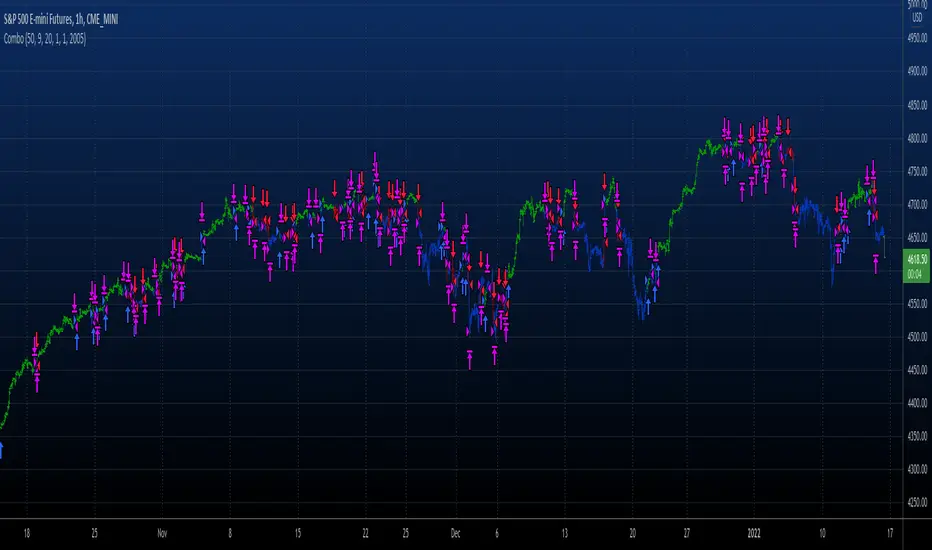
Combo 2/20 EMA & Absolute Price Oscillator (APO) This is combo strategies for get a cumulative signal.
First strategy
This indicator plots 2/20 exponential moving average. For the Mov
Avg X 2/20 Indicator, the EMA bar will be painted when the Alert criteria is met.
Second strategy
The Absolute Price Oscillator displays the difference between two exponential
moving averages of a security's price and is expressed as an absolute value.
How this indicator works
APO crossing above zero is considered bullish, while crossing below zero is bearish.
A positive indicator value indicates an upward movement, while negative readings
signal a downward trend.
Divergences form when a new high or low in price is not confirmed by the Absolute Price
Oscillator (APO). A bullish divergence forms when price make a lower low, but the APO
forms a higher low. This indicates less downward momentum that could foreshadow a bullish
reversal. A bearish divergence forms when price makes a higher high, but the APO forms a
lower high. This shows less upward momentum that could foreshadow a bearish reversal.
WARNING:
- For purpose educate only
- This script to change bars colors.
+ REX OscillatorSo, what is the REX oscillator, you might be asking yourself.
"The Rex oscillator is an indicator that measures market behavior based on the relationship of the close to the open, high and low values of the same bar. A big difference between the high and close on a bar indicates weakness, and wide disparity between the low and close indicates strength. The difference between open and close also indicates market performance."
The True Value of a Bar (TVB) gives an indication of how healthy the market is. A negative close and a positive TVB (or vice versa) is an indication of the market building strength on the opposing side of the trend. The Rex oscillator is a moving average of the TVB value with the specified period.
I first came across this watching one of many No Nonsense Forex videos. Mostly, from comments I've read, it is used as an exit indicator for people who trade with a system similar or identical to the one VP espouses in his NNFX blog. I think it's perfectly apt to use as an entry indicator as well, or even as both, perhaps, depending on the moving average you chose to apply to the TVB.
There are a few other versions of this on tradingview, but I thought I'd make an updated version. Added Donchian Channels because I like the idea of a dynamic sort of overbought/sold area. I left out the basis because the indicator pivots around a center line, and has a signal line as well. A basis line just seemed like too much, and would likely not be very useful.
The additional usual things that I incorporate into my indicators are included here: optional candle coloring, alerts, and probably a too large selection of moving averages.
Credit to Nemozny for the FRAMA calculation. I may add that to other indicators I have.
