VWAP Multi Sessions + EMA + TEMA + PivotThis indicator combines several technical tools in one, designed for both intraday and swing traders to provide a complete view of market dynamics.
- VWAP Multi Sessions: calculates and plots five independent VWAPs, each based on a specific time range. This allows you to better identify value zones and price evolution during different phases of the trading day.
- Moving Averages (EMA): three strategic EMAs (55, 144, and 233 periods) are included to track the broader trend and highlight potential crossovers.
- TEMA (Triple Exponential Moving Average): two TEMAs (144 and 233 periods) offer a more responsive alternative to EMAs, reducing lag while filtering out some market noise.
- Daily Levels: the previous day’s open, close, high, and low are plotted as key support and resistance references.
- Pivot Point (P): also included is the classic daily pivot from the previous session, calculated as (High + Low + Close) / 3, which acts as a central level around which price often gravitates.
In summary, this indicator combines:
- intraday value references (session VWAPs),
- trend indicators (EMA and TEMA),
- and daily reference points (OHLC and Pivot).
It is particularly suited for intraday, scalping, and swing trading strategies, helping traders anticipate potential reaction zones in the market more effectively.
Search in scripts for "纳斯达克指数期货cfd"

Exhaustion Detector by exp3rtsThis advanced indicator is designed to spot buyer and seller exhaustion zones by combining candle structure, volume anomalies, momentum oscillators, and support/resistance context. Optimized for the 5-minute chart, it highlights potential turning points where momentum is likely fading.
Multi-factor detection – Uses RSI, Stochastic, volume spikes, wick-to-body ratios, and ATR context to identify exhaustion.
Smart filtering – Optional trend filter (EMA) and support/resistance proximity filter refine signals.
Cooldown logic – Prevents repeated signals in rapid succession to reduce noise.
Confidence scoring – Each exhaustion signal is graded for strength, so you can gauge conviction.
Visual clarity – Clear arrows mark exhaustion signals, background zones highlight pressure areas, and debug labels show score breakdowns (toggleable).
Use this tool to:
Anticipate potential reversals before price turns
Spot exhaustion at key support/resistance zones
Add a contrarian signal filter to your trading system

Nth Candle by exp3rtsThis lightweight and versatile TradingView indicator highlights every Xth candle on your chart, making it easy to spot cyclical price behavior or track specific intervals in the market.
- Custom Interval – Choose how often candles should be highlighted (e.g., every 5th, 10th, or
20th bar).
- Color Coding – Highlighted candles are shaded green if bullish and red if bearish, giving you
quick visual insights into momentum at those intervals.
- Clean Overlay – The indicator draws directly on your main chart without clutter, so you can
combine it with your favorite setups and strategies.
Use this tool to:
1) Identify repeating patterns and cycles
2) Mark periodic reference candles
3) Support discretionary trading decisions with clear visual cues

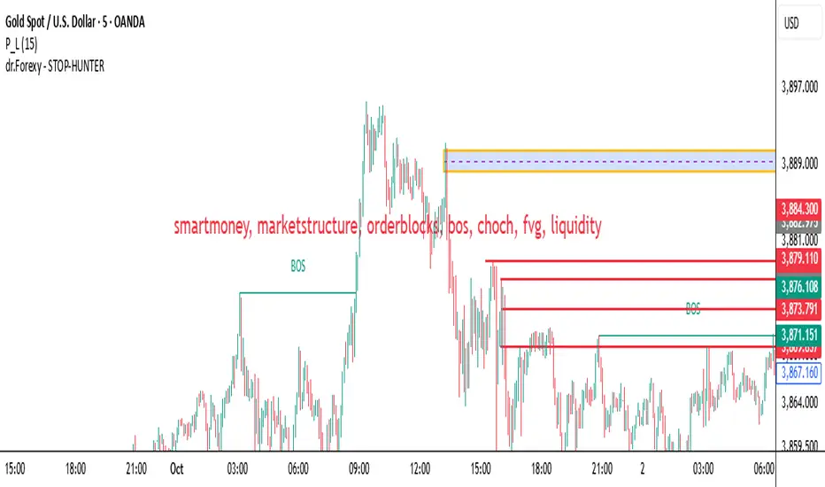
HUNT_line [Dr.Forexy]HUNT_line Indicator
📊 **Category:** Price Action & Market Structure
⏰ **Recommended Timeframe:** 5-minute and higher
🎯 **Purpose:** Advanced market structure visualization for professional traders
⸻
⚡ **Key Features:**
• Break of Structure (BOS) and Change of Character (CHOCH) detection
• Internal & Swing Market Structure analysis
• Order Blocks identification with smart filtering
• Fair Value Gaps (FVG) visualization
• Premium/Discount Zones
• Multi-timeframe support
• Real-time structure alerts
⸻
🛠 **How to Use:**
1. Apply on 5M or higher timeframes for best results
2. Monitor BOS/CHOCH for trend direction changes
3. Use Order Blocks as potential support/resistance areas
4. Watch for FVG fills as price inefficiency zones
5. Combine multiple confluences for higher probability setups
⸻
⚠️ **Risk Disclaimer:**
This indicator is for educational purposes only.
Not financial advice. Always conduct your own research.
⸻
🔹 **Credits:**
Inspired by LuxAlgo's "Smart Money Concepts" with custom improvements
EMA CloudThe EMA Crossover Cloud is a clean and intuitive indicator that combines two Exponential Moving Averages (EMA) into a visual cloud.
Key features:
Cloud visualization: The space between EMA A and EMA B is shaded, making the current trend direction easier to identify.
Crossover signals: A clear LONG signal is plotted when EMA A crosses above EMA B, and a SHORT signal when EMA A crosses below EMA B.
Bar coloring: Candles are automatically colored according to the trend (uptrend, downtrend, or neutral).
Customizable colors: Cloud, signals, and bars can all be customized to match your chart style.
Alerts ready: Built-in alerts for EMA crossovers (LONG/SHORT).
Status label: A compact label shows the current cloud trend state in real time.
This indicator is ideal for traders who prefer simple and reliable crossover signals combined with a clear trend visualization. It works on any timeframe or asset.

Engulfing Pattern Scanner with RSI FilterEngulfing Pattern Scanner with RSI Filter
This indicator identifies high-probability engulfing patterns using multiple confirmation filters including candle stability, RSI divergence, and price momentum over a specified period.
═══ INDICATOR LOGIC ═══
BUY Signal Generated When:
• Bullish engulfing pattern forms
• Candle stability exceeds threshold (body/wick ratio)
• RSI is below oversold threshold
• Price has decreased over the delta period
• Bar is confirmed (no repainting)
SELL Signal Generated When:
• Bearish engulfing pattern forms
• Candle stability exceeds threshold
• RSI is above overbought threshold
• Price has increased over the delta period
• Bar is confirmed (no repainting)
═══ KEY FEATURES ═══
• Candle Stability Index (0-1): Filters out unstable/noisy candles
• RSI Index (0-100): Confirms momentum conditions
• Candle Delta Length: Defines lookback period for price movement
• Disable Repeating Signals: Removes consecutive same-direction signals
• Multiple visual styles: Text bubbles, triangles, or arrows
• Customizable colors and label sizes
• Built-in alert conditions
═══ INPUT PARAMETERS ═══
Candle Stability Index (0.5 default): Higher values require more decisive candles
RSI Index (50 default): Threshold for overbought/oversold conditions
Candle Delta Length (5 default): Bars to measure price change
Label customization: Size, style, and colors
═══ HOW TO USE ═══
1. Add indicator to chart
2. Adjust technical parameters based on market volatility
3. Set visual preferences for signal display
4. Create alerts using the built-in conditions
5. Higher Candle Stability = fewer but higher quality signals
6. Lower RSI Index = more conservative entry points
═══ BEST PRACTICES ═══
• Use on higher timeframes (4H+) for swing trading
• Combine with support/resistance for confluence
• Test parameters on historical data before live trading
• Consider market conditions when adjusting filters
═══ VERSION INFO ═══
Pine Script: v5
Repainting: No (uses barstate.isconfirmed)
Max Labels: 500
```

90min + Daily + Weekly Cycles + Alerts [Final]Quarterly theory indicator
Customizable indicator 90m cycles, daily, and weekly

aaa sibilio 5.5 New 4## **The Fundamental Characteristics of Moving Averages: Theoretical Principles and Strategic Applications**
### **The Non-Parallelism Principle: Mathematical Foundation**
The first fundamental principle governing moving averages establishes that **any moving average can never be parallel to its linear regression**. This is not coincidental or anomalous, but a direct consequence of the mathematical nature of moving averages.
**Theoretical explanation:** A moving average is a low-pass filter that removes high-frequency components from price data, while a linear regression represents the optimal linear trend over the considered period. Since the moving average maintains trace of oscillations around the trend (albeit attenuated), while the regression completely eliminates these oscillations to provide only the general direction, the two curves can never be identical or parallel.
**Crucial implication:** This characteristic certifies that **moving averages always have a curvilinear pattern** relative to their regression. The curvature is not an imperfection in the calculation, but the manifestation of the intrinsic dynamics of market data filtered through the moving average.
### **System Energy: Derivation from Curvature**
It is precisely this curvilinear characteristic that allows us to determine fundamental parameters such as **system energy**.
**Physical basis:** In physics, the potential energy of a curvilinear system is proportional to the deviation from the equilibrium trajectory (represented by the linear regression). In our context:
- **Potential energy** = Distance between moving average and its regression
- **Kinetic energy** = Speed of approach or separation between the two curves
- **Total system energy** = Sum of potential and kinetic energy
**Practical application:** When the moving average moves away from its regression, it accumulates potential energy that must be released. When it approaches rapidly, it manifests kinetic energy that can lead to overshooting the equilibrium point.
### **The Hierarchical Rolling Principle**
The second fundamental principle establishes that **curves roll around each other starting from longer periods toward shorter ones**. This phenomenon has deep roots in dynamical systems theory.
**Theoretical explanation:** Moving averages with longer periods have greater inertia and resistance to change (analogous to mass in physics). When a trend change occurs, it propagates first in long-period averages (which represent the dominant forces of the system), then progressively diffuses toward shorter-period averages.
**Propagation mechanism:**
1. **Macro level** (long averages): Change in direction of principal forces
2. **Medium level** (intermediate averages): Signal transmission
3. **Micro level** (short averages): Final manifestation of the change
### **Derived Strategic Formations**
This hierarchical rolling allows us to identify **important formations** for the strategy:
**Rolling Confluence:** When multiple averages of different periods simultaneously begin the rolling process, a high-probability reversal zone is created.
**Alignment Cascade:** The temporal sequence with which averages roll provides information about the strength and persistence of the imminent movement.
**Dynamic Resistance Zones:** Points where rolling encounters resistance indicate critical levels where opposing forces temporarily balance.
### **Strategic Implications**
These theoretical principles translate into concrete operational advantages:
1. **Energy predictability:** We can quantify the energy accumulated in the system and predict the strength of future movements
2. **Entry timing:** Hierarchical rolling provides a temporal sequence to optimize entry points
3. **Risk management:** Understanding system energy allows proper position sizing
The combination of these two principles - non-parallelism and hierarchical rolling - transforms moving averages from simple trend indicators into sophisticated tools for energetic and dynamic analysis of financial markets.

aaa sibilio 5.5 New Tre## **The Fundamental Characteristics of Moving Averages: Theoretical Principles and Strategic Applications**
### **The Non-Parallelism Principle: Mathematical Foundation**
The first fundamental principle governing moving averages establishes that **any moving average can never be parallel to its linear regression**. This is not coincidental or anomalous, but a direct consequence of the mathematical nature of moving averages.
**Theoretical explanation:** A moving average is a low-pass filter that removes high-frequency components from price data, while a linear regression represents the optimal linear trend over the considered period. Since the moving average maintains trace of oscillations around the trend (albeit attenuated), while the regression completely eliminates these oscillations to provide only the general direction, the two curves can never be identical or parallel.
**Crucial implication:** This characteristic certifies that **moving averages always have a curvilinear pattern** relative to their regression. The curvature is not an imperfection in the calculation, but the manifestation of the intrinsic dynamics of market data filtered through the moving average.
### **System Energy: Derivation from Curvature**
It is precisely this curvilinear characteristic that allows us to determine fundamental parameters such as **system energy**.
**Physical basis:** In physics, the potential energy of a curvilinear system is proportional to the deviation from the equilibrium trajectory (represented by the linear regression). In our context:
- **Potential energy** = Distance between moving average and its regression
- **Kinetic energy** = Speed of approach or separation between the two curves
- **Total system energy** = Sum of potential and kinetic energy
**Practical application:** When the moving average moves away from its regression, it accumulates potential energy that must be released. When it approaches rapidly, it manifests kinetic energy that can lead to overshooting the equilibrium point.
### **The Hierarchical Rolling Principle**
The second fundamental principle establishes that **curves roll around each other starting from longer periods toward shorter ones**. This phenomenon has deep roots in dynamical systems theory.
**Theoretical explanation:** Moving averages with longer periods have greater inertia and resistance to change (analogous to mass in physics). When a trend change occurs, it propagates first in long-period averages (which represent the dominant forces of the system), then progressively diffuses toward shorter-period averages.
**Propagation mechanism:**
1. **Macro level** (long averages): Change in direction of principal forces
2. **Medium level** (intermediate averages): Signal transmission
3. **Micro level** (short averages): Final manifestation of the change
### **Derived Strategic Formations**
This hierarchical rolling allows us to identify **important formations** for the strategy:
**Rolling Confluence:** When multiple averages of different periods simultaneously begin the rolling process, a high-probability reversal zone is created.
**Alignment Cascade:** The temporal sequence with which averages roll provides information about the strength and persistence of the imminent movement.
**Dynamic Resistance Zones:** Points where rolling encounters resistance indicate critical levels where opposing forces temporarily balance.
### **Strategic Implications**
These theoretical principles translate into concrete operational advantages:
1. **Energy predictability:** We can quantify the energy accumulated in the system and predict the strength of future movements
2. **Entry timing:** Hierarchical rolling provides a temporal sequence to optimize entry points
3. **Risk management:** Understanding system energy allows proper position sizing
The combination of these two principles - non-parallelism and hierarchical rolling - transforms moving averages from simple trend indicators into sophisticated tools for energetic and dynamic analysis of financial markets.

aaa sibilio 5.5 New Due## **Le Caratteristiche Fondamentali delle Medie: Principi Teorici e Applicazioni Strategiche**
### **Il Principio della Non-Parallelità: Fondamento Matematico**
Il primo principio fondamentale che governa le medie mobili stabilisce che **qualsiasi media non può mai essere parallela alla sua regressione lineare**. Questo non è un caso o un'anomalia, ma una conseguenza diretta della natura matematica delle medie mobili.
**Spiegazione teorica:** Una media mobile è un filtro passa-basso che rimuove le frequenze ad alta velocità dai dati di prezzo, mentre una regressione lineare rappresenta la tendenza lineare ottimale nel periodo considerato. Poiché la media mobile mantiene traccia delle oscillazioni attorno al trend (seppur attenuate), mentre la regressione elimina completamente queste oscillazioni per fornire solo la direzione generale, le due curve non possono mai essere identiche o parallele.
**Implicazione cruciale:** Questa caratteristica certifica che **le medie hanno sempre un andamento curvilineo** rispetto alla loro regressione. La curvatura non è un'imperfezione del calcolo, ma la manifestazione della dinamica intrinseca dei dati di mercato filtrati attraverso la media mobile.
### **L'Energia del Sistema: Derivazione dalla Curvatura**
È proprio questa caratteristica curvilinea che ci consente di determinare parametri fondamentali come **l'energia del sistema**.
**Base fisica:** In fisica, l'energia potenziale di un sistema curvilineo è proporzionale alla deviazione dalla traiettoria di equilibrio (rappresentata dalla regressione lineare). Nel nostro contesto:
- **Energia potenziale** = Distanza tra media mobile e sua regressione
- **Energia cinetica** = Velocità di avvicinamento o allontanamento tra le due curve
- **Energia totale del sistema** = Somma di energia potenziale e cinetica
**Applicazione pratica:** Quando la media si allontana dalla sua regressione, accumula energia potenziale che deve essere rilasciata. Quando si avvicina rapidamente, manifesta energia cinetica che può portare a overshooting del punto di equilibrio.
### **Il Principio dell'Arrotolamento Gerarchico**
Il secondo principio fondamentale stabilisce che **le curve si arrotolano tra loro partendo dai periodi più lunghi verso quelli più piccoli**. Questo fenomeno ha radici profonde nella teoria dei sistemi dinamici.
**Spiegazione teorica:** Le medie con periodi più lunghi hanno maggiore inerzia e resistenza al cambiamento (analogamente alla massa in fisica). Quando si verifica un cambiamento di tendenza, questo si propaga prima nelle medie a periodo lungo (che rappresentano le forze dominanti del sistema), per poi diffondersi progressivamente verso le medie a periodo più breve.
**Meccanismo di propagazione:**
1. **Livello macro** (medie lunghe): Cambio di direzione delle forze principali
2. **Livello medio** (medie intermedie): Trasmissione del segnale
3. **Livello micro** (medie brevi): Manifestazione finale del cambiamento
### **Formazioni Strategiche Derivate**
Questo arrotolamento gerarchico ci consente di identificare **formazioni importanti** per la strategia:
**Confluenza di Arrotolamento:** Quando più medie di diversi periodi iniziano simultaneamente il processo di arrotolamento, si crea una zona di alta probabilità di inversione.
**Cascata di Allineamento:** La sequenza temporale con cui le medie si arrotolano fornisce informazioni sulla forza e persistenza del movimento imminente.
**Zone di Resistenza Dinamica:** I punti dove l'arrotolamento incontra resistenza indicano livelli critici dove le forze opposte si equilibrano temporaneamente.
### **Implicazioni per la Strategia**
Questi principi teorici si traducono in vantaggi operativi concreti:
1. **Prevedibilità dell'energia:** Possiamo quantificare l'energia accumulata nel sistema e prevedere la forza dei movimenti futuri
2. **Timing degli ingressi:** L'arrotolamento gerarchico fornisce una sequenza temporale per ottimizzare i punti di ingresso
3. **Gestione del rischio:** La comprensione dell'energia del sistema permette di dimensionare correttamente le posizioni
La combinazione di questi due principi - non-parallelità e arrotolamento gerarchico - trasforma le medie mobili da semplici indicatori di trend in strumenti sofisticati per l'analisi energetica e dinamica dei mercati finanziari.
versione inglese
## **The Fundamental Characteristics of Moving Averages: Theoretical Principles and Strategic Applications**
### **The Non-Parallelism Principle: Mathematical Foundation**
The first fundamental principle governing moving averages establishes that **any moving average can never be parallel to its linear regression**. This is not coincidental or anomalous, but a direct consequence of the mathematical nature of moving averages.
**Theoretical explanation:** A moving average is a low-pass filter that removes high-frequency components from price data, while a linear regression represents the optimal linear trend over the considered period. Since the moving average maintains trace of oscillations around the trend (albeit attenuated), while the regression completely eliminates these oscillations to provide only the general direction, the two curves can never be identical or parallel.
**Crucial implication:** This characteristic certifies that **moving averages always have a curvilinear pattern** relative to their regression. The curvature is not an imperfection in the calculation, but the manifestation of the intrinsic dynamics of market data filtered through the moving average.
### **System Energy: Derivation from Curvature**
It is precisely this curvilinear characteristic that allows us to determine fundamental parameters such as **system energy**.
**Physical basis:** In physics, the potential energy of a curvilinear system is proportional to the deviation from the equilibrium trajectory (represented by the linear regression). In our context:
- **Potential energy** = Distance between moving average and its regression
- **Kinetic energy** = Speed of approach or separation between the two curves
- **Total system energy** = Sum of potential and kinetic energy
**Practical application:** When the moving average moves away from its regression, it accumulates potential energy that must be released. When it approaches rapidly, it manifests kinetic energy that can lead to overshooting the equilibrium point.
### **The Hierarchical Rolling Principle**
The second fundamental principle establishes that **curves roll around each other starting from longer periods toward shorter ones**. This phenomenon has deep roots in dynamical systems theory.
**Theoretical explanation:** Moving averages with longer periods have greater inertia and resistance to change (analogous to mass in physics). When a trend change occurs, it propagates first in long-period averages (which represent the dominant forces of the system), then progressively diffuses toward shorter-period averages.
**Propagation mechanism:**
1. **Macro level** (long averages): Change in direction of principal forces
2. **Medium level** (intermediate averages): Signal transmission
3. **Micro level** (short averages): Final manifestation of the change
### **Derived Strategic Formations**
This hierarchical rolling allows us to identify **important formations** for the strategy:
**Rolling Confluence:** When multiple averages of different periods simultaneously begin the rolling process, a high-probability reversal zone is created.
**Alignment Cascade:** The temporal sequence with which averages roll provides information about the strength and persistence of the imminent movement.
**Dynamic Resistance Zones:** Points where rolling encounters resistance indicate critical levels where opposing forces temporarily balance.
### **Strategic Implications**
These theoretical principles translate into concrete operational advantages:
1. **Energy predictability:** We can quantify the energy accumulated in the system and predict the strength of future movements
2. **Entry timing:** Hierarchical rolling provides a temporal sequence to optimize entry points
3. **Risk management:** Understanding system energy allows proper position sizing
The combination of these two principles - non-parallelism and hierarchical rolling - transforms moving averages from simple trend indicators into sophisticated tools for energetic and dynamic analysis of financial markets.

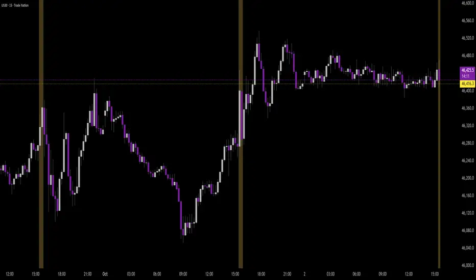
Time Range by exp3rtsTime Window highlights a custom time range directly on your chart, helping you focus on specific market sessions or trading hours.
Key Features:
Highlights a custom time range with a shaded background
Fully adjustable start and end time (hour & minute)
Supports multiple time zones (e.g., GMT, UTC, Europe/Berlin)
Optional market color shading inside the window (bull/bear neutral tone)
Use Cases:
Mark London Open, New York Session, or any session overlap
Focus on high-probability trading hours
Visualize your backtesting timeframe or algo activity window
Track premarket or after-hours activity for futures or indices
Customization:
Set the beginning and end time in your local or exchange time zone
Choose your timezone string (e.g., "GMT", "Etc/UTC", "America/New_York")
Automatically colors candles in the time window for easy visibility

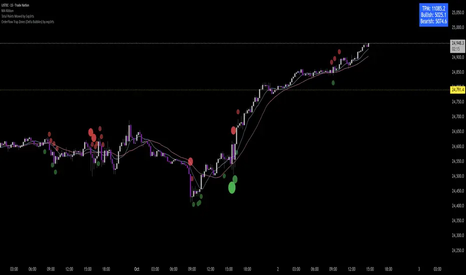
Total Points Moved by exp3rtsThis lightweight utility tracks the total intraday range of price movement, giving you real-time insight into market activity.
It calculates:
🟩 Bullish Points – Total range from bullish candles (close > open)
🟥 Bearish Points – Total range from bearish candles (close < open)
🔁 Total Points Moved (TPM) – Sum of all high–low ranges for the day
Values are pulled from the 1-second chart for high precision and displayed in a compact tag in the top-right corner.
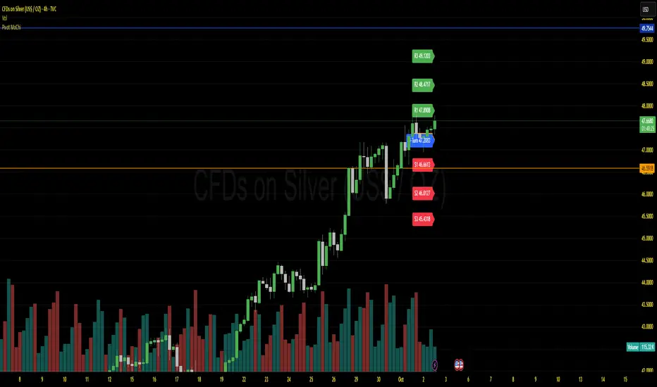
Pivot MoChiThis uses Current Day opening in place of previous day close
More Dynamic than Traditional Pivots
Cambio de Tendencia Multi-TF con PanelKey Features:
Functionalities:
4 Timeframes: 5 min, 15 min, 1 hour, and 4 hours
Visual dashboard with intuitive colors
Trend strength in percentage
Consolidated summary of all timeframes
Automatic alerts for confirmations
Color Scheme:
GREEN: Uptrend
RED: Downtrend
GRAY: Sideways market
Information Displayed:
Timeframe name
Trend type
Market direction
Percentage strength
Strength status
Recommended Use:
Trade when 3 of 4 timeframes match
Use the 4-hour timeframe for the main direction
Confirm with lower timeframes for entries
Consider trend strength

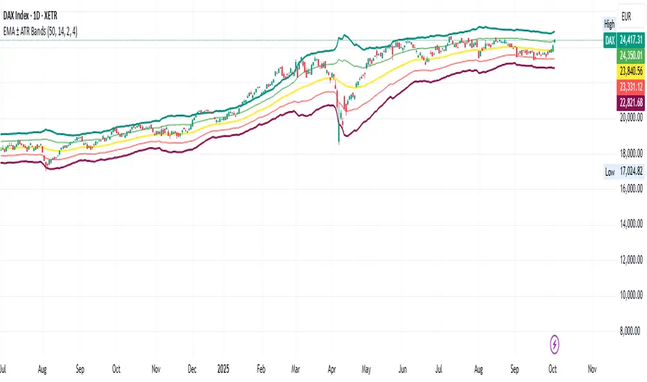
EMA ± ATR BandsPlot the bands from EMA as potential points where may want to enter/exit on principle that price returns to mean over time.
This script was created using Chat GPT.
Quarterly Theory Cycles + Alerts (Weekly/Daily/90-Minute Cycles)Quarterly Theory Cycles (90m • Daily • Weekly)
Purpose
Built for Quarterly Theory. This indicator maps repeating quarters across three rhythms—90-minute, Daily, and Weekly (18:00 NY → 18:00 NY)—so you can track where price is within the current quarter and how it reacts to the previous quarter’s high/low.
Quarter Structure
90-Minute Quarters
Labels:Q1 / Q2 / Q3 / Q4
Sessions: Asia, London, NY, PM (each split into four 90-minute quarters).
Daily Quarters
Labels: [D-Q1 / D-Q2 / D-Q3 / D-Q4
Windows (America/New_York):
D-Q1: 18:00–00:00
D-Q2: 00:00–06:00
D-Q3: 06:00–12:00
D-Q4: 12:00–18:00
Weekly Quarters
Labels: W-Q1 / W-Q2 / W-Q3 / W-Q4
Trading days defined 18:00 NY → 18:00 NY (DST-aware).
W-Q1 = Monday, W-Q2 = Tuesday, W-Q3 = Wednesday, W-Q4 = Thursday
Friday intentionally excluded (no W-Q5) to preserve theory behavior.
Use for higher-timeframe context and weekly narrative (e.g., expansion vs. distribution days).
What It Draws
Live, extending range boxes for the active quarter (H/L updates in real time).
Stored previous quarter’s high/low for each rhythm (90m, Daily, Weekly).
Alerts (Quarterly Theory-friendly )
Fires when price first breaks the previous quarter’s high/low:
90m: “Previous 90min cycle (…) high/low broken”
Daily: “Previous daily cycle (…) high/low broken”
Weekly: “Previous weekly cycle (…) high/low broken”
One alert per side per new quarter—clean signals for liquidity grabs or SSMTs.
Customization
Master Toggles: Show/hide Asia, London, NY, PM, Daily, Weekly blocks fast.
Independent Transparencies: Separate opacity sliders for 90m vs Daily vs Weekly.
Per-Quarter Controls: Toggle range, edit label (defaults already set to Q1 / D-Q1 / W-Q1 formats), and color.
Styling: Optional outlines and labels for minimal or annotated charts.
Time Zones: Use exchange time or a custom UTC offset for session windows. Weekly boundaries always use America/New_York at 18:00.
Notes
Designed for theory workflows: prior-quarter liquidity, session rotation, and narrative alignment, SSMTS.
Friday is excluded from Weekly quarters by design.
Indicator draws ranges and triggers alerts; it does not place trades.

Open Range Breakout (ORB) with Alerts and LabelsThis is a classic 5min ORB indicator that highlights the orb range for your chosen session. This makes it easy to reference the range later in the trading day. In addition to the original orb signals for both buy and sell you can play off that zone for powerful entries later in the session. The signals give TP1 1:1 TP2 2:1
Options
You can set the name of the session
The color of the range.
The buffer for the SL
How many entries for the orb

EQ + Bandas Pro 📊 EQ + Bands Pro is an advanced indicator built on OHLC analysis. It calculates a synthetic equilibrium price and plots dynamic, robust bands that adapt to volatility while filtering outliers. The tool highlights zones of overvaluation and undervaluation, helping traders identify key imbalances, potential reversals, and trend confirmations.

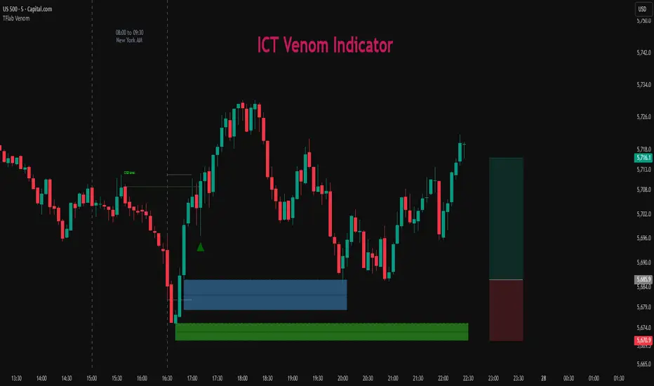
ICT Venom Trading Model [TradingFinder] SMC NY Session 2025SetupIntroduction
The ICT Venom Model is one of the most advanced strategies in the ICT framework, designed for intraday trading on major US indices such as US100, US30, and US500. This model is rooted in liquidity theory, time and price dynamics, and institutional order flow.
The Venom Model focuses on detecting Liquidity Sweeps, identifying Fair Value Gaps (FVG), and analyzing Market Structure Shifts (MSS). By combining these ICT core concepts, traders can filter false breakouts, capture sharp reversals, and align their entries with the real institutional liquidity flow during the New York Session.
Key Highlights of ICT Venom Model :
Intraday focus : Optimized for US indices (US100, US30, US500).
Time element : Critical window is 08:00–09:30 AM (Venom Box).
Liquidity sweep logic : Price grabs liquidity at 09:30 AM open.
Confirmation tools : MSS, CISD, FVG, and Order Blocks.
Dual setups : Works in both Bullish Venom and Bearish Venom conditions.
At its core, the ICT Venom Strategy is a framework that explains how institutional players manipulate liquidity pools by engineering false breakouts around the initial range of the market. Between 08:00 and 09:30 AM New York time, a range called the “Venom Box” is formed.
This range acts as a trap for retail traders, and once the 09:30 AM market open occurs, price usually sweeps either the high or the low of this box to collect stop-loss liquidity. After this liquidity grab, the market often reverses sharply, giving birth to a classic Bullish Venom Setup or Bearish Venom Setup
The Venom Model (ICT Venom Trading Strategy) is not just a pattern recognition tool but a precise institutional trading model based on time, liquidity, and market structure. By understanding the Initial Balance Range, watching for Liquidity Sweeps, and entering trades from FVG zones or Order Blocks, traders can anticipate market reversals with high accuracy. This strategy is widely respected among ICT followers because it offers both risk management discipline and clear entry/exit conditions. In short, the Venom Model transforms liquidity manipulation into actionable trading opportunities.
Bullish Setup :
Bearish Setup :
🔵 How to Use
The ICT Venom Model is applied by observing price behavior during the early hours of the New York session. The first step is to define the Initial Range, also called the Venom Box, which is formed between 08:00 and 09:30 AM EST. This range marks the high and low points where institutional traders often create traps for retail participants. Once the official market opens at 09:30 AM, price usually sweeps either the top or bottom of this box to collect liquidity.
After this liquidity grab, the market tends to reverse in alignment with the true directional bias. To confirm the setup, traders look for signals such as a Market Structure Shift (MSS), Change in State of Delivery (CISD), or the appearance of a Fair Value Gap (FVG). These elements validate the reversal and provide precise levels for trade execution.
🟣 Bullish Setup
In a Bullish Venom Setup, the market first sweeps the low of the Venom Box after 09:30 AM, triggering sell-side liquidity collection. This downward move is often sharp and deceptive, designed to stop out retail long positions and attract new sellers. Once liquidity is taken, the market typically shifts direction, forming an MSS or CISD that signals a reversal to the upside.
Traders then wait for price to retrace into a Fair Value Gap or a demand-side Order Block created during the reversal leg. This retracement offers the ideal entry point for long positions. Stop-loss placement should be just below the liquidity sweep low, while profit targets are set at the Venom Box high and, if momentum continues, at higher session or daily highs.
🟣 Bearish Setup
In a Bearish Venom Setup, the process is similar but reversed. After the Initial Range is defined, if price breaks above the Venom Box high following the 09:30 AM open, it signals a false breakout designed to collect buy-side liquidity. This move usually traps eager buyers and clears out stop-losses above the high.
After the liquidity sweep, confirmation comes through an MSS or CISD pointing to a reversal downward. At this stage, traders anticipate a retracement into a Fair Value Gap or a supply-side Order Block formed during the reversal. Short entries are taken within this zone, with stop-loss positioned just above the liquidity sweep high. The logical profit targets include the Venom Box low and, in stronger bearish momentum, deeper session or daily lows.
🔵 Settings
Refine Order Block : Enables finer adjustments to Order Block levels for more accurate price responses.
Mitigation Level OB : Allows users to set specific reaction points within an Order Block, including: Proximal: Closest level to the current price. 50% OB: Midpoint of the Order Block. Distal: Farthest level from the current price.
FVG Filter : The Judas Swing indicator includes a filter for Fair Value Gap (FVG), allowing different filtering based on FVG width: FVG Filter Type: Can be set to "Very Aggressive," "Aggressive," "Defensive," or "Very Defensive." Higher defensiveness narrows the FVG width, focusing on narrower gaps.
Mitigation Level FVG : Like the Order Block, you can set price reaction levels for FVG with options such as Proximal, 50% OB, and Distal.
CISD : The Bar Back Check option enables traders to specify the number of past candles checked for identifying the CISD Level, enhancing CISD Level accuracy on the chart.
🔵 Conclusion
The ICT Venom Model is more than just a reversal setup; it is a complete intraday trading framework that blends liquidity theory, time precision, and market structure analysis. By focusing on the Initial Range between 08:00 and 09:30 AM New York time and observing how price reacts at the 09:30 AM open, traders can identify liquidity sweeps that reveal institutional intentions.
Whether in a Bullish Venom Setup or a Bearish Venom Setup, the model allows for precise entries through Fair Value Gaps (FVGs) and Order Blocks, while maintaining clear risk management with well-defined stop-loss and target levels.
Ultimately, the ICT Venom Model provides traders with a structured way to filter false moves and align their trades with institutional order flow. Its strength lies in transforming liquidity manipulation into actionable opportunities, giving intraday traders an edge in timing, accuracy, and consistency. For those who master its logic, the Venom Model becomes not only a strategy for entry and exit, but also a deeper framework for understanding how liquidity truly drives price in the New York session.
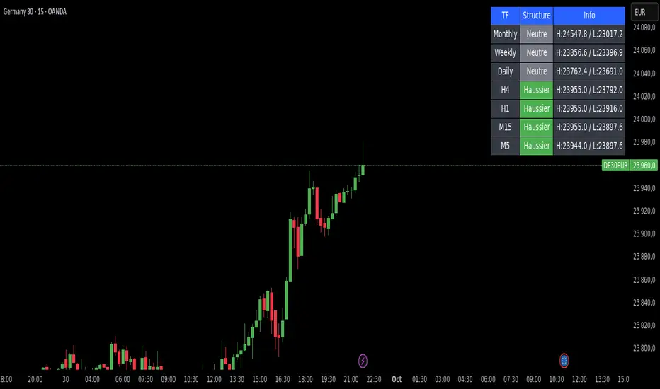
Market Structure DashboardThis indicator displays a **multi-timeframe dashboard** that helps traders track market structure across several horizons: Monthly, Weekly, Daily, H4, H1, M15, and M5.
It identifies the current trend (Bullish, Bearish, or Neutral) based on the progression of **swing highs and lows** (HH/HL, LH/LL).
For each timeframe, the dashboard shows:
* The **current structure** (Bullish, Bearish, Neutral) with a clear color code (green, red, gray).
* **Pivot information**:
* either the latest swing high/low values,
* or the exact date and time of their occurrence (user-selectable in the settings).
An integrated **alert system** notifies you whenever the market structure changes (e.g., "Daily: Neutral → Bullish").
### Key Features:
* Clear overview of multi-timeframe market structures.
* Customizable pivot info display (values or timestamps).
* Built-in alerts on trend changes.
* Compact and readable dashboard, displayed in the top-right corner of the chart.
This tool is ideal for traders who want to quickly assess the **overall market structure** across multiple timeframes and be instantly alerted to potential reversals.
EMA 50/200/100 [NevoxCore]⯁ OVERVIEW
EMA 50/200/100 is a clean EMA trio for trend mapping.
It highlights the classic 50/200 bias, keeps a constant EMA-100 anchor in white, plots cross dots, and can mark the first pullback back to a target EMA within an ATR tolerance.
Solid bias bar coloring (Nevox pink/orange or classic green/red) and compact visuals make it fast and reliable with no repainting.
⯁ HOW IT WORKS
Calculates Fast EMA 50, Slow EMA 200, and an always-on EMA 100 (white).
Bias = Fast vs. Slow: Fast > Slow → long regime; Fast < Slow → short regime.
Cross dots appear at confirmed 50/200 crosses (once per bar close).
First Pullback: after a cross, the script arms a window and marks the first return to the chosen EMA (100 or Fast) within ATR × tolerance.
Bar coloring is solid by regime (pink/orange by default, classic green/red when enabled).
No lookahead; signals confirm on bar close.
⯁ KEY FEATURES
• EMA 50/200 with EMA-100 anchor (always visible, white)
• Cross Up/Down dots (style-configurable)
• First Pullback marker (toggle) with ATR tolerance & window
• Solid bias bar coloring (Nevox or classic)
• Optional bias fill between Fast/Slow
• Minimal 1-cell HUD (OFF by default)
• Ready-made alerts with clean prefixes
⯁ SETTINGS (quick)
Visual: Classic colors toggle; Bias Fill (ON); Fill Transparency (85); Bar Color (solid, ON; auto-disabled when Classic is ON).
Core: Source = Close; EMA Fast = 50; EMA Slow = 200.
Pullback: Show marker (ON); Target EMA = EMA 100; Tolerance × ATR = 0.5; Max Bars After Cross = 40; ATR Length = 14.
HUD: Mini HUD OFF; Position selector.
Status Line: OFF by default (optional EMA values).
⯁ ALERTS (built-in)
• Cross Up (Fast above Slow) — confirmed at bar close
• Cross Down (Fast below Slow) — confirmed at bar close
• First Pullback LONG — first return to target after long cross
• First Pullback SHORT — first return to target after short cross
Prefix: EMA and message includes {{ticker}} {{interval}} @ {{close}}.
Suggested: set TradingView alerts to Once Per Bar Close.
⯁ HOW TO USE
• Read trend quickly: 50 above 200 with a rising 100 = healthy long bias.
• Use the First Pullback to time entries after a cross (default target = EMA 100).
• Tune Tolerance × ATR by symbol/TF; 0.3–0.7 is a good start.
• Keep charts clean: bias fill + barcolor ON; switch to Classic for green/red if preferred.
⯁ WHY IT’S DIFFERENT
It preserves the classic 50/200 logic but adds a consistent EMA-100 anchor, a single, one-shot pullback detector, and clean bias bars — all in a lightweight overlay with no repaint tricks.
⯁ DISCLAIMER
Backtest and paper-trade before using live. Not financial advice. Performance depends on market, timeframe, and parameters.

Adaptive Machine Learning Trading System [PhenLabs]📊Adaptive ML Trading System
Version: PineScript™v6
📌Description
The Adaptive ML Trading System is a sophisticated machine learning indicator that combines ensemble modeling with advanced technical analysis. This system uses XGBoost, Random Forest, and Neural Network algorithms to generate high-confidence trading signals while incorporating robust risk management features. Traders benefit from objective, data-driven decision-making that adapts to changing market conditions.
🚀Points of Innovation
• Machine Learning Ensemble - Three integrated models (XGBoost, Random Forest, Neural Network)
• Confidence-Based Trading - Only executes trades when ML confidence exceeds threshold
• Dynamic Risk Management - ATR-based stop loss and max drawdown protection
• Adaptive Position Sizing - Volatility-adjusted position sizing with confidence weighting
• Real-Time Performance Metrics - Live tracking of win rate, Sharpe ratio, and performance
• Multi-Timeframe Feature Analysis - Adaptive lookback periods for different market regimes
🔧Core Components
• ML Ensemble Engine - Weighted combination of XGBoost, Random Forest, and Neural Network outputs
• Feature Normalization System - Advanced preprocessing with custom tanh/sigmoid activation
• Risk Management Module - Dynamic position sizing and drawdown protection
• Performance Dashboard - Real-time metrics and risk status monitoring
• Alert System - Comprehensive alert conditions for entries, exits, and risk events
🔥Key Features
• High-confidence ML signals with customizable confidence thresholds
• Multiple trading modes (Conservative, Balanced, Aggressive) for different risk profiles
• Integrated stop loss and risk management with ATR-based calculations
• Real-time performance metrics including win rate and Sharpe ratio
• Comprehensive alert system with entry, exit, and risk management notifications
• Visual confidence bands and threshold indicators for easy signal interpretation
🎨Visualization
• ML Signal Line - Primary signal output ranging from -1 to +1
• Confidence Bands - Visual representation of model confidence levels
• Threshold Lines - Customizable buy/sell threshold levels
• Position Histogram - Current market position visualization
• Performance Tables - Real-time metrics display in customizable positions
📖Usage Guidelines
Model Configuration
• Confidence Threshold: Default 0.55, Range 0.5-0.95 - Minimum confidence for signals
• Model Sensitivity: Default 0.9, Range 0.1-2.0 - Adjusts signal sensitivity
• Ensemble Mode: Conservative/Balanced/Aggressive - Trading style preference
• Signal Threshold: Default 0.55, Range 0.3-0.9 - ML signal threshold for entries
Risk Management
• Position Size %: Default 10%, Range 1-50% - Portfolio percentage per trade
• Max Drawdown %: Default 15%, Range 5-30% - Maximum allowed drawdown
• Stop Loss ATR: Default 2.0, Range 0.5-5.0 - Stop loss in ATR multiples
• Dynamic Sizing: Default true - Volatility-based position adjustment
Display Settings
• Show Signals: Default true - Display entry/exit signals
• Show Threshold Signals: Default true - Display ±0.6 threshold crosses
• Show Confidence Bands: Default true - Display ML confidence levels
• Performance Dashboard: Default true - Show metrics table
✅Best Use Cases
• Swing trading with 1-5 day holding periods
• Trend-following strategies in established trends
• Volatility breakout trading during high-confidence periods
• Risk-adjusted position sizing for portfolio management
• Multi-timeframe confirmation for existing strategies
⚠️Limitations
• Requires sufficient historical data for accurate ML predictions
• May experience low confidence periods in choppy markets
• Performance varies across different asset classes and timeframes
• Not suitable for very short-term scalping strategies
• Requires understanding of basic risk management principles
💡What Makes This Unique
• True machine learning ensemble with multiple model types
• Confidence-based trading rather than simple signal generation
• Integrated risk management with dynamic position sizing
• Real-time performance tracking and metrics
• Adaptive parameters that adjust to market conditions
🔬How It Works
Feature Calculation: Computes 20+ technical features from price/volume data
Feature Normalization: Applies custom normalization for ML compatibility
Ensemble Prediction: Combines XGBoost, Random Forest, and Neural Network outputs
Signal Generation: Produces confidence-weighted trading signals
Risk Management: Applies position sizing and stop loss rules
Execution: Generates alerts and visual signals based on thresholds
💡Note:
This indicator works best on daily and 4-hour timeframes for most assets. Ensure you understand the risk management settings before live trading. The system includes automatic risk-off modes that halt trading during excessive drawdown periods.