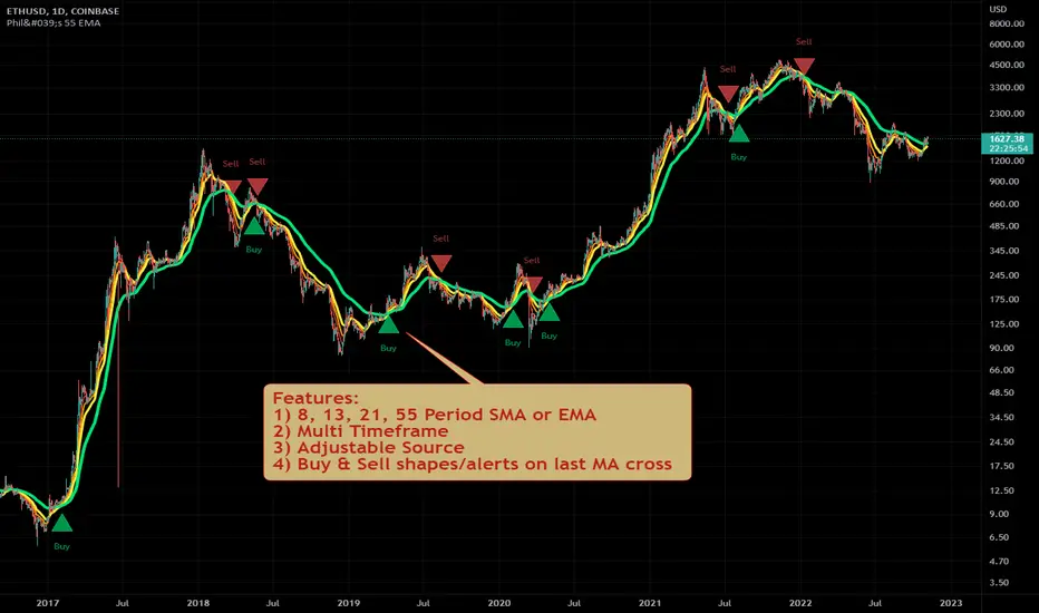
Philakone 55 EMA Swing Trading StrategyThis strategy was inspired by Philkone Crypto's "Lesson 12: Let's Learn Advanced 55 EMA Strategy" video.
steemit.com
Supports Buy and Sell Condition alerts and displays arrows on the chart.
Search in scripts for "跨境通12月4日地天板"
Ichimoku Kinko Hyo + HULL-MA_X + MacDThe Ichimoku Kinko Hyo system includes five kinds of signal, of which this strategy uses the most recent of ones i.e. Tenkan Sen / Kijun Sen Cross and price crosses the Kijun Sen. As the Chikou Span, Senkou Span A and Senkou Span B are shifted into the past/future, the trigger signals will be only be used for visual confirmation and not part of the strategy.
The Tenkan Sen, also known as the Turning or Conversion line, is a moving average of the highest high and lowest low over the last 9 periods in this strategy.
The Kijun Sen, also known as the Standard or Base line, is a moving average of the highest high and lowest low over the last 24 periods in this strategy.
The Chikou Span, also known as the Lagging line, is the closing price plotted 24 periods behind in this strategy.
The Senkou Span A, also known as the 1st leading line, is a moving average of the Tenkan Sen and Kijun Sen and is plotted 24 periods ahead in this strategy.
The Senkou Span B, also known as the 2nd leading line, is a moving average of the highest high and lowest low over the last 51 trading days is plotted 24 periods ahead in this strategy.
Moving average convergence divergence (MaCD) is a trend-following momentum indicator that shows the relationship between two moving averages of prices. The MaCD is calculated in this strategy by subtracting the 24-day exponential moving average (EMA) from the 12-day EMA. A nine-day EMA of the MACD, called the "signal line", aMaCD in this case, is then plotted on top of the MaCD. In this strategy, MaCD/ aMaCD Cross is functioning as a trigger for buy and sell signals.
As with most technical analysis methods, Ichimoku is likely to produce frequent conflicting signals in non-trending markets, So in addition to Ichimoku Kinko Hyo, the Hull MA is popular amongst some day traders, as the indicator which in combination with MaCD attempts to give an accurate signal by eliminating lags and improving the smoothness of the line.
Alan Hull, developed this moving average indicator and hence it’s called the Hull MA.
Now, let’s dissect how the Hull moving average is calculated.
The Hull MA involves the weighted moving average (WMA) in its calculation.
First, calculate the WMA with period (n / 2) and multiply this by 2. Remember ‘n’ is the time period configurable based on the trader’s requirement. The default setting is 12 periods in this strategy, fast Hull MA crossing slow Hull MA will generate a circle on charts.
Second, calculate the WMA for period “n” and subtract if from the first step. Thirdly, calculate the weighted moving average with period sqrt (n) using the data from the second step. You can take a look at the below formula:
Hull MA= WMA (2*WMA (n/2) − WMA (n)), sqrt (n))
The Hull MA Cross in combination with Tenkan Sen / Kijun Sen Cross and MaCD tries to give an accurate signal by eliminating lags and improve the smoothness of price activity. Please note that price trends can and do change often, so your readings of the charts and this trading system should be probabilistic, rather than predictive.

Pullback Trading Tool R5-65 by JustUncleLBy request this is an updated version of the "PullBack Trading Tool": removes experimental "OCC" channel, added option to display ribbons or just single moving average lines, added alert arrows for "PB" exits, added alertcondition for TV alarm subsystem, added some extract options for Pivot points and general cleanup of code.
Description:
This project incorporates the majority of the indicators needed to analyse and trade Trends for Pullbacks, swings and reversals.
Incorporated within this tool are the following indicators:
1. Major industry (Banks) recognised important EMAs in an EMA Ribbon:
Lime = EMA5 (Optional Display)
DodgerBlue = EMA12 (Optional Display)
Red = EMA36 (Optional display)
Green = EMA89
Blue = EMA200
Black = EMA633
2. The 5 EMA (default) High/Low/Close Price Action Channel (PAC), the PAC channel display is disabled by default.
3. Optionally display Fractals and optional Fractal levels
4. Optional HH, LH, LL, HL finder.
5. Optional Buy/Sell "PB" exit Alerts with Optional 200EMA filter.
6. Coloured coded Bar high lighting based on the PAC:
blue = bar closed above PAC
red = bar closed below PAC
gray = bar closed inside PAC
7. Alert condition sent to TradingView's Alarm subsystem for PB exits.
8. Pivot points with optional labels.
9. EMA5-12 Ribbon is displayed by default.
10.EMA12-36 Ribbon is displayed by default
Set up and hints:
I am unable to provide a full description here, as Pullback Trading incorporates a full trading Methodology, there are a number of articles and books written on the subject.
Set the chart to Heikin Ashi Candles (optional).
I also add a "Sweetspot Gold R3" indicator to the chart as well to help with support and resistance finding and shows where the important "00" lines are.
First on a weekly basis say Sunday night or Monday morning, analyse the Daily and Weekly charts to establish overall trends, and support/resistant levels. Draw significant mini trend lines (2/3 TL), vertical trend lines (VTL) and S/R levels. Can use the Pivots points to guide VTL drawing and Fractals to help guide 2/3 TL drawing.
Once the trend direction and any potential major reversals highlighted, drop down to lower timeframe chart and draw appropriate mini Trend line (2/3 TL) matching the established momentum direction. Take note of potential pull backs from and of the EMAs, in particular the EMA5-12 ribbon, EMA12-36 Ribbon and the 200EMA. Can use the Pivots and/or Fractals points to guide your 2/3 TL drawing.
Set a TradingView alarm on the "PBTOOL alert", with the default settings this normally occurs before or during the Break of the manually drawn TL lines.
Once alerted check to see if the TL is broken and is returning to trend away from the EMA lines, this is indicated by bar colour change to trend directional colour.
You can trade that alert or drop down to even lower time frames and perform the same TL analysis there to find trades at the lower TF. Trading at lower TF you will allow tighter Stop loss settings.
Other than the "SweetSpot Gold R3" indicator, you should not need any other indicator to successfully trade trends for Pullbacks and reversals. If you really want another indicator I suggest a momentum one for example: AO ( Awesome Oscillator ), MACD or Squeeze Momentum.

Spartan Trader FX IndicatorUnofficial (I am not affiliated to www.spartantraderfx.com in any way) combo indicator providing all the indicators needed for their trading system (default coloring as presented in the materials):
EMA 12 line
EMA 36 line
EMA 200 line
EMA 633 line
EMA 200 and EMA 633 volatility zone
EMA 12/36 crossover arrows
heiken ashi color overlay(helpful when trying to see true open and close of candles using regular candlesticks)

Scalping Swing Trading Tool R1-4 by JustUncleLDescription:
This study project is a "Scalping Swing trading Tool" and is an alternative to the "Scalping Pullback Tool R1". It is designed for a two pane TradingView chart layout :
the first pane set to 15min Time Frame;
the second pane set to 1min Time Frame(TF).
The tools incorporates the majority of the indicators needed to analyse and scalp Trends for Swings, PullBacks and reversals on 15min charts and 1min charts.
Incorporated within this tool are the following indicators:
1. The following EMAs are drawn automatically:
Green = EMA89 (15min TF) = EMA75 (1min TF)
Blue = EMA200 (15min TF) = EMA180 (1min TF)
Black = EMA633 (15min TF) = EMA540 (1min TF)
2. The 10EMA (default) High/Low+Close Price Action Channel (PAC), the PAC channel
display is disabled by default.
3. Optionally display Fractals and optional Fractal levels
4. Optional HH, LH, LL, HL finder.
5. Coloured coded Bar high lighting based on the PAC:
blue = bar closed above PAC
red = bar closed below PAC
gray = bar closed inside PAC
lime Line = EMA10 of bar close
6. Pivot points (disables Fractals automatically when selected) with optional labels.
7. EMA5-12 Channel is displayed by default.
8. EMA12-36 Ribbon is displayed by default
9. Optionally display EMA36 and PAC instead of EMA12-36 Ribbon.
Set up and hints:
I am unable to provide a full description here, as Pullback Trading incorporates a full trading Methodology, there are a number of articles and books written on the subject.
Set to two pane TradingView chart, set first pane to 15Min and second to 1min.
Set the chart to Heikin Ashi Candles (optional).
I also add a "Sweetspot Gold2" indicator to the chart as well to help with support and resistance finding and shows where the important "00" lines are.
Use the EMA200 on the 15min pane as the anchor. So when prices above EMA200 we only trade long (buy) and when prices below the EMA200 we only trade short (sell).
On the 15min chart draw any obvious Vertical Trend Lines (VTL), use Pivots point as a guide.
On the 15min chart what we’re looking for price to Pullback into the EMA5-12 Channel or EMA12-36 ribbon, we draw Trendlines uitilising the Pivot points or Fractals to guide your TL drawing.
On the 15min chart look for the trend to resume and break through the drawn TL. The bar color needs to change back to the trend direction colour to confirm as a break.
Now this break can be traded as a 15min trade or now look to the 1min chart.
On the 1min chart draw any Pullback into any of the EMAs.
On the 1min chart look for the trend to resume and break through the drawn TL. The bar color needs to change back to the trend direction colour to confirm as a break.
Now this break can be traded as a 1min trade.
There is also an option to select Pristine (ie Ideal) filtered Fractals, which look like tents or V shape 5-candle patterns. These are actually used to calculate the Pivot points as well.
Other than the "SweetSpot Gold2" indicator, you should not need any other indicator to successfully trade trends for Pullbacks and reversals. If you really want another indicator use the AO (Awesome Oscillator) as it is momentum based.

Murray Math LevelsThe original script was posted on ProRealCode by user supertiti.
The Murray Math lines levels are determined within some principles of Gann levels and candlesticks formations. The Murray Math levels act pretty much like pivot and support/resistance areas.
1. Line 8/8 - 0/8 (Ultimate Support and Ultimate Resistance).
Those lines are the most strong concerning Support and resistance.
2. Line 7/8 (Weak, Place to Stop and Reverse).
This line is weak. If suddenly the price was going too fast and too far and stops around this line it means the price will reverse down very soon. If the price did not stop near this line this price will continue the movement to the line 8/8.
3. Line 1/8 (Weak, Place to Stop and Reverse).
This line is weak. If suddenly the price was going too fast and too far and stops around this line it means the price will reverse up very soon. If the price did not stop near this line this price will continue the movement down to the line 0/8.
4. Line 2/8 and 6/8 (Pivot, Reverse)
Those two lines yield the line 4/8 only to the strength to reverse the price movement.
5. Line 5/8 (Top of Trading Range)
The price is spending the about 40% of the time on the movement between the lines 5/8 and 3/8. If the price is moving near line 5/8 and stopping near the line during the 10 - 12 days so it means that it is necessary to sell in this "bonus zone" (some people are doing like this) but if the price is keeping the tendency to stay above 5/8 line, so it means that the price will be above. But if the price is droping below 5/8 line it means that the price will continue falling to the next level of resistance.
6. Line 3/8 (Bottom of Trading Range).
If the price is below this line and in uptrend it means that it will be very difficult for the price to break this level. If the price broke this line during the uptrend and staying above during the 10- 12 days it means that the price will be above this line during the 40% of its time moving between this line and 5/8 line.
7. Line 4/8 (Major Support/Resistance Line).
It is the major line concerning support and resistance. This level is the better for the new sell or buy. It is the strong level of support of the price is above 4/8. It is the fine resistance line if the price is below this 4/8 line.
Candlestick Trend Indicator v0.5 by JustUncleLRequested Update to this Indicator alert project. In this update I have added the option to be able select which Price Action candles you want included in the display and the generated alarm Alert. Other changes also included in this update:
Also added a Price Action candle for "Last Fractal S/R Break", this also a good continuation indication.
Added option to select a different moving average types for directional MA line.
Modified some default settings, using HullMA instead of Zero Lag EMA and standard MACD settings(12,26,9).
Description:
This is a trend following indicator and alert for Binary Options based on Candlestick patterns and trend line -
NOTE: original system was a forex trading system.
This code combines a number of indicators to create an overall trading strategy.
The indicator recognises and displays some useful candle named defined patterns that are used to support trend continuation:
Bearish + Bullish PinBars
Dark Cloud Cover
Piecing Line
Bullish + Bearish Harami
Bullish + Bearish Engulfing Candle
Bullish + Bearish Last Fractal S/R break
Also recognises main Price Action candles from ChrisMoody (CM), the four(4) price action patterns are colored coded bars:
Yellow = Inside Bar - breakout/continuance
Orange = Outside Bar - breakout/continuance
Aqua/Fuschia = Up/Down Shaved Bars - Buying/Selling pressure
Red/Green = Possible reversal PinBars - Reverse Down / reverse Up
The highlighted candles (maroon and darker green) represent the defined PA patterns that have been confirmed following the current trend direction that is indicated by the Hull MA(20) line (can select a different type of MA, or even disable) and confirmed by MACD direction (can be disabled). The confirmed Alerts are indication by green (buy) and red (sell) dots at the bottom of the chart. An alert is generated from this selection for the alert condition of the alarming system.
The fractal upper/lower break lines are also draw, if the (optional) last fractal break line is broken by a highlighted bar then this indicates a stronger trend conformation.
The MACD indicator MACD DEUTER 2 colour(12,26,9) you can visually see the MACD histogram colours with MACD direction - needs "MACD DEUTER 2 colour" indicator.
This multi-indicator set up is suitable for 1hr, 4hr and daily charts with 1-4 candle expiry.
References and Inspiration from:
Fractal Levels by RicardoSantos
Almost Zero Lag EMA
Candlestick Patterns With EMA by rmwaddelljr
CM_Price-Action-Bars by ChrisMoody
www.forexstrategiesresources.com
"Scalp Jockey - MTF MA Cross Visual Strategizer by JayRogers"

Sladkaya Bulochka PosledovatelnostiSerial number of the same color candles - a popular method of how to find the exact entry zones and determine the trends and kickbacks.
The number of consecutive candles usually starts from 3 and up to 12 in some strategies.
5 candles in sequence - one of the most popular signals. Login at the close of the 5th candle.
---------------------------------------------
Последовательное число свечей одинакового цвета - популярный метод как поиска точных зон входа, так и определения трендов и откатов.
Число последовательных свечей, как правило, начинается с 3 и доходит до 12 в некоторых стратегиях.
5 свечей в последовательности - один из наиболее популярных сигналов. Вход на закрытии 5й свечи.
MACD trend heatmap (by ChartArt)This is an overlay indicator which uses the classic period settings and signals from the MACD (Moving Average Convergence/Divergence) indicator to overlay a heatmap using all the information the MACD generates with its three periods (12,26,9).
The first two moving averages which the MACD uses (12 and 26) can be plotted on the chart like usual EMAs.
In addition to the background color function (the heatmap) and the EMAs, there is an optional bar color alert when the uptrend or the downtrend as measured by the MACD appears to be very strong.

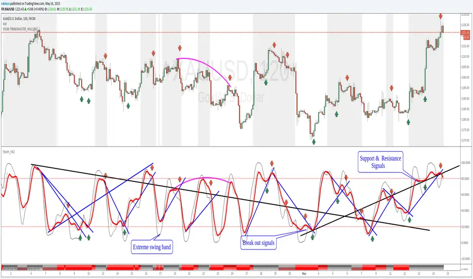
Stoch_VX2Nothing New about a Stochastic but maybe in how you use them ( Other than Over bought / Sold cross over & divergence signals )
Running 3 bands
Standard stoch & tops & bottoms swing band
Optimised variables 12, 5 , 3 or fib 13, 5, 3 / - 12 / 3 / 3 a little bit tighter to combine both smoothness & accuracy. These are my own personal setting inc. Strategy.
MACD Color Trawler (by ChartArt)This version of the MACD indicator is 'trawling' (checking) if the MACD histogram and the zero line crossing with the MACD line are both positive or negative. The idea behind this is to show areas with higher or lower risk.
Features:
1. Enable the bar color
2. Enable the background color
3. Change zero line value
FYI:
"The MACD-Histogram is an indicator of an indicator. In fact, MACD is also an indicator of an indicator. This means that the MACD-Histogram is the fourth derivative of price."
First derivative: 12-day EMA and 26-day EMA
Second derivative: MACD (12-day EMA less the 26-day EMA)
Third derivative: MACD signal line (9-day EMA of MACD)
Fourth derivative: MACD-Histogram (MACD less MACD signal line)
Source: stockcharts.com

Multi Momentum 10/21/42/63 — Histogram + 2xSMAMY MM INDICATOR INDIRED BY KARADI
It averages four rate-of-change snapshots of price, all anchored at today’s close.
If “Show as %” is on, the value is multiplied by 100.
Each term is a simple momentum/ROC over a different lookback.
Combining 10, 21, 42, 63 bars blends short, medium, and intermediate horizons into one number.
Positive MM → average upward pressure across those horizons; negative MM → average downward pressure.
Why those lengths?
They roughly stack into ~2× progression (10→21≈2×10, 21→42=2×21, 63≈1.5×42). That creates a “multi-scale” momentum that’s less noisy than a single fast ROC but more responsive than a long ROC alone.
How to read the panel
Gray histogram = raw Multi-Momentum value each bar.
SMA Fast/Slow lines (defaults 12 & 26 over the MM values) = smoothing of the histogram to show the trend of momentum itself.
Typical signals
Zero-line context:
Above 0 → bullish momentum regime on average.
Below 0 → bearish regime.
Crosses of SMA Fast & Slow: momentum trend shifts (fast above slow = improving momentum; fast below slow = deteriorating).
Histogram vs SMA lines: widening distance suggests strengthening momentum; narrowing suggests momentum is fading.
Divergences: price makes a new high/low but MM doesn’t → potential exhaustion.
Compared to a classic ROC
A single ROC(20) is very sensitive to that one window.
MM averages several windows, smoothing idiosyncrasies (e.g., a one-off spike 21 bars ago) and reducing “lookback luck.”
Settings & customization
Lookbacks (10/21/42/63): you can tweak for your asset/timeframe; the idea is to mix short→medium horizons.
Percent vs raw ratio: percent is easier to compare across symbols.
SMA lengths: shorter = more reactive but choppier; longer = smoother but slower.
Practical tips
Use regime + signal: trade longs primarily when MM>0 and fast SMA>slow SMA; consider shorts when MM<0 and fast

S&P500 Net Issues Block 12Description:
This indicator calculates and plots net advancers minus decliners for 13 predefined blocks of S&P 500 stocks. Each block represents a sector or a selected subset of stocks.
Features:
Shows net issues (advancers – decliners) for each block separately.
13 blocks plotted with distinct colors for easy identification.
Fully compatible with 1-minute, intraday, or higher timeframe charts.
Ideal for identifying sector momentum and market breadth trends.
Can be used standalone or combined with other indicators such as market indices (e.g., S&P 500 futures or TICK).
Usage:
Green/red/blue/orange lines represent different blocks; positive values indicate more advancing stocks than declining, negative values indicate more declining stocks.
Best viewed on intraday charts for short-term market breadth analysis.
Disclaimer:
This indicator is for educational and analytical purposes only. Not a buy/sell signal. Use proper risk management and verify data before trading.

EvoTrend-X Indicator — Evolutionary Trend Learner ExperimentalEvoTrend-X Indicator — Evolutionary Trend Learner
NOTE: This is an experimental Pine Script v6 port of a Python prototype. Pine wasn’t the original research language, so there may be small quirks—your feedback and bug reports are very welcome. The model is non-repainting, MTF-safe (lookahead_off + gaps_on), and features an adaptive (fitness-based) candidate selector, confidence gating, and a volatility filter.
⸻
What it is
EvoTrend-X is adaptive trend indicator that learns which moving-average length best fits the current market. It maintains a small “population” of fast EMA candidates, rewards those that align with price momentum, and continuously selects the best performer. Signals are gated by a multi-factor Confidence score (fitness, strength vs. ATR, MTF agreement) and a volatility filter (ATR%). You get a clean Fast/Slow pair (for the currently best candidate), optional HTF filter, a fitness ribbon for transparency, and a themed info panel with a one-glance STATUS readout.
Core outputs
• Selected Fast/Slow EMAs (auto-chosen from candidates via fitness learning)
• Spread cross (Fast – Slow) → visual BUY/SELL markers + alert hooks
• Confidence % (0–100): Fitness ⊕ Distance vs. ATR ⊕ MTF agreement
• Gates: Trend regime (Kaufman ER), Volatility (ATR%), MTF filter (optional)
• Candidate Fitness Ribbon: shows which lengths the learner currently prefers
• Export plot: hidden series “EvoTrend-X Export (spread)” for downstream use
⸻
Why it’s different
• Evolutionary learning (on-chart): Each candidate EMA length gets rewarded if its slope matches price change and penalized otherwise, with a gentle decay so the model forgets stale regimes. The best fitness wins the right to define the displayed Fast/Slow pair.
• Confidence gate: Signals don’t light up unless multiple conditions concur: learned fitness, spread strength vs. volatility, and (optionally) higher-timeframe trend.
• Volatility awareness: ATR% filter blocks low-energy environments that cause death-by-a-thousand-whipsaws. Your “why no signal?” answer is always visible in the STATUS.
• Preset discipline, Custom freedom: Presets set reasonable baselines for FX, equities, and crypto; Custom exposes all knobs and honors your inputs one-to-one.
• Non-repainting rigor: All MTF calls use lookahead_off + gaps_on. Decisions use confirmed bars. No forward refs. No conditional ta.* pitfalls.
⸻
Presets (and what they do)
• FX 1H (Conservative): Medium candidates, slightly higher MinConf, modest ATR% floor. Good for macro sessions and cleaner swings.
• FX 15m (Active): Shorter candidates, looser MinConf, higher ATR% floor. Designed for intraday velocity and decisive sessions.
• Equities 1D: Longer candidates, gentler volatility floor. Suits index/large-cap trend waves.
• Crypto 1H: Mid-short candidates, higher ATR% floor for 24/7 chop, stronger MinConf to avoid noise.
• Custom: Your inputs are used directly (no override). Ideal for systematic tuning or bespoke assets.
⸻
How the learning works (at a glance)
1. Candidates: A small set of fast EMA lengths (e.g., 8/12/16/20/26/34). Slow = Fast × multiplier (default ×2.0).
2. Reward/decay: If price change and the candidate’s Fast slope agree (both up or both down), its fitness increases; otherwise decreases. A decay constant slowly forgets the distant past.
3. Selection: The candidate with highest fitness defines the displayed Fast/Slow pair.
4. Signal engine: Crosses of the spread (Fast − Slow) across zero mark potential regime shifts. A Confidence score and gates decide whether to surface them.
⸻
Controls & what they mean
Learning / Regime
• Slow length = Fast ×: scales the Slow EMA relative to each Fast candidate. Larger multiplier = smoother regime detection, fewer whipsaws.
• ER length / threshold: Kaufman Efficiency Ratio; above threshold = “Trending” background.
• Learning step, Decay: Larger step reacts faster to new behavior; decay sets how quickly the past is forgotten.
Confidence / Volatility gate
• Min Confidence (%): Minimum score to show signals (and fire alerts). Raising it filters noise; lowering it increases frequency.
• ATR length: The ATR window for both the ATR% filter and strength normalization. Shorter = faster, but choppier.
• Min ATR% (percent): ATR as a percentage of price. If ATR% < Min ATR% → status shows BLOCK: low vola.
MTF Trend Filter
• Use HTF filter / Timeframe / Fast & Slow: HTF Fast>Slow for longs, Fast threshold; exit when spread flips or Confidence decays below your comfort zone.
2) FX index/majors, 15m (active intraday)
• Preset: FX 15m (Active).
• Gate: MinConf 60–70; Min ATR% 0.15–0.30.
• Flow: Focus on session opens (LDN/NY). The ribbon should heat up on shorter candidates before valid crosses appear—good early warning.
3) SPY / Index futures, 1D (positioning)
• Preset: Equities 1D.
• Gate: MinConf 55–65; Min ATR% 0.05–0.12.
• Flow: Use spread crosses as regime flags; add timing from price structure. For adds, wait for ER to remain trending across several bars.
4) BTCUSD, 1H (24/7)
• Preset: Crypto 1H.
• Gate: MinConf 70–80; Min ATR% 0.20–0.35.
• Flow: Crypto chops—volatility filter is your friend. When ribbon and HTF OK agree, favor continuation entries; otherwise stand down.
⸻
Reading the Info Panel (and fixing “no signals”)
The panel is your self-diagnostic:
• HTF OK? False means the higher-timeframe EMAs disagree with your intended side.
• Regime: If “Chop”, ER < threshold. Consider raising the threshold or waiting.
• Confidence: Heat-colored; if below MinConf, the gate blocks signals.
• ATR% vs. Min ATR%: If ATR% < Min ATR%, status shows BLOCK: low vola.
• STATUS (composite):
• BLOCK: low vola → increase Min ATR% down (i.e., allow lower vol) or wait for expansion.
• BLOCK: HTF filter → disable HTF or align with the HTF tide.
• BLOCK: confidence → lower MinConf slightly or wait for stronger alignment.
• OK → you’ll see markers on valid crosses.
⸻
Alerts
Two static alert hooks:
• BUY cross — spread crosses up and all gates (ER, Vol, MTF, Confidence) are open.
• SELL cross — mirror of the above.
Create them once from “Add Alert” → choose the condition by name.
⸻
Exporting to other scripts
In your other Pine indicators/strategies, add an input.source and select EvoTrend-X → “EvoTrend-X Export (spread)”. Common uses:
• Build a rule: only trade when exported spread > 0 (trend filter).
• Combine with your oscillator: oscillator oversold and spread > 0 → buy bias.
⸻
Best practices
• Let it learn: Keep Learning step moderate (0.4–0.6) and Decay close to 1.0 (e.g., 0.99–0.997) for smooth regime memory.
• Respect volatility: Tune Min ATR% by asset and timeframe. FX 1H ≈ 0.10–0.20; crypto 1H ≈ 0.20–0.35; equities 1D ≈ 0.05–0.12.
• MTF discipline: HTF filter removes lots of “almost” trades. If you prefer aggressive entries, turn it off and rely more on Confidence.
• Confidence as throttle:
• 40–60%: exploratory; expect more signals.
• 60–75%: balanced; good daily driver.
• 75–90%: selective; catch the clean stuff.
• 90–100%: only A-setups; patient mode.
• Watch the ribbon: When shorter candidates heat up before a cross, momentum is forming. If long candidates dominate, you’re in a slower trend cycle.
⸻
Non-repainting & safety notes
• All request.security() calls use lookahead=barmerge.lookahead_off, gaps=barmerge.gaps_on.
• No forward references; decisions rely on confirmed bar data.
• EMA lengths are simple ints (no series-length errors).
• Confidence components are computed every bar (no conditional ta.* traps).
⸻
Limitations & tips
• Chop happens: ER helps, but sideways microstructure can still flicker—use Confidence + Vol filter as brakes.
• Presets ≠ oracle: They’re sensible baselines; always tune MinConf and Min ATR% to your venue and session.
• Theme “Auto”: Pine cannot read chart theme; “Auto” defaults to a Dark-friendly palette.
⸻
Publisher’s Screenshots Checklist
1) FX swing — EURUSD 1H
• Preset: FX 1H (Conservative)
• Params: MinConf=70, ATR Len=14, Min ATR%=0.12, MTF ON (TF=4H, 20/50)
• Show: Clear BUY cross, STATUS=OK, green regime background; Fitness Ribbon visible.
2) FX intraday — GBPUSD 15m
• Preset: FX 15m (Active)
• Params: MinConf=60, ATR Len=14, Min ATR%=0.20, MTF ON (TF=60m)
• Show: SELL cross near London session open. HTF lines enabled (translucent).
• Caption: “GBPUSD 15m • Active session sell with MTF alignment.”
3) Indices — SPY 1D
• Preset: Equities 1D
• Params: MinConf=60, ATR Len=14, Min ATR%=0.08, MTF ON (TF=1W, 20/50)
• Show: Longer trend run after BUY cross; regime shading shows persistence.
• Caption: “SPY 1D • Trend run after BUY cross; weekly filter aligned.”
4) Crypto — BINANCE:BTCUSDT 1H
• Preset: Crypto 1H
• Params: MinConf=75, ATR Len=14, Min ATR%=0.25, MTF ON (TF=4H)
• Show: BUY cross + quick follow-through; Ribbon warming (reds/yellows → greens).
• Caption: “BTCUSDT 1H • Momentum break with high confidence and ribbon turning.”

Z-Score Mean Reversion StrategyBased on Indicator "Rolling Z- Score trend" by QuantAlgo
The Z-Score Mean Reversion Strategy is a statistical trading approach that exploits price extremes and their tendency to return to average levels. It uses the Z-Score indicator to identify when an asset has deviated significantly from its statistical mean, creating high-probability reversal opportunities.
Core Concept:
Z-Score measures how many standard deviations price is from its moving average
When Z-Score reaches extreme levels (±1.5 or more), price is statistically "stretched"
The strategy trades the expected "snap back" to the mean
Works best in ranging or mean-reverting markets
How It Works:
LONG Entry: When price becomes oversold (Z-Score < -1.5), expect upward reversion
SHORT Entry: When price becomes overbought (Z-Score > +1.5), expect downward reversion
Exit: When price returns closer to the mean or reaches opposite extreme
Risk Management: Stop loss at -3% and take profit at +5% by default
🎯 Best Settings by Market & Timeframe
Cryptocurrency (High Volatility)
Preset: Scalping
Timeframe: 15m - 1H
Lookback: 10-15 periods
Entry Threshold: 1.0 - 1.5
Stop Loss: 2-3%
Take Profit: 3-5%
Notes: Crypto moves fast; use tighter parameters for quicker signals
Forex (Medium Volatility)
Preset: Default or Swing Trading
Timeframe: 1H - 4H
Lookback: 20-25 periods
Entry Threshold: 1.5 - 2.0
Stop Loss: 1-2%
Take Profit: 2-4%
Notes: Works well on major pairs during normal market conditions
Stocks (Lower Volatility)
Preset: Swing Trading
Timeframe: 4H - Daily
Lookback: 25-30 periods
Entry Threshold: 1.5 - 1.8
Stop Loss: 2-4%
Take Profit: 4-8%
Notes: Best on liquid stocks; avoid during earnings or major news
Indices (Trend + Ranging)
Preset: Trend Following
Timeframe: Daily - Weekly
Lookback: 35-50 periods
Entry Threshold: 2.0 - 2.5
Stop Loss: 3-5%
Take Profit: 5-10%
Notes: Higher threshold reduces false signals; captures major reversals
⚙️ Optimal Configuration Guide
Conservative (Lower Risk, Fewer Trades)
Lookback Period: 30-40
Entry Threshold: 2.0-2.5
Exit Threshold: 0.8-1.0
Stop Loss: 3-4%
Take Profit: 6-10%
Momentum Filter: ON
Balanced (Recommended Starting Point)
Lookback Period: 20-25
Entry Threshold: 1.5-1.8
Exit Threshold: 0.5-0.6
Stop Loss: 2-3%
Take Profit: 4-6%
Momentum Filter: OFF
Aggressive (Higher Risk, More Trades)
Lookback Period: 10-15
Entry Threshold: 1.0-1.2
Exit Threshold: 0.3-0.4
Stop Loss: 1-2%
Take Profit: 2-4%
Momentum Filter: OFF
💡 Pro Tips for Best Results
When the Strategy Works Best:
✅ Ranging markets with clear support/resistance
✅ High liquidity assets (major pairs, large-cap stocks)
✅ Normal market conditions (avoid during crashes or parabolic runs)
✅ Mean-reverting assets (avoid strong trending stocks)
When to Avoid:
❌ Strong trending markets (price won't revert)
❌ Low liquidity / low volume periods
❌ Major news events (earnings, FOMC, NFP)
❌ Market crashes or euphoria phases
Optimization Process:
Start with "Default" preset on your chosen timeframe
Backtest 6-12 months to see performance
Adjust Entry Threshold first (lower = more trades, higher = fewer but stronger signals)
Fine-tune Stop Loss/Take Profit based on average trade duration
Consider Momentum Filter if getting too many false signals
Key Metrics to Monitor:
Win Rate: Target 50-60% (mean reversion typically has moderate win rate)
Profit Factor: Aim for >1.5
Average Trade Duration: Should match your timeframe (scalping: minutes/hours, swing: days)
Max Drawdown: Keep under 20% of capital
📈 Quick Start Recommendation
For most traders, start here:
Timeframe: 1H or 4H
Preset: Default (Lookback 20, Threshold 1.5)
Stop Loss: 3%
Take Profit: 5%
Momentum Filter: OFF (turn ON if too many false entries)
Test on BTCUSD, EURUSD, or SPY first, then adapt to your preferred instruments!

Small Business Economic Conditions - Statistical Analysis ModelThe Small Business Economic Conditions Statistical Analysis Model (SBO-SAM) represents an econometric approach to measuring and analyzing the economic health of small business enterprises through multi-dimensional factor analysis and statistical methodologies. This indicator synthesizes eight fundamental economic components into a composite index that provides real-time assessment of small business operating conditions with statistical rigor. The model employs Z-score standardization, variance-weighted aggregation, higher-order moment analysis, and regime-switching detection to deliver comprehensive insights into small business economic conditions with statistical confidence intervals and multi-language accessibility.
1. Introduction and Theoretical Foundation
The development of quantitative models for assessing small business economic conditions has gained significant importance in contemporary financial analysis, particularly given the critical role small enterprises play in economic development and employment generation. Small businesses, typically defined as enterprises with fewer than 500 employees according to the U.S. Small Business Administration, constitute approximately 99.9% of all businesses in the United States and employ nearly half of the private workforce (U.S. Small Business Administration, 2024).
The theoretical framework underlying the SBO-SAM model draws extensively from established academic research in small business economics and quantitative finance. The foundational understanding of key drivers affecting small business performance builds upon the seminal work of Dunkelberg and Wade (2023) in their analysis of small business economic trends through the National Federation of Independent Business (NFIB) Small Business Economic Trends survey. Their research established the critical importance of optimism, hiring plans, capital expenditure intentions, and credit availability as primary determinants of small business performance.
The model incorporates insights from Federal Reserve Board research, particularly the Senior Loan Officer Opinion Survey (Federal Reserve Board, 2024), which demonstrates the critical importance of credit market conditions in small business operations. This research consistently shows that small businesses face disproportionate challenges during periods of credit tightening, as they typically lack access to capital markets and rely heavily on bank financing.
The statistical methodology employed in this model follows the econometric principles established by Hamilton (1989) in his work on regime-switching models and time series analysis. Hamilton's framework provides the theoretical foundation for identifying different economic regimes and understanding how economic relationships may vary across different market conditions. The variance-weighted aggregation technique draws from modern portfolio theory as developed by Markowitz (1952) and later refined by Sharpe (1964), applying these concepts to economic indicator construction rather than traditional asset allocation.
Additional theoretical support comes from the work of Engle and Granger (1987) on cointegration analysis, which provides the statistical framework for combining multiple time series while maintaining long-term equilibrium relationships. The model also incorporates insights from behavioral economics research by Kahneman and Tversky (1979) on prospect theory, recognizing that small business decision-making may exhibit systematic biases that affect economic outcomes.
2. Model Architecture and Component Structure
The SBO-SAM model employs eight orthogonalized economic factors that collectively capture the multifaceted nature of small business operating conditions. Each component is normalized using Z-score standardization with a rolling 252-day window, representing approximately one business year of trading data. This approach ensures statistical consistency across different market regimes and economic cycles, following the methodology established by Tsay (2010) in his treatment of financial time series analysis.
2.1 Small Cap Relative Performance Component
The first component measures the performance of the Russell 2000 index relative to the S&P 500, capturing the market-based assessment of small business equity valuations. This component reflects investor sentiment toward smaller enterprises and provides a forward-looking perspective on small business prospects. The theoretical justification for this component stems from the efficient market hypothesis as formulated by Fama (1970), which suggests that stock prices incorporate all available information about future prospects.
The calculation employs a 20-day rate of change with exponential smoothing to reduce noise while preserving signal integrity. The mathematical formulation is:
Small_Cap_Performance = (Russell_2000_t / S&P_500_t) / (Russell_2000_{t-20} / S&P_500_{t-20}) - 1
This relative performance measure eliminates market-wide effects and isolates the specific performance differential between small and large capitalization stocks, providing a pure measure of small business market sentiment.
2.2 Credit Market Conditions Component
Credit Market Conditions constitute the second component, incorporating commercial lending volumes and credit spread dynamics. This factor recognizes that small businesses are particularly sensitive to credit availability and borrowing costs, as established in numerous Federal Reserve studies (Bernanke and Gertler, 1995). Small businesses typically face higher borrowing costs and more stringent lending standards compared to larger enterprises, making credit conditions a critical determinant of their operating environment.
The model calculates credit spreads using high-yield bond ETFs relative to Treasury securities, providing a market-based measure of credit risk premiums that directly affect small business borrowing costs. The component also incorporates commercial and industrial loan growth data from the Federal Reserve's H.8 statistical release, which provides direct evidence of lending activity to businesses.
The mathematical specification combines these elements as:
Credit_Conditions = α₁ × (HYG_t / TLT_t) + α₂ × C&I_Loan_Growth_t
where HYG represents high-yield corporate bond ETF prices, TLT represents long-term Treasury ETF prices, and C&I_Loan_Growth represents the rate of change in commercial and industrial loans outstanding.
2.3 Labor Market Dynamics Component
The Labor Market Dynamics component captures employment cost pressures and labor availability metrics through the relationship between job openings and unemployment claims. This factor acknowledges that labor market tightness significantly impacts small business operations, as these enterprises typically have less flexibility in wage negotiations and face greater challenges in attracting and retaining talent during periods of low unemployment.
The theoretical foundation for this component draws from search and matching theory as developed by Mortensen and Pissarides (1994), which explains how labor market frictions affect employment dynamics. Small businesses often face higher search costs and longer hiring processes, making them particularly sensitive to labor market conditions.
The component is calculated as:
Labor_Tightness = Job_Openings_t / (Unemployment_Claims_t × 52)
This ratio provides a measure of labor market tightness, with higher values indicating greater difficulty in finding workers and potential wage pressures.
2.4 Consumer Demand Strength Component
Consumer Demand Strength represents the fourth component, combining consumer sentiment data with retail sales growth rates. Small businesses are disproportionately affected by consumer spending patterns, making this component crucial for assessing their operating environment. The theoretical justification comes from the permanent income hypothesis developed by Friedman (1957), which explains how consumer spending responds to both current conditions and future expectations.
The model weights consumer confidence and actual spending data to provide both forward-looking sentiment and contemporaneous demand indicators. The specification is:
Demand_Strength = β₁ × Consumer_Sentiment_t + β₂ × Retail_Sales_Growth_t
where β₁ and β₂ are determined through principal component analysis to maximize the explanatory power of the combined measure.
2.5 Input Cost Pressures Component
Input Cost Pressures form the fifth component, utilizing producer price index data to capture inflationary pressures on small business operations. This component is inversely weighted, recognizing that rising input costs negatively impact small business profitability and operating conditions. Small businesses typically have limited pricing power and face challenges in passing through cost increases to customers, making them particularly vulnerable to input cost inflation.
The theoretical foundation draws from cost-push inflation theory as described by Gordon (1988), which explains how supply-side price pressures affect business operations. The model employs a 90-day rate of change to capture medium-term cost trends while filtering out short-term volatility:
Cost_Pressure = -1 × (PPI_t / PPI_{t-90} - 1)
The negative weighting reflects the inverse relationship between input costs and business conditions.
2.6 Monetary Policy Impact Component
Monetary Policy Impact represents the sixth component, incorporating federal funds rates and yield curve dynamics. Small businesses are particularly sensitive to interest rate changes due to their higher reliance on variable-rate financing and limited access to capital markets. The theoretical foundation comes from monetary transmission mechanism theory as developed by Bernanke and Blinder (1992), which explains how monetary policy affects different segments of the economy.
The model calculates the absolute deviation of federal funds rates from a neutral 2% level, recognizing that both extremely low and high rates can create operational challenges for small enterprises. The yield curve component captures the shape of the term structure, which affects both borrowing costs and economic expectations:
Monetary_Impact = γ₁ × |Fed_Funds_Rate_t - 2.0| + γ₂ × (10Y_Yield_t - 2Y_Yield_t)
2.7 Currency Valuation Effects Component
Currency Valuation Effects constitute the seventh component, measuring the impact of US Dollar strength on small business competitiveness. A stronger dollar can benefit businesses with significant import components while disadvantaging exporters. The model employs Dollar Index volatility as a proxy for currency-related uncertainty that affects small business planning and operations.
The theoretical foundation draws from international trade theory and the work of Krugman (1987) on exchange rate effects on different business segments. Small businesses often lack hedging capabilities, making them more vulnerable to currency fluctuations:
Currency_Impact = -1 × DXY_Volatility_t
2.8 Regional Banking Health Component
The eighth and final component, Regional Banking Health, assesses the relative performance of regional banks compared to large financial institutions. Regional banks traditionally serve as primary lenders to small businesses, making their health a critical factor in small business credit availability and overall operating conditions.
This component draws from the literature on relationship banking as developed by Boot (2000), which demonstrates the importance of bank-borrower relationships, particularly for small enterprises. The calculation compares regional bank performance to large financial institutions:
Banking_Health = (Regional_Banks_Index_t / Large_Banks_Index_t) - 1
3. Statistical Methodology and Advanced Analytics
The model employs statistical techniques to ensure robustness and reliability. Z-score normalization is applied to each component using rolling 252-day windows, providing standardized measures that remain consistent across different time periods and market conditions. This approach follows the methodology established by Engle and Granger (1987) in their cointegration analysis framework.
3.1 Variance-Weighted Aggregation
The composite index calculation utilizes variance-weighted aggregation, where component weights are determined by the inverse of their historical variance. This approach, derived from modern portfolio theory, ensures that more stable components receive higher weights while reducing the impact of highly volatile factors. The mathematical formulation follows the principle that optimal weights are inversely proportional to variance, maximizing the signal-to-noise ratio of the composite indicator.
The weight for component i is calculated as:
w_i = (1/σᵢ²) / Σⱼ(1/σⱼ²)
where σᵢ² represents the variance of component i over the lookback period.
3.2 Higher-Order Moment Analysis
Higher-order moment analysis extends beyond traditional mean and variance calculations to include skewness and kurtosis measurements. Skewness provides insight into the asymmetry of the sentiment distribution, while kurtosis measures the tail behavior and potential for extreme events. These metrics offer valuable information about the underlying distribution characteristics and potential regime changes.
Skewness is calculated as:
Skewness = E / σ³
Kurtosis is calculated as:
Kurtosis = E / σ⁴ - 3
where μ represents the mean and σ represents the standard deviation of the distribution.
3.3 Regime-Switching Detection
The model incorporates regime-switching detection capabilities based on the Hamilton (1989) framework. This allows for identification of different economic regimes characterized by distinct statistical properties. The regime classification employs percentile-based thresholds:
- Regime 3 (Very High): Percentile rank > 80
- Regime 2 (High): Percentile rank 60-80
- Regime 1 (Moderate High): Percentile rank 50-60
- Regime 0 (Neutral): Percentile rank 40-50
- Regime -1 (Moderate Low): Percentile rank 30-40
- Regime -2 (Low): Percentile rank 20-30
- Regime -3 (Very Low): Percentile rank < 20
3.4 Information Theory Applications
The model incorporates information theory concepts, specifically Shannon entropy measurement, to assess the information content of the sentiment distribution. Shannon entropy, as developed by Shannon (1948), provides a measure of the uncertainty or information content in a probability distribution:
H(X) = -Σᵢ p(xᵢ) log₂ p(xᵢ)
Higher entropy values indicate greater unpredictability and information content in the sentiment series.
3.5 Long-Term Memory Analysis
The Hurst exponent calculation provides insight into the long-term memory characteristics of the sentiment series. Originally developed by Hurst (1951) for analyzing Nile River flow patterns, this measure has found extensive application in financial time series analysis. The Hurst exponent H is calculated using the rescaled range statistic:
H = log(R/S) / log(T)
where R/S represents the rescaled range and T represents the time period. Values of H > 0.5 indicate long-term positive autocorrelation (persistence), while H < 0.5 indicates mean-reverting behavior.
3.6 Structural Break Detection
The model employs Chow test approximation for structural break detection, based on the methodology developed by Chow (1960). This technique identifies potential structural changes in the underlying relationships by comparing the stability of regression parameters across different time periods:
Chow_Statistic = (RSS_restricted - RSS_unrestricted) / RSS_unrestricted × (n-2k)/k
where RSS represents residual sum of squares, n represents sample size, and k represents the number of parameters.
4. Implementation Parameters and Configuration
4.1 Language Selection Parameters
The model provides comprehensive multi-language support across five languages: English, German (Deutsch), Spanish (Español), French (Français), and Japanese (日本語). This feature enhances accessibility for international users and ensures cultural appropriateness in terminology usage. The language selection affects all internal displays, statistical classifications, and alert messages while maintaining consistency in underlying calculations.
4.2 Model Configuration Parameters
Calculation Method: Users can select from four aggregation methodologies:
- Equal-Weighted: All components receive identical weights
- Variance-Weighted: Components weighted inversely to their historical variance
- Principal Component: Weights determined through principal component analysis
- Dynamic: Adaptive weighting based on recent performance
Sector Specification: The model allows for sector-specific calibration:
- General: Broad-based small business assessment
- Retail: Emphasis on consumer demand and seasonal factors
- Manufacturing: Enhanced weighting of input costs and currency effects
- Services: Focus on labor market dynamics and consumer demand
- Construction: Emphasis on credit conditions and monetary policy
Lookback Period: Statistical analysis window ranging from 126 to 504 trading days, with 252 days (one business year) as the optimal default based on academic research.
Smoothing Period: Exponential moving average period from 1 to 21 days, with 5 days providing optimal noise reduction while preserving signal integrity.
4.3 Statistical Threshold Parameters
Upper Statistical Boundary: Configurable threshold between 60-80 (default 70) representing the upper significance level for regime classification.
Lower Statistical Boundary: Configurable threshold between 20-40 (default 30) representing the lower significance level for regime classification.
Statistical Significance Level (α): Alpha level for statistical tests, configurable between 0.01-0.10 with 0.05 as the standard academic default.
4.4 Display and Visualization Parameters
Color Theme Selection: Eight professional color schemes optimized for different user preferences and accessibility requirements:
- Gold: Traditional financial industry colors
- EdgeTools: Professional blue-gray scheme
- Behavioral: Psychology-based color mapping
- Quant: Value-based quantitative color scheme
- Ocean: Blue-green maritime theme
- Fire: Warm red-orange theme
- Matrix: Green-black technology theme
- Arctic: Cool blue-white theme
Dark Mode Optimization: Automatic color adjustment for dark chart backgrounds, ensuring optimal readability across different viewing conditions.
Line Width Configuration: Main index line thickness adjustable from 1-5 pixels for optimal visibility.
Background Intensity: Transparency control for statistical regime backgrounds, adjustable from 90-99% for subtle visual enhancement without distraction.
4.5 Alert System Configuration
Alert Frequency Options: Three frequency settings to match different trading styles:
- Once Per Bar: Single alert per bar formation
- Once Per Bar Close: Alert only on confirmed bar close
- All: Continuous alerts for real-time monitoring
Statistical Extreme Alerts: Notifications when the index reaches 99% confidence levels (Z-score > 2.576 or < -2.576).
Regime Transition Alerts: Notifications when statistical boundaries are crossed, indicating potential regime changes.
5. Practical Application and Interpretation Guidelines
5.1 Index Interpretation Framework
The SBO-SAM index operates on a 0-100 scale with statistical normalization ensuring consistent interpretation across different time periods and market conditions. Values above 70 indicate statistically elevated small business conditions, suggesting favorable operating environment with potential for expansion and growth. Values below 30 indicate statistically reduced conditions, suggesting challenging operating environment with potential constraints on business activity.
The median reference line at 50 represents the long-term equilibrium level, with deviations providing insight into cyclical conditions relative to historical norms. The statistical confidence bands at 95% levels (approximately ±2 standard deviations) help identify when conditions reach statistically significant extremes.
5.2 Regime Classification System
The model employs a seven-level regime classification system based on percentile rankings:
Very High Regime (P80+): Exceptional small business conditions, typically associated with strong economic growth, easy credit availability, and favorable regulatory environment. Historical analysis suggests these periods often precede economic peaks and may warrant caution regarding sustainability.
High Regime (P60-80): Above-average conditions supporting business expansion and investment. These periods typically feature moderate growth, stable credit conditions, and positive consumer sentiment.
Moderate High Regime (P50-60): Slightly above-normal conditions with mixed signals. Careful monitoring of individual components helps identify emerging trends.
Neutral Regime (P40-50): Balanced conditions near long-term equilibrium. These periods often represent transition phases between different economic cycles.
Moderate Low Regime (P30-40): Slightly below-normal conditions with emerging headwinds. Early warning signals may appear in credit conditions or consumer demand.
Low Regime (P20-30): Below-average conditions suggesting challenging operating environment. Businesses may face constraints on growth and expansion.
Very Low Regime (P0-20): Severely constrained conditions, typically associated with economic recessions or financial crises. These periods often present opportunities for contrarian positioning.
5.3 Component Analysis and Diagnostics
Individual component analysis provides valuable diagnostic information about the underlying drivers of overall conditions. Divergences between components can signal emerging trends or structural changes in the economy.
Credit-Labor Divergence: When credit conditions improve while labor markets tighten, this may indicate early-stage economic acceleration with potential wage pressures.
Demand-Cost Divergence: Strong consumer demand coupled with rising input costs suggests inflationary pressures that may constrain small business margins.
Market-Fundamental Divergence: Disconnection between small-cap equity performance and fundamental conditions may indicate market inefficiencies or changing investor sentiment.
5.4 Temporal Analysis and Trend Identification
The model provides multiple temporal perspectives through momentum analysis, rate of change calculations, and trend decomposition. The 20-day momentum indicator helps identify short-term directional changes, while the Hodrick-Prescott filter approximation separates cyclical components from long-term trends.
Acceleration analysis through second-order momentum calculations provides early warning signals for potential trend reversals. Positive acceleration during declining conditions may indicate approaching inflection points, while negative acceleration during improving conditions may suggest momentum loss.
5.5 Statistical Confidence and Uncertainty Quantification
The model provides comprehensive uncertainty quantification through confidence intervals, volatility measures, and regime stability analysis. The 95% confidence bands help users understand the statistical significance of current readings and identify when conditions reach historically extreme levels.
Volatility analysis provides insight into the stability of current conditions, with higher volatility indicating greater uncertainty and potential for rapid changes. The regime stability measure, calculated as the inverse of volatility, helps assess the sustainability of current conditions.
6. Risk Management and Limitations
6.1 Model Limitations and Assumptions
The SBO-SAM model operates under several important assumptions that users must understand for proper interpretation. The model assumes that historical relationships between economic variables remain stable over time, though the regime-switching framework helps accommodate some structural changes. The 252-day lookback period provides reasonable statistical power while maintaining sensitivity to changing conditions, but may not capture longer-term structural shifts.
The model's reliance on publicly available economic data introduces inherent lags in some components, particularly those based on government statistics. Users should consider these timing differences when interpreting real-time conditions. Additionally, the model's focus on quantitative factors may not fully capture qualitative factors such as regulatory changes, geopolitical events, or technological disruptions that could significantly impact small business conditions.
The model's timeframe restrictions ensure statistical validity by preventing application to intraday periods where the underlying economic relationships may be distorted by market microstructure effects, trading noise, and temporal misalignment with the fundamental data sources. Users must utilize daily or longer timeframes to ensure the model's statistical foundations remain valid and interpretable.
6.2 Data Quality and Reliability Considerations
The model's accuracy depends heavily on the quality and availability of underlying economic data. Market-based components such as equity indices and bond prices provide real-time information but may be subject to short-term volatility unrelated to fundamental conditions. Economic statistics provide more stable fundamental information but may be subject to revisions and reporting delays.
Users should be aware that extreme market conditions may temporarily distort some components, particularly those based on financial market data. The model's statistical normalization helps mitigate these effects, but users should exercise additional caution during periods of market stress or unusual volatility.
6.3 Interpretation Caveats and Best Practices
The SBO-SAM model provides statistical analysis and should not be interpreted as investment advice or predictive forecasting. The model's output represents an assessment of current conditions based on historical relationships and may not accurately predict future outcomes. Users should combine the model's insights with other analytical tools and fundamental analysis for comprehensive decision-making.
The model's regime classifications are based on historical percentile rankings and may not fully capture the unique characteristics of current economic conditions. Users should consider the broader economic context and potential structural changes when interpreting regime classifications.
7. Academic References and Bibliography
Bernanke, B. S., & Blinder, A. S. (1992). The Federal Funds Rate and the Channels of Monetary Transmission. American Economic Review, 82(4), 901-921.
Bernanke, B. S., & Gertler, M. (1995). Inside the Black Box: The Credit Channel of Monetary Policy Transmission. Journal of Economic Perspectives, 9(4), 27-48.
Boot, A. W. A. (2000). Relationship Banking: What Do We Know? Journal of Financial Intermediation, 9(1), 7-25.
Chow, G. C. (1960). Tests of Equality Between Sets of Coefficients in Two Linear Regressions. Econometrica, 28(3), 591-605.
Dunkelberg, W. C., & Wade, H. (2023). NFIB Small Business Economic Trends. National Federation of Independent Business Research Foundation, Washington, D.C.
Engle, R. F., & Granger, C. W. J. (1987). Co-integration and Error Correction: Representation, Estimation, and Testing. Econometrica, 55(2), 251-276.
Fama, E. F. (1970). Efficient Capital Markets: A Review of Theory and Empirical Work. Journal of Finance, 25(2), 383-417.
Federal Reserve Board. (2024). Senior Loan Officer Opinion Survey on Bank Lending Practices. Board of Governors of the Federal Reserve System, Washington, D.C.
Friedman, M. (1957). A Theory of the Consumption Function. Princeton University Press, Princeton, NJ.
Gordon, R. J. (1988). The Role of Wages in the Inflation Process. American Economic Review, 78(2), 276-283.
Hamilton, J. D. (1989). A New Approach to the Economic Analysis of Nonstationary Time Series and the Business Cycle. Econometrica, 57(2), 357-384.
Hurst, H. E. (1951). Long-term Storage Capacity of Reservoirs. Transactions of the American Society of Civil Engineers, 116(1), 770-799.
Kahneman, D., & Tversky, A. (1979). Prospect Theory: An Analysis of Decision under Risk. Econometrica, 47(2), 263-291.
Krugman, P. (1987). Pricing to Market When the Exchange Rate Changes. In S. W. Arndt & J. D. Richardson (Eds.), Real-Financial Linkages among Open Economies (pp. 49-70). MIT Press, Cambridge, MA.
Markowitz, H. (1952). Portfolio Selection. Journal of Finance, 7(1), 77-91.
Mortensen, D. T., & Pissarides, C. A. (1994). Job Creation and Job Destruction in the Theory of Unemployment. Review of Economic Studies, 61(3), 397-415.
Shannon, C. E. (1948). A Mathematical Theory of Communication. Bell System Technical Journal, 27(3), 379-423.
Sharpe, W. F. (1964). Capital Asset Prices: A Theory of Market Equilibrium under Conditions of Risk. Journal of Finance, 19(3), 425-442.
Tsay, R. S. (2010). Analysis of Financial Time Series (3rd ed.). John Wiley & Sons, Hoboken, NJ.
U.S. Small Business Administration. (2024). Small Business Profile. Office of Advocacy, Washington, D.C.
8. Technical Implementation Notes
The SBO-SAM model is implemented in Pine Script version 6 for the TradingView platform, ensuring compatibility with modern charting and analysis tools. The implementation follows best practices for financial indicator development, including proper error handling, data validation, and performance optimization.
The model includes comprehensive timeframe validation to ensure statistical accuracy and reliability. The indicator operates exclusively on daily (1D) timeframes or higher, including weekly (1W), monthly (1M), and longer periods. This restriction ensures that the statistical analysis maintains appropriate temporal resolution for the underlying economic data sources, which are primarily reported on daily or longer intervals.
When users attempt to apply the model to intraday timeframes (such as 1-minute, 5-minute, 15-minute, 30-minute, 1-hour, 2-hour, 4-hour, 6-hour, 8-hour, or 12-hour charts), the system displays a comprehensive error message in the user's selected language and prevents execution. This safeguard protects users from potentially misleading results that could occur when applying daily-based economic analysis to shorter timeframes where the underlying data relationships may not hold.
The model's statistical calculations are performed using vectorized operations where possible to ensure computational efficiency. The multi-language support system employs Unicode character encoding to ensure proper display of international characters across different platforms and devices.
The alert system utilizes TradingView's native alert functionality, providing users with flexible notification options including email, SMS, and webhook integrations. The alert messages include comprehensive statistical information to support informed decision-making.
The model's visualization system employs professional color schemes designed for optimal readability across different chart backgrounds and display devices. The system includes dynamic color transitions based on momentum and volatility, professional glow effects for enhanced line visibility, and transparency controls that allow users to customize the visual intensity to match their preferences and analytical requirements. The clean confidence band implementation provides clear statistical boundaries without visual distractions, maintaining focus on the analytical content.

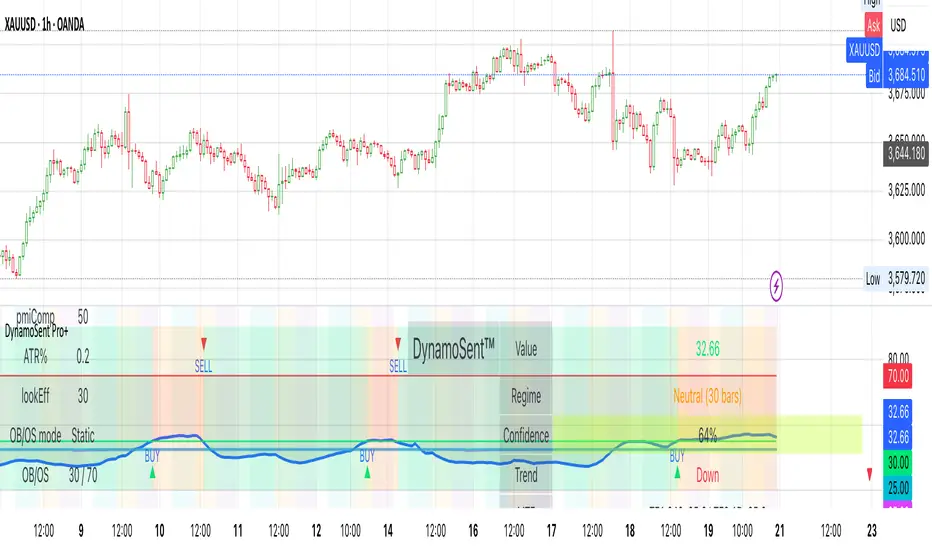
DynamoSent DynamoSent Pro+ — Professional Listing (Preview)
— Adaptive Macro Sentiment (v6)
— Export, Adaptive Lookback, Confidence, Boxes, Heatmap + Dynamic OB/OS
Preview / Experimental build. I’m actively refining this tool—your feedback is gold.
If you spot edge cases, want new presets, or have market-specific ideas, please comment or DM me on TradingView.
⸻
What it is
DynamoSent Pro+ is an adaptive, non-repainting macro sentiment engine that compresses VIX, DXY and a price-based activity proxy (e.g., SPX/sector ETF/your symbol) into a 0–100 sentiment line. It scales context by volatility (ATR%) and can self-calibrate with rolling quantile OB/OS. On top of that, it adds confidence scoring, a plain-English Context Coach, MTF agreement, exportable sentiment for other indicators, and a clean Light/Dark UI.
Why it’s different
• Adaptive lookback tracks regime changes: when volatility rises, we lengthen context; when it falls, we shorten—less whipsaw, more relevance.
• Dynamic OB/OS (quantiles) self-calibrates to each instrument’s distribution—no arbitrary 30/70 lines.
• MTF agreement + Confidence gate reduce false positives by highlighting alignment across timeframes.
• Exportable output: hidden plot “DynamoSent Export” can be selected as input.source in your other Pine scripts.
• Non-repainting rigor: all request.security() calls use lookahead_off + gaps_on; signals wait for bar close.
Key visuals
• Sentiment line (0–100), OB/OS zones (static or dynamic), optional TF1/TF2 overlays.
• Regime boxes (Overbought / Oversold / Neutral) that update live without repaint.
• Info Panel with confidence heat, regime, trend arrow, MTF readout, and Coach sentence.
• Session heat (Asia/EU/US) to match intraday behavior.
• Light/Dark theme switch in Inputs (auto-contrasted labels & headers).
⸻
How to use (examples & recipes)
1) EURUSD (swing / intraday blend)
• Preset: EURUSD 1H Swing
• Chart: 1H; TF1=1H, TF2=4H (default).
• Proxies: Defaults work (VIX=D, DXY=60, Proxy=D).
• Dynamic OB/OS: ON at 20/80; Confidence ≥ 55–60.
• Playbook:
• When sentiment crosses above 50 + margin with Δ ≥ signalK and MTF agreement ≥ 0.5, treat as trend breakout.
• In Oversold with rising Coach & TF agreement, take fade longs back toward mid-range.
• Alerts: Enable Breakout Long/Short and Fade; keep cooldown 8–12 bars.
2) SPY (daytrading)
• Preset: SPY 15m Daytrade; Chart: 15m.
• VIX (D) matters more; preset weights already favor it.
• Start with static 30/70; later try dynamic 25/75 for adaptive thresholds.
• Use Coach: in US session, when it says “Overbought + MTF agree → sell rallies / chase breakouts”, lean momentum-continuation after pullbacks.
3) BTCUSD (crypto, 24/7)
• Preset: BTCUSD 1H; Chart: 1H.
• DXY and BTC.D inform macro tone; keep Carry-forward ON to bridge sparse ticks.
• Prefer Dynamic OB/OS (15/85) for wider swings.
• Fade signals on weekend chop; Breakout when Confidence > 60 and MTF ≥ 1.0.
4) XAUUSD (gold, macro blend)
• Preset: XAUUSD 4H; Chart: 4H.
• Weights tilt to DXY and US10Y (handled by preset).
• Coach + MTF helps separate trend legs from news pops.
⸻
Best practices
• Theme: Switch Light/Dark in Inputs; the panel adapts contrast automatically.
• Export: In another script → Source → DynamoSent Pro+ → DynamoSent Export. Build your own filters/strategies atop the same sentiment.
• Dynamic vs Static OB/OS:
• Static 30/70: fast, universal baseline.
• Dynamic (quantiles): instrument-aware; use 20/80 (default) or 15/85 for choppy markets.
• Confidence gate: Start at 50–60% to filter noise; raise when you want only A-grade setups.
• Adaptive Lookback: Keep ON. For ultra-liquid indices, you can switch it OFF and set a fixed lookback.
⸻
Non-repainting & safety notes
• All request.security() calls use lookahead=barmerge.lookahead_off and gaps=barmerge.gaps_on.
• No forward references; signals & regime flips are confirmed on bar close.
• History-dependent funcs (ta.change, ta.percentile_linear_interpolation, etc.) are computed each bar (not conditionally).
• Adaptive lookback is clamped ≥ 1 to avoid lowest/highest errors.
• Missing-data warning triggers only when all proxies are NA for a streak; carry-forward can bridge small gaps without repaint.
⸻
Known limits & tips
• If a proxy symbol isn’t available on your plan/exchange, you’ll see the NA warning: choose a different symbol via Symbol Search, or keep Carry-forward ON (it defaults to neutral where needed).
• Intraday VIX is sparse—using Daily is intentional.
• Dynamic OB/OS needs enough history (see dynLenFloor). On short histories it gracefully falls back to static levels.
Thanks for trying the preview. Your comments drive the roadmap—presets, new proxies, extra alerts, and integrations.
Multi-Indicator Panel (RSI, Stoch, MACD, VIX Fix, MFI)A versatile single-pane oscillator panel combining RSI, Stochastic, MACD (scaled to 0–100), Williams VIX Fix (normalized & inverted: low value = high fear), and MFI. Each module is toggleable, with reference levels, background highlights, and ready-made alerts.
Key features
Per-indicator toggles: RSI, Stoch %K/%D, MACD (lines + optional histogram), inverted 0–100 VIX Fix, and MFI.
Standard levels & center line at 50; adjustable overbought/oversold thresholds.
Contextual background coloring (optional) for extreme conditions.
Built-in alerts: RSI/Stoch OB/OS, MACD–Signal cross, VIX Fix “High Fear/Low Fear,” and MFI OB/OS.
Unified scale: MACD mapped around 50 to align with other oscillators; VIX Fix normalized to 0–100.
How to use (quick)
Add the indicator → enable needed modules via “Indicator Toggles.”
Tune periods & levels (e.g., RSI 14, Stoch 14/3, MACD 12-26-9, VIX Fix 22/252, MFI 14).
(Optional) Turn on MACD histogram.
Create alerts from “Add alert on…” using the provided conditions.
Interpretation notes
Inverted VIX Fix: low values ⇒ high fear/volatility (potential bounces); high values ⇒ complacency.
Scaled MACD: lines around 50 ≈ MACD zero; line crosses remain valid despite scaling.
Disclaimer
Analysis tool, not financial advice. Test across timeframes/instruments and pair with risk management.

Advanced Trading System - [WOLONG X DBG]Advanced Multi-Timeframe Trading System
Overview
This technical analysis indicator combines multiple established methodologies to provide traders with market insights across various timeframes. The system integrates SuperTrend analysis, moving average clouds, MACD-based candle coloring, RSI analysis, and multi-timeframe trend detection to suggest potential entry and exit opportunities for both swing and day trading approaches.
Methodology
The indicator employs a multi-layered analytical approach based on established technical analysis principles:
Core Signal Generation
SuperTrend Engine: Utilizes adaptive SuperTrend calculations with customizable sensitivity (1-20) combined with SMA confirmation filters to identify potential trend changes and continuations
Braid Filter System: Implements moving average filtering using multiple MA types (McGinley Dynamic, EMA, DEMA, TEMA, Hull, Jurik, FRAMA) with percentage-based strength filtering to help reduce false signals
Multi-Timeframe Analysis: Analyzes trend conditions across 10 different timeframes (1-minute to Daily) using EMA-based trend detection for broader market context
Advanced Features
MACD Candle Coloring: Applies dynamic 4-level candle coloring system based on MACD histogram momentum and signal line relationships for visual trend strength assessment
RSI Analysis: Identifies potential reversal areas using RSI oversold/overbought conditions with SuperTrend confirmation
Take Profit Analysis: Features dual-mode TP detection using statistical slope analysis and Parabolic SAR integration for exit timing analysis
Key Components
Signal Types
Primary Signals: Green ▲ for potential long entries, Red ▼ for potential short entries with trend and SMA alignment
Reversal Signals: Small circular indicators for RSI-based counter-trend possibilities
Take Profit Markers: X-cross symbols indicating statistical TP analysis zones
Pullback Signals: Purple arrows for potential trend continuation entries using Parabolic SAR
Visual Elements
8-Layer MA Cloud: Customizable moving average cloud system with 3 color themes for trend visualization
Real-Time Dashboard: Multi-timeframe trend analysis table showing bullish/bearish status across all timeframes
Dynamic Candle Colors: 4-intensity MACD-based coloring system (ranging from light to strong trend colors)
Entry/SL/TP Labels: Automatic calculation and display of suggested entry points, stop losses, and multiple take profit levels
Usage Instructions
Basic Configuration
Sensitivity Setting: Start with default value 6
Increase (7-15) for more frequent signals in volatile markets
Decrease (3-5) for higher quality signals in trending markets
MA Filter Type: McGinley Dynamic recommended for smoother signals
Filter Strength: Set to 80% for balanced filtering, adjust based on market conditions
Signal Interpretation
Long Entry: Green ▲ suggests when price crosses above SuperTrend with bullish SMA alignment
Short Entry: Red ▼ suggests when price crosses below SuperTrend with bearish SMA alignment
Reversal Opportunities: Small circles indicate RSI-based counter-trend analysis
Take Profit Zones: X-crosses mark statistical TP areas based on slope analysis
Dashboard Analysis
Green Cells: Bullish trend detected on that timeframe
Red Cells: Bearish trend detected on that timeframe
Multi-Timeframe Confluence: Look for alignment across multiple timeframes for stronger signal confirmation
Risk Management Features
Automatic Calculations
ATR-Based Stop Loss: Dynamic stop loss calculation using ATR multiplier (default 1.9x)
Multiple Take Profit Levels: Three TP targets with 1:1, 1:2, and 1:3 risk-reward ratios
Position Sizing Guidance: Entry labels display suggested price levels for order placement
Confirmation Requirements
Trend Alignment: Requires SuperTrend and SMA confirmation before signal generation
Filter Validation: Braid filter must show sufficient strength before signals activate
Multi-Timeframe Context: Dashboard provides broader market context for decision making
Optimal Settings
Timeframe Recommendations
Scalping: 1M-5M charts with sensitivity 8-12
Day Trading: 15M-1H charts with sensitivity 6-8
Swing Trading: 4H-Daily charts with sensitivity 4-6
Market Conditions
Trending Markets: Reduce sensitivity, increase filter strength
Ranging Markets: Increase sensitivity, enable reversal signals
High Volatility: Adjust ATR risk factor to 2.0-2.5
Advanced Features
Customization Options
MA Cloud Periods: 8 customizable periods for cloud layers (default: 2,6,11,18,21,24,28,34)
Color Themes: Three professional color schemes plus transparent option
Dashboard Position: 9 positioning options with 4 size settings
Signal Filtering: Individual toggle controls for each signal type
Technical Specifications
Moving Average Types: 21 different MA calculations including advanced types (Jurik, FRAMA, VIDA, CMA)
Pullback Detection: Parabolic SAR with customizable start, increment, and maximum values
Statistical Analysis: Linear regression slope calculation for trend-based TP analysis
Important Limitations
Lagging Nature: Some signals may appear after potential entry points due to confirmation requirements
Ranging Markets: May produce false signals during extended sideways price action
High Volatility: Requires parameter adjustment during news events or unusual market conditions
Computational Load: Multiple timeframe analysis may impact performance on slower devices
No Guarantee: All signals are suggestions based on technical analysis and may be incorrect
Educational Disclaimers
This indicator is designed for educational and analytical purposes only. It represents a technical analysis tool based on mathematical calculations of historical price data and should not be considered as financial advice or trading recommendations.
Risk Warning: Trading involves substantial risk of loss and is not suitable for all investors. Past performance of any trading system or methodology is not necessarily indicative of future results. The high degree of leverage can work against you as well as for you.
Important Notes:
Always conduct your own analysis before making trading decisions
Use appropriate position sizing and risk management strategies
Never risk more than you can afford to lose
Consider your investment objectives, experience level, and risk tolerance
Seek advice from qualified financial professionals when needed
Performance Disclaimer: Backtesting results do not guarantee future performance. Market conditions change constantly, and what worked in the past may not work in the future. Always paper trade new strategies before risking real capital.
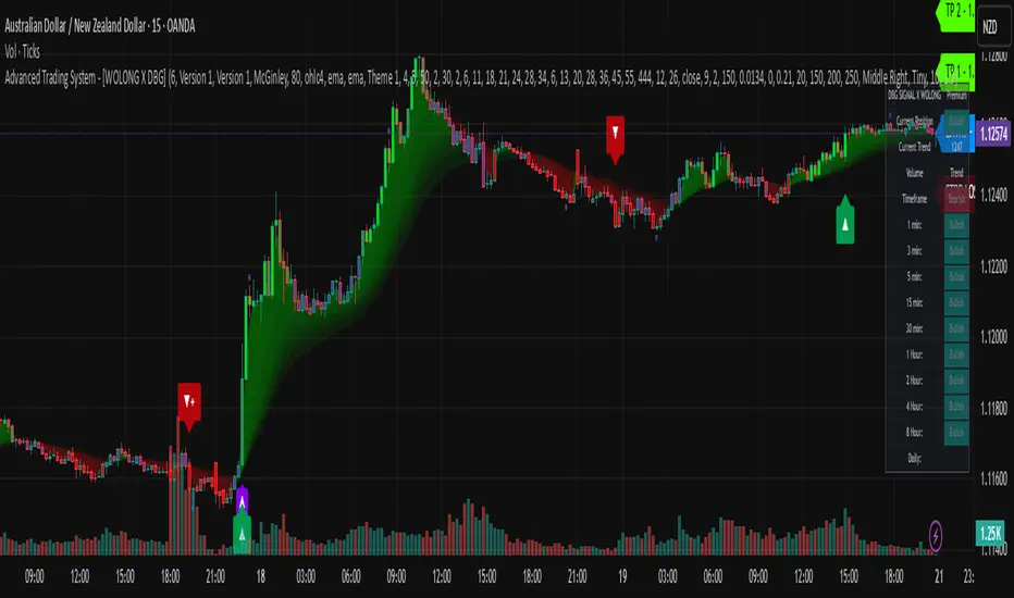
Profit Filter RSI+MACD//@version=5
indicator("Profit Filter RSI+MACD", overlay=true)
// Trend filter
ema200 = ta.ema(close, 200)
// RSI
rsi = ta.rsi(close, 14)
// MACD
macd = ta.ema(close,12) - ta.ema(close,26)
signal = ta.ema(macd,9)
// Long signal
longCond = close > ema200 and rsi < 30 and ta.crossover(macd, signal)
// Short signal
shortCond = close < ema200 and rsi > 70 and ta.crossunder(macd, signal)
// Plot signals
plotshape(longCond, title="Long Entry", location=location.belowbar,
color=color.green, style=shape.labelup, text="LONG")
plotshape(shortCond, title="Short Entry", location=location.abovebar,
color=color.red, style=shape.labeldown, text="SHORT")
// Plot EMA
plot(ema200, "EMA 200", color=color.orange)

EMRVA//@version=5
indicator("EMRVA", overlay=true)
// === الإعدادات ===
emaLength = input.int(200, "EMA Length")
rsiLength = input.int(14, "RSI Length")
volLength = input.int(20, "Volume MA Length")
adxLength = input.int(14, "ADX Length")
adxFilter = input.int(20, "ADX Minimum Value") // فلتر الاتجاه
// === EMA200 ===
ema200 = ta.ema(close, emaLength)
plot(ema200, color=color.orange, linewidth=2, title="EMA 200")
// === MACD ===
macdLine = ta.ema(close, 12) - ta.ema(close, 26)
signalLine = ta.ema(macdLine, 9)
// === RSI ===
rsi = ta.rsi(close, rsiLength)
// === Volume Confirmation ===
volMA = ta.sma(volume, volLength)
volCond = volume > volMA
// === ADX Manual Calculation ===
upMove = high - high
downMove = low - low
plusDM = na(upMove) ? na : (upMove > downMove and upMove > 0 ? upMove : 0)
minusDM = na(downMove) ? na : (downMove > upMove and downMove > 0 ? downMove : 0)
tr = ta.rma(ta.tr, adxLength)
plusDI = 100 * ta.rma(plusDM, adxLength) / tr
minusDI = 100 * ta.rma(minusDM, adxLength) / tr
dx = 100 * math.abs(plusDI - minusDI) / (plusDI + minusDI)
adx = ta.rma(dx, adxLength)
adxCond = adx > adxFilter
// === شروط الدخول والخروج ===
longCond = close > ema200 and macdLine > signalLine and rsi > 50 and volCond and adxCond
shortCond = close < ema200 and macdLine < signalLine and rsi < 50 and volCond and adxCond
// === منطق الإشارة عند بداية الاتجاه فقط ===
var inLong = false
var inShort = false
buySignal = longCond and not inLong
sellSignal = shortCond and not inShort
if buySignal
inLong := true
inShort := false
if sellSignal
inShort := true
inLong := false
// === إشارات ثابتة ===
plotshape(buySignal, title="Buy Signal", location=location.belowbar,
color=color.green, style=shape.labelup, text="BUY")
plotshape(sellSignal, title="Sell Signal", location=location.abovebar,
color=color.red, style=shape.labeldown, text="SELL")
// === تنبيهات ===
alertcondition(buySignal, title="Buy Alert", message="📈 إشارة شراء مؤكدة مع فلتر ADX")
alertcondition(sellSignal, title="Sell Alert", message="📉 إشارة بيع مؤكدة مع فلتر ADX")
// === رسم ADX للتأكيد ===
plot(adx, title="ADX", color=color.blue)
hline(adxFilter, "ADX Filter", color=color.red)

EMRV101//@version=5
indicator("EMA200 + MACD + RSI + Volume Confirmation + Alerts", overlay=true)
// === الإعدادات ===
emaLength = input.int(200, "EMA Length")
rsiLength = input.int(14, "RSI Length")
volLength = input.int(20, "Volume MA Length")
// === EMA200 ===
ema200 = ta.ema(close, emaLength)
plot(ema200, color=color.orange, linewidth=2, title="EMA 200")
// === MACD ===
macdLine = ta.ema(close, 12) - ta.ema(close, 26)
signalLine = ta.ema(macdLine, 9)
// === RSI ===
rsi = ta.rsi(close, rsiLength)
// === Volume Confirmation ===
volMA = ta.sma(volume, volLength)
volCond = volume > volMA
// === شروط الدخول والخروج ===
longCond = close > ema200 and macdLine > signalLine and rsi > 50 and volCond
shortCond = close < ema200 and macdLine < signalLine and rsi < 50 and volCond
// === منطق الإشارة عند بداية الاتجاه فقط ===
var inLong = false
var inShort = false
buySignal = longCond and not inLong
sellSignal = shortCond and not inShort
if buySignal
inLong := true
inShort := false
if sellSignal
inShort := true
inLong := false
// === إشارات ثابتة ===
plotshape(buySignal, title="Buy Signal", location=location.belowbar,
color=color.green, style=shape.labelup, text="BUY")
plotshape(sellSignal, title="Sell Signal", location=location.abovebar,
color=color.red, style=shape.labeldown, text="SELL")
// === تنبيهات ===
alertcondition(buySignal, title="Buy Alert", message="📈 إشارة شراء مؤكدة")
alertcondition(sellSignal, title="Sell Alert", message="📉 إشارة بيع مؤكدة")

MACD Scaled Overlay█ OVERVIEW
The "MACD Scaled Overlay" indicator is an advanced version of the classic MACD (Moving Average Convergence Divergence) oscillator that displays signals directly on the price chart. Instead of a traditional separate panel, the MACD line, signal line, and histogram are scaled and overlaid on the price chart, making it easier to identify key price levels and potential reversal points. The indicator also supports the detection of divergences (regular and hidden) and offers extensive customization options, such as adjusting colors, line thickness, and enabling/disabling visual elements.
█ CONCEPTS
The "MACD Scaled Overlay" indicator is designed to simplify trend and reversal analysis by integrating MACD signals with the price chart. The MACD Scaled Overlay is scaled relative to the average candle range, allowing the lines and histogram to dynamically adjust to market volatility. Additionally, the indicator enables the detection of divergences (bullish and bearish, both regular and hidden) based on the traditional MACD histogram (before scaling), ensuring consistency with classic divergence analysis. The indicator is most effective when combined with other technical analysis tools, such as Fibonacci levels, pivot points, or trend lines.
█ MACD Calculations and Scaling
The indicator is based on the classic MACD formula, which includes:
-MACD Line: The difference between the fast EMA (default: 12) and the slow EMA (default: 26).
-Signal Line: The EMA of the MACD line (default: 9).
-Histogram: The difference between the MACD line and the signal line.
Scaling is achieved by normalizing the MACD values relative to the standard deviation and the average candle range. This makes the lines and histogram dynamically adjust to market volatility, improving their readability and utility on the price chart. The scaling formulas are:
-MACD Scaled: macdNorm * avgRangeLines * scaleFactor
-Signal Scaled: signalNorm * avgRangeLines * scaleFactor
-Histogram Scaled: histNorm * avgRangeHist * scaleFactor
Where:
-macdNorm and signalNorm are the normalized MACD and signal line values.
-avgRangeLines and avgRangeHist are the average candle ranges.
-scaleFactor is the scaling multiplier (default: 2).
The positioning of the lines and histogram is relative to the candle midpoint (candleMid = (high + low) / 2), ensuring proper display on the price chart. Divergences are calculated based on the traditional MACD histogram (before scaling), maintaining consistency with standard divergence detection methodology.
█INDICATOR FEATURES
-Dynamic MACD and Signal Lines: Scaled and overlaid on the price chart, facilitating the identification of reversal points.
-Histogram: Displays the difference between the MACD and signal lines, dynamically adjusted to market volatility.
-Divergence Detection: Ability to detect regular and hidden divergences (bullish and bearish) based on the traditional MACD histogram, with options to enable/disable their display.
-Visual Customization: Options to adjust colors, line thickness, transparency, and enable/disable elements such as the zero line, MACD line, signal line, or histogram.
-Smoothing: Smoothing length for lines (default: 1) and histogram (default: 3). Smoothing may delay crossover signals, which should be considered during analysis.
-Alerts: Alert conditions for MACD and signal line crossovers, enabling notifications for potential buy/sell signals.
█ HOW TO SET UP THE INDICATOR
-Add the "MACD Scaled Overlay" indicator to your TradingView chart.
-Configure parameters in the settings, such as EMA lengths, scaling multiplier, or smoothing periods, to match your trading style.
-Enable or disable the display of the zero line, MACD line, signal line, or histogram based on your needs.
-Adjust colors and line thickness in the "Style" section and transparency settings in the input section to optimize visualization.
█ HOW TO USE
Add the indicator to your chart, configure the parameters, and observe the interactions of the price with the MACD line, signal line, and histogram to identify potential entry and exit points. Key signals include:
-MACD and Signal Line Crossovers: A crossover of the MACD line above the signal line may indicate a buy signal (bullish cross), while a crossover below the signal line may indicate a sell signal (bearish cross).
-Crossings Through the Price Line (Zero): The MACD line or histogram crossing the price line (candle midpoint) may indicate a change in momentum. For example, the histogram moving from negative to positive values near the price line may signal increasing bullish trend strength.
-Divergences: Detection of regular and hidden divergences (bullish and bearish) based on the traditional MACD histogram can help predict trend reversals. Divergences are not standalone signals, as they are delayed by the specified pivot length (default: 3). However, they help strengthen the significance of other signals, such as crossovers or support/resistance levels.
The indicator is most effective when combined with other tools, such as Fibonacci levels, pivot points, or support/resistance lines, to confirm signals.
