Forex Dynamic Lot Size CalculatorForex Dynamic Lot Size Calculator for Forex. Works on USD Base and USD Quote pairs. Provides real-time data based on stop-loss location. Allows you to know in real-time how the number of lots you need to purchase to match your risk %.
Number of Lots is calculated based on total risk. Total risk is calculated based on Stop-Loss + Commission + Spread Fees + Slippage measured in pips. Also includes data such as break-even pips, net take profit, margin required, buying power used, and a few others. All are real-time and anchored to the current price.
The intention of creating this indicator is to help with risk management. You know exactly how many lots you need to get this very moment to have your total risk at lets say $250, which includes commission fees, spread fees, and slippage.
To put it simply, if I was to enter the trade right now and willing to risk exactly $250, how many lots will I need to get right this second?
---
- To use adjust Account Settings along with other variables.
- Stop Loss Mode can be Manual or Dynamic. If you select Dynamic, then you will have to adjust Stop Loss Level to where you can see the reference line on the screen. It is at 1.1 by default. Just enter current price and the line will appear. Adjust it by dragging it to where you want your stop loss to be.
- Take Profit Mode can also be Manual or Dynamic. I just keep my TP at Manual and use Quick Access to set Quick RR levels.
- Adjust Spreads and Slippage to your liking. I tried to have TV calculate current spread, but it seem like it doesn't have access to real-life data for me like MT5 does. I just use average instead. Both are optional, depending on your broker and type of account you use.
- Pip Value for the current pair, Return on Margin, and Break-even line can be turned on and off, based on your needs. I just get the Break-even value in pips from the pannel and use that as reference where I need to relocate my stop loss to break-ever (commission + spreds + slippage).
- Panel is fully customizable based on your liking. Important fields are highlighted along with reference lines.
Statistics

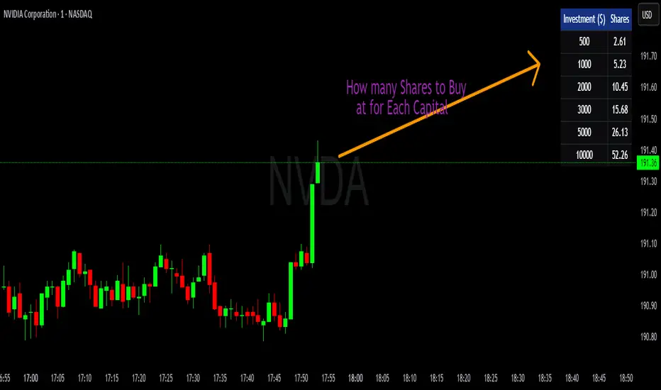
💰 Position Size Table Compact Quickly see how many shares you can buy for preset investment amounts at the current price. This compact, customizable table is perfect for traders who want to calculate position sizes instantly without manual math.
Features
- Pre-set investment amounts: $500, $1000, $2000, $3000, $5000, $10000
- Per-row toggle: Show or hide specific investment amounts
- Live updates: Table recalculates as the stock price changes
- Customizable colors: Background, header, text, and border
- Master toggle: Hide or show the entire table on demand
Use it to
- Quickly calculate position sizes for multiple investment levels
- Plan trades efficiently and reduce manual calculation errors
- Keep your chart clean with a compact, flexible table
Signature [Pro+]Signature - Release
Indicator Table Features:
- Customizable indicator title display
- Real-time clock with timezone support
- 12-hour or 24-hour time format options
- Toggle AM/PM display for 12-hour format
- Individual text size control for clock
- Ticker symbol display
- Timeframe display
- Flexible table positioning (9 positions available)
- Customizable text colors, background colors, and border colors
- Font family selection (Default or Monospace)
- Individual control to enable/disable each element
- Text alignment control (Left, Center, Right)
Watermark Table Features:
- Customizable header text
- Customizable subtitle text
- Current date display with multiple format options
- Date month format: Full, Abbreviated, or Number
- Date year format: Full or Abbreviated
- Date separator options: dot, slash, dash, or space
- Flexible table positioning (9 positions available)
- Customizable text colors, background colors, and border colors
- Font family selection (Default or Monospace)
- Individual control to enable/disable each element
- Text alignment control (Left, Center, Right)
General Features:
- Two independent tables that can be positioned anywhere
- All styling consistent across both tables
- Minimal and clean design
- No performance impact on chart analysis
- Text alignment options for both indicator and watermark tables

Psychological Levels + Retest The script detects key round-number psychological levels such as 00, 50, and 100 zones based on the pair’s pip structure.
It then monitors price behavior around these zones using customizable buffers to highlight reaction areas.
When price breaks above a major or minor psychological level while trading above the 200 EMA, the indicator tracks for a retest confirmation. Once the required number of touches occurs within the defined buffer, the indicator marks the retest area and can trigger alerts for trade opportunities.

Auto Option Premium Viewer - csgnanamThat's a great idea! Clear documentation is key for anyone using your script. Since your selected code block is the dedicated space for documentation, I'll provide an explanation tailored for that context, covering the main features of your "Auto Option Premium Viewer" Canvas.
Here is a detailed explanation of the script's core functionality, which you can use in your Canvas description or in a separate document to help users understand it.
I will not edit the Canvas itself, as you requested a separate explanation.
***
### Explanation of the "Auto Option Premium Viewer" Canvas
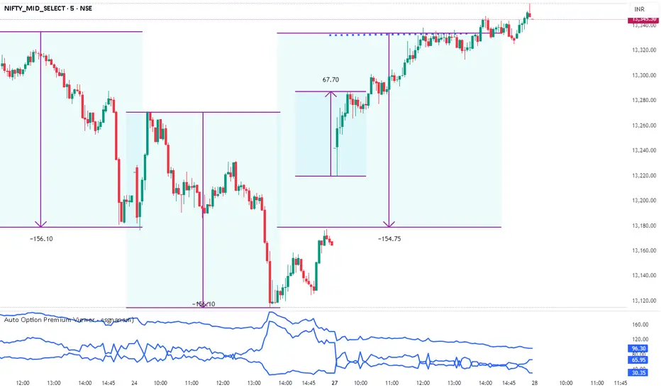
This Pine Script indicator, **"Auto Option Premium Viewer — Full Auto Symbols (NSE format, improved detection),"** is designed to automatically fetch and display the At-The-Money (ATM) Call and Put option premiums for major NSE indices (NIFTY, BANKNIFTY, MIDCPNIFTY, FINNIFTY) in real-time.
The primary goal is to provide a single, clean chart overlay showing the total premium (CE + PE) for the options closest to the current spot price, without requiring the user to manually enter strike prices or steps.
#### 1. Automatic Index Detection (`AUTO` Functionality)
* **Smart Underlying Detection:** The script attempts to automatically detect the index you are currently viewing (`activeUnderlying`). For example, if your chart is set to `BANKNIFTY`, the indicator automatically focuses on Bank Nifty options.
* **Spot Ticker Mapping (The Fix):** To accurately find the spot price, the script uses a helper function (`getSpotTicker`) to map the common index name (like `FINNIFTY`) to the specific underlying ticker required by TradingView (like `CNXFINANCE` or `NIFTY_MID_SELECT`). This ensures accurate price referencing for ATM calculation across all indices.
#### 2. Fully Automated Strike & Step Sizing
* **No Base Strike Inputs:** The script dynamically calculates the At-The-Money (ATM) strike price based on the live spot price of the underlying index.
* **Fixed Strike Steps:** The strike increment (`current_step`) is hardcoded based on market conventions:
* **100:** NIFTY, BANKNIFTY, FINNIFTY
* **50:** MIDCPNIFTY
* **Dynamic ATM Calculation:** The live spot price is rounded to the nearest valid strike based on the correct step size. This automatically determines the central strike (B), along with the adjacent strikes (A and C) to ensure the fetched data is always relevant.
#### 3. Data Fetching and Display
* **Symbol Construction:** The `buildSymbol` function creates the exact NSE option symbol string (e.g., `NSE:NIFTY251028C26000`) required by the `request.security` function.
* **Option Price Request:** The script uses `request.security` to fetch the closing price (`close`) of the Call and Put options for the three relevant strikes (A, B, C) on a fixed **5-minute** timeframe (`dataTF`).
* **Plots:** The indicator displays three lines on the chart's lower panel:
1. **ATM CE Premium:** The price of the Call option closest to ATM.
2. **ATM PE Premium:** The price of the Put option closest to ATM.
3. **ATM Total Premium:** The sum of CE + PE, often used as a proxy for the minimum expected range or implied volatility.
This automatic setup makes the Canvas extremely efficient for quick analysis without needing to manually adjust any numerical settings.
Risk Leverage ToolRisk Leverage Tool – Calculate Position Size and Required Leverage
This script automatically calculates the optimal position size and the leverage needed based on the amount of capital you are willing to risk on a trade. It is designed for traders who want precise control over their risk management.
The script determines the distance between the entry and stop-loss price, calculates the maximum position size that fits within the defined risk, and derives the notional value of the trade. Based on the available margin, it then calculates the required leverage. It also displays the percentage of margin at risk if the stop-loss is hit.
All results are displayed in a table in the top-right corner of the chart. Additionally, a label appears at the entry price level showing the same data.
To use the tool, simply input your planned entry price, stop-loss price, the maximum risk amount in dollars, and the available margin in the settings menu. The script will update all values automatically in real time.
This tool works with any market where capital risk is expressed in absolute terms (such as USD), including futures, CFDs, and leveraged spot positions. For inverse contracts or percentage-based stops, manual adjustment is required.

Adaptive Trend SelectorThe Adaptive Trend Selector is a comprehensive trend-following tool designed to automatically identify the optimal moving average crossover strategy. It features adjustable parameters and an integrated backtester that delivers institutional-grade insights into the recommended strategy. The model continuously adapts to new data in real time by evaluating multiple moving average combinations, determining the best performing lengths, and presenting the backtest results in a clear, color-coded table that benchmarks performance against the buy-and-hold strategy.
At its core, the model systematically backtests a wide range of moving average combinations to identify the configuration that maximizes the selected optimization metric. Users can choose to optimize for absolute returns or risk-adjusted returns using the Sharpe, Sortino, or Calmar ratios. Alternatively, users can enable manual optimization to test custom fast and slow moving average lengths and view the corresponding backtest results. The label displays the Compounded Annual Growth Rate (CAGR) of the strategy, with the buy-and-hold CAGR in parentheses for comparison. The table presents the backtest results based on the fast and slow lengths displayed at the top:
Sharpe = CAGR per unit of standard deviation.
Sortino = CAGR per unit of downside deviation.
Calmar = CAGR relative to maximum drawdown.
Max DD = Largest peak-to-trough decline in value.
Beta (β) = Return sensitivity relative to buy-and-hold.
Alpha (α) = Excess annualized risk-adjusted returns.
Win Rate = Ratio of profitable trades to total trades.
Profit Factor = Total gross profit per unit of losses.
Expectancy = Average expected return per trade.
Trades/Year = Average number of trades per year.
This indicator is designed with flexibility in mind, enabling users to specify the start date of the backtesting period and the preferred moving average strategy. Supported strategies include the Exponential Moving Average (EMA), Simple Moving Average (SMA), Wilder’s Moving Average (RMA), Weighted Moving Average (WMA), and Volume-Weighted Moving Average (VWMA). To minimize overfitting, users can define constraints such as a minimum and maximum number of trades per year, as well as an optional optimization margin that prioritizes longer, more robust combinations by requiring shorter-length strategies to exceed this threshold. The table follows an intuitive color logic that enables quick performance comparison against buy-and-hold (B&H):
Sharpe = Green indicates better than B&H, while red indicates worse.
Sortino = Green indicates better than B&H, while red indicates worse.
Calmar = Green indicates better than B&H, while red indicates worse.
Max DD = Green indicates better than B&H, while red indicates worse.
Beta (β) = Green indicates better than B&H, while red indicates worse.
Alpha (α) = Green indicates above 0%, while red indicates below 0%.
Win Rate = Green indicates above 50%, while red indicates below 50%.
Profit Factor = Green indicates above 2, while red indicates below 1.
Expectancy = Green indicates above 0%, while red indicates below 0%.
In summary, the Adaptive Trend Selector is a powerful tool designed to help investors make data-driven decisions when selecting moving average crossover strategies. By optimizing for risk-adjusted returns, investors can confidently identify the best lengths using institutional-grade metrics. While results are based on the selected historical period, users should be mindful of potential overfitting, as past results may not persist under future market conditions. Since the model recalibrates to incorporate new data, the recommended lengths may evolve over time.

Market Screener - NarwingThis is a 20 cryptocurrency market screener, it's goal is to provide a broad view of the state of cryptocurrencies using 4 key components
1. ROC
2. Sharpe Ratio
3. Sortino Ratio
4. Omega Ratio
All these metrics are calculated twice with two different lengths, 7 day and 30 days
This allows for broad market screening instead of focusing on one particular asset
This tool is meant for research purposes only, never invest money you can't afford to lose

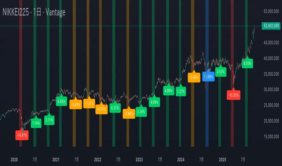
Mercury Retrograde — Daily boxes & bottom % (stable v6)水星逆行のアノマリー検証。対象は日経225の過去5年の値動き。水星逆行開始時の終値と水星逆行終了時の終値を比較。上昇率・下落率に応じて色分け。
Verification of Mercury Retrograde Anomalies. Subject: Nikkei 225 price movements over the past five years. Comparing closing prices at the start and end of Mercury retrograde periods. Color-coded based on percentage increase/decrease.
The Wick Report [Pro]Overview
The Wick Report visualizes how current wick development compares to long-term statistical behavior across multiple higher-timeframe candles.
It references embedded datasets to show where wick formation is historically common, rare, or unusually small for a given session or timeframe.
This provides a data-driven context for directional bias and wick-based targeting — without implying any form of prediction.
Candles that form little or no wick are statistically uncommon. The Wick Report highlights these conditions and displays their percentile rank, exceedance probability, and a derived “score” that reflects how far current wick behavior deviates from typical norms.
Key Features
• Multi-Timeframe Analysis – View wick statistics from 4H, 6H, 12H, Daily, or Weekly candles projected onto any chart.
• Wick Probabilities – Quantifies the historical likelihood of a wick extending beyond its current size.
• Percentile Mapping – Shows where each wick sits within its long-term distribution (e.g., P25 = smaller than 75 % of prior wicks).
• Score System – Automatically combines percentile and probability into a single normalized “target score” for simplified interpretation.
• Wick Modes – Choose how wick data is displayed to suit your analysis style:
– Auto — Detects candle direction automatically and draws the statistically relevant wick (upper or lower).
– Bullish Only — Displays only lower wicks from bullish candles.
– Bearish Only — Displays only upper wicks from bearish candles.
– Both — Draws both upper and lower wick zones simultaneously for full candle symmetry.
• Adaptive Visualization – Color-coded zones and dynamic labels update as higher-timeframe candles evolve.
• Threshold Filters – Optional probability or score filters to hide low-significance wicks.
About the Score
The score balances two opposing factors:
• High probability of a wick extending further, and
• Low percentile ranking (a smaller-than-normal wick).
A strong combination of both produces a higher score, highlighting candles where wick development is statistically most imbalanced.
The scale is purely comparative — derived from historical distributions, not forward prediction.
Target Score Rankings
Outstanding (70 +) – Extremely rare, high-confidence zones — typically at very low percentiles with strong exceedance probability.
Excellent (60–70) – High-confidence targets with clear statistical edge.
Good (50–60) – Solid probability zones, reliable reference levels.
Above Average (40–50) – Decent opportunities within normal ranges.
Average (30–40) – Neutral zones; use additional confirmation.
Below Average (20–30) – Low-confidence references.
Poor (< 20) – High percentiles with low probability; statistically common and uninformative.
Methodology & Use
The Wick Report uses historical wick distributions to classify how current wick sizes compare to typical behavior for the same timeframe and session hour.
When a candle forms a small or missing wick, the tool reports how often that condition historically remained unchanged through the rest of the candle’s interval.
This helps identify when wick development is statistically under- or over-extended.
The data is intended for contextual reference only — for example, combining a high-score, low-percentile wick on a higher timeframe with lower-timeframe structure may provide useful directional confluence.
It does not generate trade signals or predict future movement.
Proprietary Framework
The Wick Report uses embedded statistical datasets built from more than a decade of historical market behavior.
Each timeframe references pre-processed wick-size and exceedance distributions to display where the current wick sits within its long-term statistical range.
All computational methods and dataset structures remain proprietary.

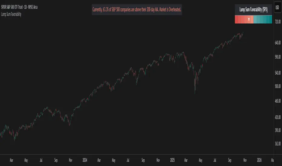
Lump Sum Favorability (SPX & NDX)This indicator provides a visual dashboard to gauge the statistical favorability of deploying a "Lump Sum" investment into the SPX (S&P 500) or NDX (Nasdaq 100).
The primary goal is not to time the exact market bottom, but to identify zones of significant pessimism or euphoria. Historically, periods of indiscriminate selling have represented high-probability entry points for long-term investors.
The dashboard consists of two parts:
1. The Favorability Gauge: A 12-segment gauge that moves from Red (Unfavorable) to Teal (Favorable).
2. The Summary Text: An optional text box (enabled in settings) that provides a plain-English summary of the current market breadth.
---
The Method: Market Breadth
This indicator is not based on the price of the index itself. Price-based indicators (like an RSI on the SPX) can be misleading. In a market-cap-weighted index, a few mega-cap stocks can hold the index price up while the vast majority of "average" stocks are already in a deep bear market.
This tool uses Market Breadth to measure the true, underlying health and participation of the entire market.
How It Works
1. Data Source: The indicator pulls the daily percentage of companies within the selected index (SPX or NDX) that are trading above their 200-day moving average. (Data tickers: S5TH for SPX, NDTH for NDX).
2. Smoothing: This raw data is volatile. To filter out daily noise and confirm a persistent trend, the indicator calculates a 5-day Simple Moving Average (SMA) of this percentage. This is the value used by the indicator.
3. Interpretation:
High Value (>= 50%): More than half of the stocks are above their long-term average. This signifies the market is "Overheated" or in a risk-on phase. The favorability for a new lump sum investment is considered Low.
Low Value (< 50%): Less than half of the stocks are above their long-term average. This signifies "Oversold" conditions or capitulation. These moments historically offer the best favorability for starting a new long-term investment.
---
How to Use the Indicator
1. The Favorability Gauge
The gauge is designed to be intuitive: Red means "Stop/Caution," and Teal means "Go/Opportunity."
Note: The gauge's logic is inverted from the data value to achieve this simplicity.
Red Zone (Left): UNFAVORABLE
This corresponds to a high percentage of stocks being above their 200d MA (>= 50%). The market is considered Overheated, and the favorability for a new lump sum investment is low.
Teal Zone (Right): FAVORABLE
This corresponds to a low percentage of stocks being above their 200d MA (< 50%). The market is considered Oversold, and the favorability for a new lump sum investment is high.
2. The Summary Text
When "Show Summary Text" is enabled in the settings, a box will appear at the top-center of your chart. This box provides a clear, data-driven summary, such as:
"Currently, only 22% of S&P 500 companies are above their 200-day MA. Market is Oversold."
The color of this text will automatically change to match the market state (Red for Overheated, Teal for Oversold), providing instant confirmation of the gauge's reading.
---
Settings
Market: Choose the index to analyze: SPX (S&P 500) or NDX (Nasdaq 100).
Gauge Position: Select where the gauge dashboard should appear on your chart (default is Bottom Right).
Show Summary Text: Toggle the descriptive text box on or off (default is On).
---
This indicator is a statistical and historical guide, not a financial advice or timing signal. It is designed to measure favorability based on past market behavior, not to provide certainty.
Extreme oversold conditions can persist, and markets can always go lower. This tool should be used as one component of a broader investment and risk-management framework. Past performance is not a guarantee of future results.
GARCH Range PredictorThis was inspired by deltatrendtrading's video on GARCH models to predict daily trading ranges and identify favorable trading conditions. Based on advanced volatility forecasting techniques, it predicts whether a trading day's true range will exceed a threshold, helping traders decide when to trade or skip a session.
Key Features
GARCH(1,1) Volatility Modeling: Uses log-transformed true ranges with exponential moving average centering
Forward-Looking Predictions: Makes predictions at session start before the day unfolds
Dynamic or Static Thresholds: Choose between fixed dollar thresholds or adaptive 20-day averages
Accuracy Tracking: Monitors prediction accuracy with overall and recent (20-day) hit rates
Visual Session Boxes: Colors trading sessions green (trade) or red (skip) based on predictions
Real-Time Statistics: Displays current predictions, thresholds, and performance metrics
How It Works
Data Transformation: Log-transforms daily true ranges and centers them using an EMA
Variance Modeling: Updates GARCH variance using: σ²ₜ = ω + α(residual²) + β(σ²ₜ₋₁)
Prediction Generation: Back-transforms log predictions to dollar values
Signal Generation: Compares predictions to threshold to generate trade/skip signals
Performance Tracking: Validates predictions against actual outcomes
Parameters
GARCH Parameters (ω, α, β): Control volatility persistence and mean reversion
EMA Period: Smoothing period for log range centering
Threshold Settings: Static dollar amount or dynamic multiplier of recent averages
Session Time: Define regular trading hours for analysis
Best Use Cases
Breakout and momentum strategies that perform better on high-range days
Risk management by avoiding low-volatility sessions
Futures day trading (optimized for MNQ/NQ detection)
Any strategy where daily range impacts profitability
Important Notes
Requires 5+ sessions for initialization and warm-up
Accuracy depends heavily on proper parameter tuning for your specific instrument
Default parameters may need adjustment for different markets
Monitor the hit rate to validate effectiveness on your timeframe

RBLR - GSK Vizag AP IndiaThis indicator identifies the Opening Range High (ORH) and Low (ORL) based on the first 15 minutes of the Indian equity market session (9:15 AM to 9:30 AM IST). It draws horizontal lines extending these levels until market close (3:30 PM IST) and generates visual signals for price breakouts above ORH or below ORL, as well as reversals back into the range.
Key features:
- **Range Calculation**: Captures the high and low during the opening period using real-time bar data.
- **Line Extension**: Lines are dynamically extended bar-by-bar within the session for clear visualization.
- **Signals**:
- Green triangle up: Crossover above ORH (potential bullish breakout).
- Red triangle down: Crossunder below ORL (potential bearish breakout).
- Yellow labels: Reversals from breakout levels back into the range.
- **Labels**: "RAM BAAN" marks the ORH (inspired by a precise arrow from the Ramayana), and "LAKSHMAN REKHA" marks the ORL (inspired by a protective boundary line from the same epic).
- **Customization**: Toggle signals on/off and select line styles (Dotted, Dashed, Solid, or Smoothed, with transparency for Smoothed).
The state-tracking logic prevents redundant signals by monitoring if price remains outside the range after a breakout. This helps users observe range-bound behavior or directional moves without built-in alerts. This indicator is particularly useful for day trading on longer intraday timeframes (e.g., 15-minute charts) to identify session-wide trends and avoid noise in shorter frames. For best results, apply on intraday timeframes on NSE/BSE symbols. Note that lines and labels are limited to the script's max counts to avoid performance issues on long histories.
**Disclaimer**: This indicator is for educational and informational purposes only and does not constitute financial, investment, or trading advice. Trading in financial markets involves significant risk of loss and is not suitable for all investors. Past performance is not indicative of future results. Users should conduct their own research, consider their financial situation, and consult with qualified professionals before making any investment decisions. The author and TradingView assume no liability for any losses incurred from its use.

Liquidity Stress Index (SOFR - IORB)How to use:
> +10 bps — TIGHT
−5 +10 bps — NEUTRAL
< −5 bps — LOOSE

PG ATM Strike Line with Call & Put PremiumsPine Script: ATM Strike Line with Call & Put Premiums (Simplified)This Pine Script for TradingView displays the At-The-Money (ATM) strike price, futures price, call/put premiums (time value), and two ratios—Premium Ratio (PR) and Volume Ratio (VR)—for a user-selected underlying asset (e.g., NIFTY, BANKNIFTY, or stocks). It helps traders gauge near-term market direction using options data.How the Script WorksInputs:Expiry: Select year (e.g., '25), month (01–12), day (01–31) for option expiry (e.g., '251028').
Timeframe: Choose data timeframe (e.g., Daily, 15-min).
Symbol: Auto-detects chart symbol or select from Indian indices/stocks.
Strike: Auto-ATM (based on futures) or manual strike input.
Interval: Auto (e.g., 100 for NIFTY) or custom strike interval.
Colors: Customizable for ATM line, labels (Futures Price, CPR, PPR, VR, PR).
Calculations:Futures Price (FP): Fetches front-month futures price (e.g., NSE:NIFTY1!).
ATM Strike: Rounds futures price to nearest strike interval.
Option Data: Retrieves Last Traded Price (LTP) and volume for ATM call/put options (e.g., NSE:NIFTY251028C24200).
Call Premium (CPR): Call LTP minus intrinsic value (max(0, FP - Strike)).
Put Premium (PPR): Put LTP minus intrinsic value (max(0, Strike - FP)).
Premium Ratio (PR): PPR / CPR.
Volume Ratio (VR): Put Volume / Call Volume.
Visuals:Draws ATM strike line on chart.
Displays labels: FP (futures price), CPR (call premium), PPR (put premium), VR, PR.
VR/PR labels: Red (≥ 1.25, bearish), Green (≤ 0.75, bullish), Gray (0.75–1.25, neutral).
Updates on last confirmed bar to avoid redraws.
Using PR and VR for Market DirectionPremium Ratio (PR):PR ≥ 1.25 (Red): High put premiums suggest bearish sentiment (expect price drop).
PR ≤ 0.75 (Green): High call premiums suggest bullish sentiment (expect price rise).
0.75 < PR < 1.25 (Gray): Neutral, no clear direction.
Use: High PR favors bearish trades (e.g., buy puts); low PR favors bullish trades (e.g., buy calls).
Volume Ratio (VR):VR ≥ 1.25 (Red): High put volume indicates bearish activity.
VR ≤ 0.75 (Green): High call volume indicates bullish activity.
0.75 < VR < 1.25 (Gray): Neutral trading activity.
Use: High VR suggests bearish moves; low VR suggests bullish moves.
Combined Signals:High PR & VR: Strong bearish signal; consider put buying or call selling.
Low PR & VR: Strong bullish signal; consider call buying or put selling.
Mixed/Neutral: Use price action or support/resistance for confirmation.
Tips:Combine with technical analysis (e.g., trends, levels).
Match timeframe to trading horizon (e.g., 15-min for intraday).
Monitor FP for context; check volatility or news for accuracy.
ExampleNIFTY: FP = 24,237.50, ATM = 24,200, CPR = 120.25, PPR = 180.50, PR = 1.50 (Red), VR = 1.30 (Red).
Insight: High PR/VR suggests bearish bias; consider bearish trades if price nears resistance.
Action: Buy puts or exit longs, confirm with price action.
Conclusion: This script provides a concise tool for options traders, showing ATM strike, premiums, and PR/VR ratios. High PR/VR (≥ 1.25) signals bearish sentiment, low PR/VR (≤ 0.75) signals bullish sentiment, and neutral (0.75–1.25) suggests indecision. Combine with technical analysis for robust trading decisions in the Indian options market.

Digital Credit: Yields, Spreads & Regime
TN Preferreds is a yield-centric dashboard for bitcoin backed preferreds that overlays effective yields. It builds credit/benchmark spread series, a simple regime model (Risk-On / Cautious / Risk-Off), and a compact table that surfaces price, yield, target, upside and diagnostics—so you can quickly judge relative value and risk conditions.
What it does:
Plots effective yields for STRF/STRC/STRK/STRD (+ CNLTN toggle).
Pulls IG (FRED:BAMLC0A0CMEY), HY (FRED:BAMLH0A0HYM2EY) and US10Y as references.
Computes Credit Spreads vs US10Y and Benchmark Spreads (F−IG, C−IG, K−IG−1%, D−HY) with EMAs/SMA for context.
STRC monthly rate input: set 12 monthly percentages; the current month auto-applies to compute the dividend.
Targets & upside: yield-parity targets for each series + % move to target
Leader logic: picks the series with the strongest SMA-based spread improvement and estimates a leader target price.
Risk regime: EMA-based deltas across spreads define Risk-On / Cautious / Risk-Off; optional background + last-bar label.
Table view (bottom-right): price, eff. yield, target, upside, CS, BS, BS-EMA, BS-Diff, leader stats, regime deltas.
Notes:
Designed for overlay on any chart (format = percent, right scale). Works best with a yield based basis like US10Y
• FRED series must be available on your TradingView plan/region.
Educational tool, not investment advice. Always validate assumptions (dividends, conversion terms, required spreads).

LogNormalLibrary "LogNormal"
A collection of functions used to model skewed distributions as log-normal.
Prices are commonly modeled using log-normal distributions (ie. Black-Scholes) because they exhibit multiplicative changes with long tails; skewed exponential growth and high variance. This approach is particularly useful for understanding price behavior and estimating risk, assuming continuously compounding returns are normally distributed.
Because log space analysis is not as direct as using math.log(price) , this library extends the Error Functions library to make working with log-normally distributed data as simple as possible.
- - -
QUICK START
Import library into your project
Initialize model with a mean and standard deviation
Pass model params between methods to compute various properties
var LogNorm model = LN.init(arr.avg(), arr.stdev()) // Assumes the library is imported as LN
var mode = model.mode()
Outputs from the model can be adjusted to better fit the data.
var Quantile data = arr.quantiles()
var more_accurate_mode = mode.fit(model, data) // Fits value from model to data
Inputs to the model can also be adjusted to better fit the data.
datum = 123.45
model_equivalent_datum = datum.fit(data, model) // Fits value from data to the model
area_from_zero_to_datum = model.cdf(model_equivalent_datum)
- - -
TYPES
There are two requisite UDTs: LogNorm and Quantile . They are used to pass parameters between functions and are set automatically (see Type Management ).
LogNorm
Object for log space parameters and linear space quantiles .
Fields:
mu (float) : Log space mu ( µ ).
sigma (float) : Log space sigma ( σ ).
variance (float) : Log space variance ( σ² ).
quantiles (Quantile) : Linear space quantiles.
Quantile
Object for linear quantiles, most similar to a seven-number summary .
Fields:
Q0 (float) : Smallest Value
LW (float) : Lower Whisker Endpoint
LC (float) : Lower Whisker Crosshatch
Q1 (float) : First Quartile
Q2 (float) : Second Quartile
Q3 (float) : Third Quartile
UC (float) : Upper Whisker Crosshatch
UW (float) : Upper Whisker Endpoint
Q4 (float) : Largest Value
IQR (float) : Interquartile Range
MH (float) : Midhinge
TM (float) : Trimean
MR (float) : Mid-Range
- - -
TYPE MANAGEMENT
These functions reliably initialize and update the UDTs. Because parameterization is interdependent, avoid setting the LogNorm and Quantile fields directly .
init(mean, stdev, variance)
Initializes a LogNorm object.
Parameters:
mean (float) : Linearly measured mean.
stdev (float) : Linearly measured standard deviation.
variance (float) : Linearly measured variance.
Returns: LogNorm Object
set(ln, mean, stdev, variance)
Transforms linear measurements into log space parameters for a LogNorm object.
Parameters:
ln (LogNorm) : Object containing log space parameters.
mean (float) : Linearly measured mean.
stdev (float) : Linearly measured standard deviation.
variance (float) : Linearly measured variance.
Returns: LogNorm Object
quantiles(arr)
Gets empirical quantiles from an array of floats.
Parameters:
arr (array) : Float array object.
Returns: Quantile Object
- - -
DESCRIPTIVE STATISTICS
Using only the initialized LogNorm parameters, these functions compute a model's central tendency and standardized moments.
mean(ln)
Computes the linear mean from log space parameters.
Parameters:
ln (LogNorm) : Object containing log space parameters.
Returns: Between 0 and ∞
median(ln)
Computes the linear median from log space parameters.
Parameters:
ln (LogNorm) : Object containing log space parameters.
Returns: Between 0 and ∞
mode(ln)
Computes the linear mode from log space parameters.
Parameters:
ln (LogNorm) : Object containing log space parameters.
Returns: Between 0 and ∞
variance(ln)
Computes the linear variance from log space parameters.
Parameters:
ln (LogNorm) : Object containing log space parameters.
Returns: Between 0 and ∞
skewness(ln)
Computes the linear skewness from log space parameters.
Parameters:
ln (LogNorm) : Object containing log space parameters.
Returns: Between 0 and ∞
kurtosis(ln, excess)
Computes the linear kurtosis from log space parameters.
Parameters:
ln (LogNorm) : Object containing log space parameters.
excess (bool) : Excess Kurtosis (true) or regular Kurtosis (false).
Returns: Between 0 and ∞
hyper_skewness(ln)
Computes the linear hyper skewness from log space parameters.
Parameters:
ln (LogNorm) : Object containing log space parameters.
Returns: Between 0 and ∞
hyper_kurtosis(ln, excess)
Computes the linear hyper kurtosis from log space parameters.
Parameters:
ln (LogNorm) : Object containing log space parameters.
excess (bool) : Excess Hyper Kurtosis (true) or regular Hyper Kurtosis (false).
Returns: Between 0 and ∞
- - -
DISTRIBUTION FUNCTIONS
These wrap Gaussian functions to make working with model space more direct. Because they are contained within a log-normal library, they describe estimations relative to a log-normal curve, even though they fundamentally measure a Gaussian curve.
pdf(ln, x, empirical_quantiles)
A Probability Density Function estimates the probability density . For clarity, density is not a probability .
Parameters:
ln (LogNorm) : Object of log space parameters.
x (float) : Linear X coordinate for which a density will be estimated.
empirical_quantiles (Quantile) : Quantiles as observed in the data (optional).
Returns: Between 0 and ∞
cdf(ln, x, precise)
A Cumulative Distribution Function estimates the area under a Log-Normal curve between Zero and a linear X coordinate.
Parameters:
ln (LogNorm) : Object of log space parameters.
x (float) : Linear X coordinate .
precise (bool) : Double precision (true) or single precision (false).
Returns: Between 0 and 1
ccdf(ln, x, precise)
A Complementary Cumulative Distribution Function estimates the area under a Log-Normal curve between a linear X coordinate and Infinity.
Parameters:
ln (LogNorm) : Object of log space parameters.
x (float) : Linear X coordinate .
precise (bool) : Double precision (true) or single precision (false).
Returns: Between 0 and 1
cdfinv(ln, a, precise)
An Inverse Cumulative Distribution Function reverses the Log-Normal cdf() by estimating the linear X coordinate from an area.
Parameters:
ln (LogNorm) : Object of log space parameters.
a (float) : Normalized area .
precise (bool) : Double precision (true) or single precision (false).
Returns: Between 0 and ∞
ccdfinv(ln, a, precise)
An Inverse Complementary Cumulative Distribution Function reverses the Log-Normal ccdf() by estimating the linear X coordinate from an area.
Parameters:
ln (LogNorm) : Object of log space parameters.
a (float) : Normalized area .
precise (bool) : Double precision (true) or single precision (false).
Returns: Between 0 and ∞
cdfab(ln, x1, x2, precise)
A Cumulative Distribution Function from A to B estimates the area under a Log-Normal curve between two linear X coordinates (A and B).
Parameters:
ln (LogNorm) : Object of log space parameters.
x1 (float) : First linear X coordinate .
x2 (float) : Second linear X coordinate .
precise (bool) : Double precision (true) or single precision (false).
Returns: Between 0 and 1
ott(ln, x, precise)
A One-Tailed Test transforms a linear X coordinate into an absolute Z Score before estimating the area under a Log-Normal curve between Z and Infinity.
Parameters:
ln (LogNorm) : Object of log space parameters.
x (float) : Linear X coordinate .
precise (bool) : Double precision (true) or single precision (false).
Returns: Between 0 and 0.5
ttt(ln, x, precise)
A Two-Tailed Test transforms a linear X coordinate into symmetrical ± Z Scores before estimating the area under a Log-Normal curve from Zero to -Z, and +Z to Infinity.
Parameters:
ln (LogNorm) : Object of log space parameters.
x (float) : Linear X coordinate .
precise (bool) : Double precision (true) or single precision (false).
Returns: Between 0 and 1
ottinv(ln, a, precise)
An Inverse One-Tailed Test reverses the Log-Normal ott() by estimating a linear X coordinate for the right tail from an area.
Parameters:
ln (LogNorm) : Object of log space parameters.
a (float) : Half a normalized area .
precise (bool) : Double precision (true) or single precision (false).
Returns: Between 0 and ∞
tttinv(ln, a, precise)
An Inverse Two-Tailed Test reverses the Log-Normal ttt() by estimating two linear X coordinates from an area.
Parameters:
ln (LogNorm) : Object of log space parameters.
a (float) : Normalized area .
precise (bool) : Double precision (true) or single precision (false).
Returns: Linear space tuple :
- - -
UNCERTAINTY
Model-based measures of uncertainty, information, and risk.
sterr(sample_size, fisher_info)
The standard error of a sample statistic.
Parameters:
sample_size (float) : Number of observations.
fisher_info (float) : Fisher information.
Returns: Between 0 and ∞
surprisal(p, base)
Quantifies the information content of a single event.
Parameters:
p (float) : Probability of the event .
base (float) : Logarithmic base (optional).
Returns: Between 0 and ∞
entropy(ln, base)
Computes the differential entropy (average surprisal).
Parameters:
ln (LogNorm) : Object of log space parameters.
base (float) : Logarithmic base (optional).
Returns: Between 0 and ∞
perplexity(ln, base)
Computes the average number of distinguishable outcomes from the entropy.
Parameters:
ln (LogNorm)
base (float) : Logarithmic base used for Entropy (optional).
Returns: Between 0 and ∞
value_at_risk(ln, p, precise)
Estimates a risk threshold under normal market conditions for a given confidence level.
Parameters:
ln (LogNorm) : Object of log space parameters.
p (float) : Probability threshold, aka. the confidence level .
precise (bool) : Double precision (true) or single precision (false).
Returns: Between 0 and ∞
value_at_risk_inv(ln, value_at_risk, precise)
Reverses the value_at_risk() by estimating the confidence level from the risk threshold.
Parameters:
ln (LogNorm) : Object of log space parameters.
value_at_risk (float) : Value at Risk.
precise (bool) : Double precision (true) or single precision (false).
Returns: Between 0 and 1
conditional_value_at_risk(ln, p, precise)
Estimates the average loss beyond a confidence level, aka. expected shortfall.
Parameters:
ln (LogNorm) : Object of log space parameters.
p (float) : Probability threshold, aka. the confidence level .
precise (bool) : Double precision (true) or single precision (false).
Returns: Between 0 and ∞
conditional_value_at_risk_inv(ln, conditional_value_at_risk, precise)
Reverses the conditional_value_at_risk() by estimating the confidence level of an average loss.
Parameters:
ln (LogNorm) : Object of log space parameters.
conditional_value_at_risk (float) : Conditional Value at Risk.
precise (bool) : Double precision (true) or single precision (false).
Returns: Between 0 and 1
partial_expectation(ln, x, precise)
Estimates the partial expectation of a linear X coordinate.
Parameters:
ln (LogNorm) : Object of log space parameters.
x (float) : Linear X coordinate .
precise (bool) : Double precision (true) or single precision (false).
Returns: Between 0 and µ
partial_expectation_inv(ln, partial_expectation, precise)
Reverses the partial_expectation() by estimating a linear X coordinate.
Parameters:
ln (LogNorm) : Object of log space parameters.
partial_expectation (float) : Partial Expectation .
precise (bool) : Double precision (true) or single precision (false).
Returns: Between 0 and ∞
conditional_expectation(ln, x, precise)
Estimates the conditional expectation of a linear X coordinate.
Parameters:
ln (LogNorm) : Object of log space parameters.
x (float) : Linear X coordinate .
precise (bool) : Double precision (true) or single precision (false).
Returns: Between X and ∞
conditional_expectation_inv(ln, conditional_expectation, precise)
Reverses the conditional_expectation by estimating a linear X coordinate.
Parameters:
ln (LogNorm) : Object of log space parameters.
conditional_expectation (float) : Conditional Expectation .
precise (bool) : Double precision (true) or single precision (false).
Returns: Between 0 and ∞
fisher(ln, log)
Computes the Fisher Information Matrix for the distribution, not a linear X coordinate.
Parameters:
ln (LogNorm) : Object of log space parameters.
log (bool) : Sets if the matrix should be in log (true) or linear (false) space.
Returns: FIM for the distribution
fisher(ln, x, log)
Computes the Fisher Information Matrix for a linear X coordinate, not the distribution itself.
Parameters:
ln (LogNorm) : Object of log space parameters.
x (float) : Linear X coordinate .
log (bool) : Sets if the matrix should be in log (true) or linear (false) space.
Returns: FIM for the linear X coordinate
confidence_interval(ln, x, sample_size, confidence, precise)
Estimates a confidence interval for a linear X coordinate.
Parameters:
ln (LogNorm) : Object of log space parameters.
x (float) : Linear X coordinate .
sample_size (float) : Number of observations.
confidence (float) : Confidence level .
precise (bool) : Double precision (true) or single precision (false).
Returns: CI for the linear X coordinate
- - -
CURVE FITTING
An overloaded function that helps transform values between spaces. The primary function uses quantiles, and the overloads wrap the primary function to make working with LogNorm more direct.
fit(x, a, b)
Transforms X coordinate between spaces A and B.
Parameters:
x (float) : Linear X coordinate from space A .
a (LogNorm | Quantile | array) : LogNorm, Quantile, or float array.
b (LogNorm | Quantile | array) : LogNorm, Quantile, or float array.
Returns: Adjusted X coordinate
- - -
EXPORTED HELPERS
Small utilities to simplify extensibility.
z_score(ln, x)
Converts a linear X coordinate into a Z Score.
Parameters:
ln (LogNorm) : Object of log space parameters.
x (float) : Linear X coordinate.
Returns: Between -∞ and +∞
x_coord(ln, z)
Converts a Z Score into a linear X coordinate.
Parameters:
ln (LogNorm) : Object of log space parameters.
z (float) : Standard normal Z Score.
Returns: Between 0 and ∞
iget(arr, index)
Gets an interpolated value of a pseudo -element (fictional element between real array elements). Useful for quantile mapping.
Parameters:
arr (array) : Float array object.
index (float) : Index of the pseudo element.
Returns: Interpolated value of the arrays pseudo element.

Kalman VWAP Filter [BackQuant]Kalman VWAP Filter
A precision-engineered price estimator that fuses Kalman filtering with the Volume-Weighted Average Price (VWAP) to create a smooth, adaptive representation of fair value. This hybrid model intelligently balances responsiveness and stability, tracking trend shifts with minimal noise while maintaining a statistically grounded link to volume distribution.
If you would like to see my original Kalman Filter, please find it here:
Concept overview
The Kalman VWAP Filter is built on two core ideas from quantitative finance and control theory:
Kalman filtering — a recursive Bayesian estimator used to infer the true underlying state of a noisy system (in this case, fair price).
VWAP anchoring — a dynamic reference that weights price by traded volume, representing where the majority of transactions have occurred.
By merging these concepts, the filter produces a line that behaves like a "smart moving average": smooth when noise is high, fast when markets trend, and self-adjusting based on both market structure and user-defined noise parameters.
How it works
Measurement blend : Combines the chosen Price Source (e.g., close or hlc3) with either a Session VWAP or a Rolling VWAP baseline. The VWAP Weight input controls how much the filter trusts traded volume versus price movement.
Kalman recursion : Each bar updates an internal "state estimate" using the Kalman gain, which determines how much to trust new observations vs. the prior state.
Noise parameters :
Process Noise controls agility — higher values make the filter more responsive but also more volatile.
Measurement Noise controls smoothness — higher values make it steadier but slower to adapt.
Filter order (N) : Defines how many parallel state estimates are used. Larger orders yield smoother output by layering multiple one-dimensional Kalman passes.
Final output : A refined price trajectory that captures VWAP-adjusted fair value while dynamically adjusting to real-time volatility and order flow.
Why this matters
Most smoothing techniques (EMA, SMA, Hull) trade off lag for smoothness. Kalman filtering, however, adaptively rebalances that tradeoff each bar using probabilistic weighting, allowing it to follow market state changes more efficiently. Anchoring it to VWAP integrates microstructure context — capturing where liquidity truly lies rather than only where price moves.
Use cases
Trend tracking : Color-coded candle painting highlights shifts in slope direction, revealing early trend transitions.
Fair value mapping : The line represents a continuously updated equilibrium price between raw price action and VWAP flow.
Adaptive moving average replacement : Outperforms static MAs in variable volatility regimes by self-adjusting smoothness.
Execution & reversion logic : When price diverges from the Kalman VWAP, it may indicate short-term imbalance or overextension relative to volume-adjusted fair value.
Cross-signal framework : Use with standard VWAP or other filters to identify convergence or divergence between liquidity-weighted and state-estimated prices.
Parameter guidance
Process Noise : 0.01–0.05 for swing traders, 0.1–0.2 for intraday scalping.
Measurement Noise : 2–5 for normal use, 8+ for very smooth tracking.
VWAP Weight : 0.2–0.4 balances both price and VWAP influence; 1.0 locks output directly to VWAP dynamics.
Filter Order (N) : 3–5 for reactive short-term filters; 8–10 for smoother institutional-style baselines.
Interpretation
When price > Kalman VWAP and slope is positive → bullish pressure; buyers dominate above fair value.
When price < Kalman VWAP and slope is negative → bearish pressure; sellers dominate below fair value.
Convergence of price and Kalman VWAP often signals equilibrium; strong divergence suggests imbalance.
Crosses between Kalman VWAP and the base VWAP can hint at shifts in short-term vs. long-term liquidity control.
Summary
The Kalman VWAP Filter blends statistical estimation with market microstructure awareness, offering a refined alternative to static smoothing indicators. It adapts in real time to volatility and order flow, helping traders visualize balance, transition, and momentum through a lens of probabilistic fair value rather than simple price averaging.

Liquidity ToolkitKey Points:
Liquidity Toolkit is your liquidity companion for monitoring and anticipating price action.
Liquidity Toolkit combined the power of the Liquidity Status indicator with the potency of Price Triggers.
Liquidity Status indicates if the current current liquidity environment is bullish or bearish.
Price triggers highlight price levels where supports, resistances, and trend-changes are likely to occur.
Together, they create a comprehensive and actionable view of the market.
Summary
The Liquidity Toolkit (TK) is designed as a one-stop-shop indicator by combining novel liquidity metrics with traditional and impactful price measurements. In combination, TK grants unparalleled views of the market through effective yet simple displays.
The TK indicator contains two separate by synergistic algorithms: the Liquidity Status algorithm, which measures liquidity to determine if outlooks are bearish or bullish; and the Price Triggers algorithm which analyzes price-action to determine points of support and resistances.
Example 1 :
Example 2 :
Example 3 :
Details
Liquidity Status
Liquidity Status (LS) measures liquidity and produces either `Bullish` or `Bearish` indications depending on the current liquidity status.
Bullish indications indicate that the overall flow of liquidity is supportive of bullish price and bearish indications indicate that the overall flow of liquidity is supportive of bearish price action.
LS is displayed in two ways:
Candle-Coloring: if candles are green, liquidity status is bullish and if candles are red, liquidity status is bearish.
Text Display: Bearish and/or Bullish is displayed via text as well.
Price Triggers
Price Triggers (PT) measure price action and report their findings on several timeframes:
1-Minute
5-Minute
60-Minute
1-Day
1-Week
TK graphs the PTs based on the chart interval – only the higher PTs are display (i.e.: On the 1-Hour chart, the 5-, and 1-Min PTs will not be displayed).
Example 4
In additional to showing price-levels of support and resistance, Price Triggers also display the relative strength of these supports and resistances by displaying the Trigger Strengths. These represent areas of influence.
Opportunities often arise when PTs squeeze each other, often forcing spot to make a large move – as can be seen below:
Example 5
Frequently Asked Questions
How can I get access to the Liquidity Toolkit?
Please see the Author’s Instructions section at the top of the page for more details and information.
How can I get additional information on the indicators used?
Please see the Author’s Instructions section at the top of the page for more details and information.
I added the Liquidity Toolkit but I do not see all of the PT lines – where are they?
Depending on the chart interval, not all PT lines will be displayed. Those lower than the chart’s timeframe are hidden for clarity.
I added Liquidity Toolkit but the chart’s candles are not being filled by LS.
The chart will try to color over LS’ candles if you do not disable them. To disable, go to the Chart Settings then to Symbol and de-select Body, Borders and Wick.

Inflection Nexus - SPAInflection Nexus - SPA: Self-Adapting Trend Reversal System
Overview
Inflection Nexus - SPA (Shadow Portfolio Adaptation) is an adaptive trend-following indicator that automatically optimizes its parameters in real-time through a unique shadow testing methodology. Unlike traditional static indicators that use fixed ATR periods and multipliers, this system continuously evaluates multiple parameter combinations in the background and dynamically adjusts to current market conditions without manual intervention.
What Makes This Original
The core innovation is the Shadow Portfolio Adaptation (SPA) engine, which runs parallel virtual portfolios in the background to test different ATR period and multiplier combinations. The system tracks the performance of these shadow portfolios over rolling windows and automatically switches to the best-performing parameter set. This creates a self-improving indicator that adapts to changing volatility regimes, trending vs. ranging markets, and shifting market dynamics without requiring user reconfiguration.
This is not simply a combination of existing indicators. The SPA engine is a novel approach that transforms the traditional Supertrend methodology from a static tool into an adaptive system with built-in machine learning principles.
Core Components and How They Work Together
1. Adaptive Supertrend Foundation
The base trend detection uses an ATR-based Supertrend calculation with your chosen source (default: hlcc4 for smoothness). Rather than using fixed parameters, the system starts with your configured ATR Period and Multiplier as baseline values.
2. Shadow Portfolio Adaptation Engine
This is where the innovation happens. The system simultaneously tests multiple parameter variations in the background:
- Creates shadow portfolios with different ATR periods (spanning from your base period minus a range to plus a range)
- Tests different ATR multipliers for each period
- Each shadow portfolio tracks virtual trade performance over a configurable lookback window
- Calculates a confidence score based on win rate, profit factor, and trade frequency
- Automatically switches to the best-performing parameter combination
- Implements smooth transitions to prevent whipsaw from parameter changes
The adaptation happens continuously, allowing the system to shift from tight, responsive settings during low volatility to wider, more conservative settings during high volatility periods.
3. Signal Generation Logic
The system offers two complementary signal modes:
Reversal Mode (default): Identifies potential trend exhaustion points. A sell signal requires price to make a new structural high while the trend is bullish, then flip bearish. This captures the exact moment a trend runs out of momentum. The "Require New High/Low During Trend" filter ensures signals only occur at genuine extremes, not mid-range noise.
Breakout Mode (optional): Identifies trend continuation. Signals occur when price breaks to new highs/lows in the direction of the current trend, confirming momentum rather than reversing it.
4. Multi-Layer Confirmation Filters
Each signal passes through optional quality filters:
- RSI Momentum Filter : Ensures buy signals occur after RSI has been oversold (preventing buying into exhaustion) and sell signals occur after RSI has been overbought
- Volume Spike Confirmation : Requires increased volume relative to recent average, confirming conviction behind the move
- Major Level Filter : Ensures signals only occur after significant price moves (measured in ATR multiples), filtering out minor fluctuations
5. Risk Management Integration
The dashboard displays real-time metrics including:
- Current regime classification (Trending, Volatile, Ranging)
- Shadow portfolio performance tracking
- Adaptive confidence scores
- Parameter evolution log
- Market heat map showing probability zones
How to Use This Indicator
Setup:
1. Apply the indicator to your chart
2. Start with default settings for your first session
3. The SPA engine requires a warm-up period (controlled by "Learning Window") to gather sufficient data - expect optimal adaptation after 100-200 bars
4. Enable the dashboard to monitor the adaptation process and current market regime
Signal Interpretation:
- Long signals (green triangles below price): Enter long when the system detects a potential bullish reversal or breakout
- Short signals (red triangles above price): Enter short when the system detects a potential bearish reversal or breakout
- Dashboard color coding : Green regime = favorable for trend-following, Yellow = volatile (use caution), Red = choppy (consider reducing position size)
Best Practices:
- Use Reversal Mode in swing trading environments where you want to catch major turning points
- Use Breakout Mode in strong trending markets where you want confirmation entries
- Enable both modes for comprehensive coverage, but filter by the regime indicator
- The "Min Bars Between Signals" setting prevents over-trading - start at 10-12 bars for most timeframes
- Pay attention to the "Map Heat" metric - higher active cells indicate more defined market structure
Parameter Optimization:
The system is designed to self-optimize, but you can guide it:
- Sensitivity : Lower values (15-25) for intraday scalping, higher values (40-60) for swing trading
- ATR Period : Your baseline starting point - the SPA engine will explore around this value
- Multiplier : Your baseline band width - the engine tests variations of this
- Learning Window : How many bars of data the shadow portfolios evaluate (200-500 for most markets)
- Adaptation Frequency : How often the system checks for better parameters (30-50 bars balances responsiveness and stability)
Dashboard Insights:
The three-panel dashboard provides real-time intelligence:
- Panel A shows current signal state, trend direction, and overall market regime
- Panel B displays shadow portfolio statistics, confidence scores, and the adaptation log
- The regime classification helps you understand if current market conditions favor trending strategies or if you should reduce exposure
Calculation Methodology
The system operates in three phases:
Phase 1 - Base Calculation:
- Calculates ATR using your specified period and method (RMA for smoothness)
- Identifies structural highs/lows using the sensitivity parameter
- Computes initial Supertrend bands: Price ± (ATR × Multiplier)
Phase 2 - Shadow Testing:
- Creates a grid of parameter combinations (ATR periods from base-5 to base+15, multipliers from base-0.5 to base+1.0)
- For each combination, simulates trade entries and exits over the learning window
- Tracks metrics: win rate, profit factor, max drawdown, trade count
- Calculates a confidence score using weighted metrics (win rate × 0.4 + profit factor × 0.3 + normalized trade frequency × 0.3)
Phase 3 - Adaptive Selection:
- Every N bars (adaptation frequency), ranks all shadow portfolios by confidence score
- Selects the highest-scoring parameter set
- Implements parameter change with transition smoothing to prevent signal disruption
- Logs the change and updates the dashboard
This creates a continuous feedback loop where the indicator learns from recent market behavior and adjusts its sensitivity accordingly.
Ideal Market Conditions
Best Performance:
- Markets with clear swing structure (forex majors, liquid stocks, major indices)
- Timeframes from 5-minute to daily (indicator adapts across timeframes)
- Trending markets with periodic consolidations (where reversals are meaningful)
Challenging Conditions:
- Extremely low liquidity assets (insufficient price action for adaptation)
- Very low timeframes (1-minute or below) where noise dominates
- Markets in deep consolidation for extended periods (the system will reduce signal frequency appropriately)
Technical Notes
- The indicator uses lookback functions with a 5000-bar maximum, ensuring sufficient historical context
- Shadow portfolios are lightweight - they don't execute actual trades, only track hypothetical P&L
- The confidence-based selection prevents the system from chasing random variations
- The minimum bars between signals prevents over-fitting to short-term fluctuations
- All calculations are performed on closed bars to prevent repainting
Recommended Settings by Trading Style
Day Trading (5-15 min charts):
- Sensitivity: 20-30
- ATR Period: 14-20
- Multiplier: 1.2-1.5
- Min Bars Between Signals: 8-12
- Enable RSI Filter: Yes
Swing Trading (1H-4H charts):
- Sensitivity: 30-50
- ATR Period: 20-30
- Multiplier: 1.5-2.0
- Min Bars Between Signals: 10-15
- Enable Major Levels Only: Optional
Position Trading (Daily charts):
- Sensitivity: 50-80
- ATR Period: 30-40
- Multiplier: 2.0-2.5
- Min Bars Between Signals: 5-10
- Enable Breakout Mode: Consider
The SPA engine will refine these starting points automatically based on actual market performance.
Important Disclaimers
This indicator is a technical analysis tool designed to identify potential trend changes and continuation points. It should not be used as a standalone trading system. Always combine with proper risk management, position sizing, and additional confirmation methods. Past performance of the adaptation engine does not guarantee future results. The shadow portfolio system is designed to improve parameter selection, but no indicator can predict market movements with certainty.
— Dskyz, Trade with insight. Trade with anticipation.

Quantum Market Harmonics [QMH]# Quantum Market Harmonics - TradingView Script Description
## 📊 OVERVIEW
Quantum Market Harmonics (QMH) is a comprehensive multi-dimensional trading indicator that combines four independent analytical frameworks to generate high-probability trading signals with quantifiable confidence scores. Unlike simple indicator combinations that display multiple tools side-by-side, QMH synthesizes temporal analysis, inter-market correlations, behavioral psychology, and statistical probabilities into a unified confidence scoring system that requires agreement across all dimensions before generating a confirmed signal.
---
## 🎯 WHAT MAKES THIS SCRIPT ORIGINAL
### The Core Innovation: Weighted Confidence Scoring
Most indicators provide binary signals (buy/sell) or display multiple indicators separately, leaving traders to interpret conflicting information. QMH's originality lies in its weighted confidence scoring system that:
1. **Combines Four Independent Methods** - Each framework (described below) operates independently and contributes points to an overall confidence score
2. **Requires Multi-Dimensional Agreement** - Signals only fire when multiple frameworks align, dramatically reducing false positives
3. **Quantifies Signal Strength** - Every signal includes a numerical confidence rating (0-100%), allowing traders to filter by quality
4. **Adapts to Market Conditions** - Different market regimes activate different component combinations
### Why This Combination is Useful
Traditional approaches suffer from:
- **Single-dimension bias**: RSI shows oversold, but trend is still down
- **Conflicting signals**: MACD says buy, but volume is weak
- **No prioritization**: All signals treated equally regardless of strength
QMH solves these problems by requiring multiple independent confirmations and weighting each component's contribution to the final signal. This multi-dimensional approach mirrors how professional traders analyze markets - not relying on one indicator, but waiting for multiple pieces of evidence to align.
---
## 🔬 THE FOUR ANALYTICAL FRAMEWORKS
### 1. Temporal Fractal Resonance (TFR)
**What It Does:**
Analyzes trend alignment across four different timeframes simultaneously (15-minute, 1-hour, 4-hour, and daily) to identify periods of multi-timeframe synchronization.
**How It Works:**
- Uses `request.security()` with `lookahead=barmerge.lookahead_off` to retrieve confirmed price data from each timeframe
- Calculates "fractal strength" for each timeframe using this formula:
```
Fractal Strength = (Rate of Change / Standard Deviation) × 100
```
This creates a momentum-to-volatility ratio that measures trend strength relative to noise
- Computes a Resonance Index when all four timeframes show the same directional bias
- The index averages the absolute strength values when all timeframes align
**Why This Method:**
Fractal Market Hypothesis suggests that price patterns repeat across different time scales. When trends align from short-term (15m) to long-term (Daily), the probability of trend continuation increases substantially. The momentum/volatility ratio filters out low-conviction moves where volatility dominates direction.
**Contribution to Confidence Score:**
- TFR Bullish = +25 points
- TFR Bearish = +25 points (to bearish confidence)
- No alignment = 0 points
---
### 2. Cross-Asset Quantum Entanglement (CAQE)
**What It Does:**
Analyzes correlation patterns between the current asset and three reference markets (Bitcoin, US Dollar Index, and Volatility Index) to identify both normal correlation behavior and anomalous breakdowns that often precede significant moves.
**How It Works:**
- Retrieves price data from BTC (BINANCE:BTCUSDT), DXY (TVC:DXY), and VIX (TVC:VIX) using confirmed bars
- Calculates Pearson correlation coefficient between the main asset and each reference:
```
Correlation = Covariance(X,Y) / (StdDev(X) × StdDev(Y))
```
- Computes an Intermarket Pressure Index by weighting each reference asset's momentum by its correlation strength:
```
Pressure = (Corr₁ × ROC₁ + Corr₂ × ROC₂ + Corr₃ × ROC₃) / 3
```
- Detects "correlation breakdowns" when average correlation drops below 0.3
**Why This Method:**
Markets don't operate in isolation. Inter-market analysis (developed by John Murphy) recognizes that:
- Crypto assets often correlate with Bitcoin
- Risk assets inversely correlate with VIX (fear gauge)
- Dollar strength affects commodity and crypto prices
When these normal correlations break down, it signals potential regime changes. The term "quantum" reflects the interconnected nature of these relationships - like quantum entanglement where distant particles influence each other.
**Contribution to Confidence Score:**
- CAQE Bullish (positive pressure, stable correlations) = +25 points
- CAQE Bearish (negative pressure, stable correlations) = +25 points (to bearish)
- Correlation breakdown = Warning marker (potential reversal zone)
---
### 3. Adaptive Market Psychology Matrix (AMPM)
**What It Does:**
Classifies the current market emotional state into six distinct categories by analyzing the interaction between momentum (RSI), volume behavior, and volatility acceleration (ATR change).
**How It Works:**
The system evaluates three metrics:
1. **RSI (14-period)**: Measures overbought/oversold conditions
2. **Volume Analysis**: Compares current volume to 20-period average
3. **ATR Rate of Change**: Detects volatility acceleration
Based on these inputs, the market is classified into:
- **Euphoria**: RSI > 80, volume spike present, volatility rising (extreme bullish emotion)
- **Greed**: RSI > 70, normal volume (moderate bullish emotion)
- **Neutral**: RSI 40-60, declining volatility (balanced state)
- **Fear**: RSI 40-60, low volatility (uncertainty without panic)
- **Panic**: RSI < 30, volume spike present, volatility rising (extreme bearish emotion)
- **Despair**: RSI < 20, normal volume (capitulation phase)
**Why This Method:**
Behavioral finance principles (Kahneman, Tversky) show that markets follow predictable emotional cycles. Extreme psychological states often mark reversal points because:
- At Euphoria/Greed peaks, everyone bullish has already bought (no buyers left)
- At Panic/Despair bottoms, everyone bearish has already sold (no sellers left)
AMPM provides contrarian signals at these extremes while respecting trends during Fear and Greed intermediate states.
**Contribution to Confidence Score:**
- Psychology Bullish (Panic/Despair + RSI < 35) = +15 points
- Psychology Bearish (Euphoria/Greed + RSI > 65) = +15 points
- Neutral states = 0 points
---
### 4. Time-Decay Probability Zones (TDPZ)
**What It Does:**
Creates dynamic support and resistance zones based on statistical probability distributions that adapt to changing market volatility, similar to Bollinger Bands but with enhancements for trend environments.
**How It Works:**
- Calculates a 20-period Simple Moving Average as the basis line
- Computes standard deviation of price over the same period
- Creates four probability zones:
- **Extreme Upper**: Basis + 2.5 standard deviations (≈99% probability boundary)
- **Upper Zone**: Basis + 1.5 standard deviations
- **Lower Zone**: Basis - 1.5 standard deviations
- **Extreme Lower**: Basis - 2.5 standard deviations (≈99% probability boundary)
- Dynamically adjusts zone width based on ATR (Average True Range):
```
Adjusted Upper = Upper Zone + (ATR × adjustment_factor)
Adjusted Lower = Lower Zone - (ATR × adjustment_factor)
```
- The adjustment factor increases during high volatility, widening the zones
**Why This Method:**
Traditional support/resistance levels are static and don't account for volatility regimes. TDPZ zones are probability-based and mean-reverting:
- Price has ≈99% probability of staying within extreme zones in normal conditions
- Touches to extreme zones represent statistical outliers (high-probability reversal opportunities)
- Zone expansion/contraction reflects volatility regime changes
- ATR adjustment prevents false signals during unusual volatility
The "time-decay" concept refers to mean reversion - the further price moves from the basis, the higher the probability of eventual return.
**Contribution to Confidence Score:**
- Price in Lower Extreme Zone = +15 points (bullish reversal probability)
- Price in Upper Extreme Zone = +15 points (bearish reversal probability)
- Price near basis = 0 points
---
## 🎯 HOW THE CONFIDENCE SCORING SYSTEM WORKS
### Signal Generation Formula
QMH calculates separate Bullish and Bearish confidence scores each bar:
**Bullish Confidence (0-100%):**
```
Base Score: 20 points
+ TFR Bullish: 25 points (if all 4 timeframes aligned bullish)
+ CAQE Bullish: 25 points (if intermarket pressure positive)
+ AMPM Bullish: 15 points (if Panic/Despair contrarian signal)
+ TDPZ Bullish: 15 points (if price in lower probability zones)
─────────
Maximum Possible: 100 points
```
**Bearish Confidence (0-100%):**
```
Base Score: 20 points
+ TFR Bearish: 25 points (if all 4 timeframes aligned bearish)
+ CAQE Bearish: 25 points (if intermarket pressure negative)
+ AMPM Bearish: 15 points (if Euphoria/Greed contrarian signal)
+ TDPZ Bearish: 15 points (if price in upper probability zones)
─────────
Maximum Possible: 100 points
```
### Confirmed Signal Requirements
A **QBUY** (Quantum Buy) signal generates when:
1. Bullish Confidence ≥ User-defined threshold (default 60%)
2. Bullish Confidence > Bearish Confidence
3. No active sell signal present
A **QSELL** (Quantum Sell) signal generates when:
1. Bearish Confidence ≥ User-defined threshold (default 60%)
2. Bearish Confidence > Bullish Confidence
3. No active buy signal present
### Why This Approach Is Different
**Example Comparison:**
Traditional RSI Strategy:
- RSI < 30 → Buy signal
- Result: May buy into falling knife if trend remains bearish
QMH Approach:
- RSI < 30 → Psychology shows Panic (+15 points)
- But requires additional confirmation:
- Are all timeframes also showing bullish reversal? (+25 points)
- Is intermarket pressure turning positive? (+25 points)
- Is price at a statistical extreme? (+15 points)
- Only when total ≥ 60 points does a QBUY signal fire
This multi-layer confirmation dramatically reduces false signals while maintaining sensitivity to genuine opportunities.
---
## 🚫 NO REPAINT GUARANTEE
**QMH is designed to be 100% repaint-free**, which is critical for honest backtesting and reliable live trading.
### Technical Implementation:
1. **All Multi-Timeframe Data Uses Confirmed Bars**
```pinescript
tf1_close = request.security(syminfo.tickerid, "15", close , lookahead=barmerge.lookahead_off)
```
Using `close ` instead of `close ` ensures we only reference the previous confirmed bar, not the current forming bar.
2. **Lookahead Prevention**
```pinescript
lookahead=barmerge.lookahead_off
```
This parameter prevents the function from accessing future data that wouldn't be available in real-time.
3. **Signal Timing**
Signals appear on the bar AFTER all conditions are met, not retroactively on the bar where conditions first appeared.
### What This Means for Users:
- **Backtest Accuracy**: Historical signals match exactly what you would have seen in real-time
- **No Disappearing Signals**: Once a signal appears, it stays (though price may move against it)
- **Honest Performance**: Results reflect true predictive power, not hindsight optimization
- **Live Trading Reliability**: Alerts fire at the same time signals appear on the chart
The dashboard displays "✓ NO REPAINT" to confirm this guarantee.
---
## 📖 HOW TO USE THIS INDICATOR
### Basic Trading Strategy
**For Trend Followers:**
1. **Wait for Signal Confirmation**
- QBUY label appears below a bar = Confirmed bullish entry opportunity
- QSELL label appears above a bar = Confirmed bearish entry opportunity
2. **Check Confidence Score**
- 60-70%: Moderate confidence (consider smaller position size)
- 70-85%: High confidence (standard position size)
- 85-100%: Very high confidence (consider larger position size)
3. **Enter Trade**
- Long entry: Market or limit order near signal bar
- Short entry: Market or limit order near signal bar
4. **Set Targets Using Probability Zones**
- Long trades: Target the adjusted upper zone (lime line)
- Short trades: Target the adjusted lower zone (red line)
- Alternatively, target the basis line (yellow) for conservative exits
5. **Set Stop Loss**
- Long trades: Below recent swing low minus 1 ATR
- Short trades: Above recent swing high plus 1 ATR
**For Mean Reversion Traders:**
1. **Wait for Extreme Zones**
- Price touches extreme lower zone (dotted red line below)
- Price touches extreme upper zone (dotted lime line above)
2. **Confirm with Psychology**
- At lower extreme: Look for Panic or Despair state
- At upper extreme: Look for Euphoria or Greed state
3. **Wait for Confidence Build**
- Monitor dashboard until confidence exceeds threshold
- Requires patience - extreme touches don't always reverse immediately
4. **Enter Reversal**
- Target: Return to basis line (yellow SMA 20)
- Stop: Beyond the extreme zone
**For Position Traders (Longer Timeframes):**
1. **Use Daily Timeframe**
- Set chart to daily for longer-term signals
- Signals will be less frequent but higher quality
2. **Require High Confidence**
- Filter setting: Min Confidence Score 80%+
- Only take the strongest multi-dimensional setups
3. **Confirm with Resonance Background**
- Green tinted background = All timeframes bullish aligned
- Red tinted background = All timeframes bearish aligned
- Only enter when background tint matches signal direction
4. **Hold for Major Targets**
- Long trades: Hold until extreme upper zone or opposite signal
- Short trades: Hold until extreme lower zone or opposite signal
---
## 📊 DASHBOARD INTERPRETATION
The QMH Dashboard (top-right corner) provides real-time market analysis across all four dimensions:
### Dashboard Elements:
1. **✓ NO REPAINT**
- Green confirmation that signals don't repaint
- Always visible to remind users of signal integrity
2. **SIGNAL: BULL/BEAR XX%**
- Shows dominant direction (whichever confidence is higher)
- Displays current confidence percentage
- Background color intensity reflects confidence level
3. **Psychology: **
- Current market emotional state
- Color coded:
- Orange = Euphoria (extreme bullish emotion)
- Yellow = Greed (moderate bullish emotion)
- Gray = Neutral (balanced state)
- Purple = Fear (uncertainty)
- Red = Panic (extreme bearish emotion)
- Dark red = Despair (capitulation)
4. **Resonance: **
- Multi-timeframe alignment strength
- Positive = All timeframes bullish aligned
- Negative = All timeframes bearish aligned
- Near zero = Timeframes not synchronized
- Emoji indicator: 🔥 (bullish resonance) ❄️ (bearish resonance)
5. **Intermarket: **
- Cross-asset pressure measurement
- Positive = BTC/DXY/VIX correlations supporting upside
- Negative = Correlations supporting downside
- Warning ⚠️ if correlation breakdown detected
6. **RSI: **
- Current RSI(14) reading
- Background colors: Red (>70 overbought), Green (<30 oversold)
- Status: OB (overbought), OS (oversold), or • (neutral)
7. **Status: READY BUY / READY SELL / WAIT**
- Quick trade readiness indicator
- READY BUY: Confidence ≥ threshold, bias bullish
- READY SELL: Confidence ≥ threshold, bias bearish
- WAIT: Confidence below threshold
### How to Use Dashboard:
**Before Entering a Trade:**
- Verify Status shows READY (not WAIT)
- Check that Resonance matches signal direction
- Confirm Psychology isn't contradicting (e.g., buying during Euphoria)
- Note Intermarket value - breakdowns (⚠️) suggest caution
**During a Trade:**
- Monitor Psychology shifts (e.g., from Fear to Greed in a long)
- Watch for Resonance changes that could signal exit
- Check for Intermarket breakdown warnings
---
## ⚙️ CUSTOMIZATION SETTINGS
### TFR Settings (Temporal Fractal Resonance)
- **Enable/Disable**: Turn TFR analysis on/off
- **Fractal Sensitivity** (5-50, default 14):
- Lower values = More responsive to short-term changes
- Higher values = More stable, slower to react
- Recommendation: 14 for balanced, 7 for scalping, 21 for position trading
### CAQE Settings (Cross-Asset Quantum Entanglement)
- **Enable/Disable**: Turn CAQE analysis on/off
- **Asset 1** (default BTC): Reference asset for correlation analysis
- **Asset 2** (default DXY): Second reference asset
- **Asset 3** (default VIX): Third reference asset
- **Correlation Length** (10-100, default 20):
- Lower values = More sensitive to recent correlation changes
- Higher values = More stable correlation measurements
- Recommendation: 20 for most assets, 50 for less volatile markets
### Psychology Settings (Adaptive Market Psychology Matrix)
- **Enable/Disable**: Turn AMPM analysis on/off
- **Volume Spike Threshold** (1.0-5.0x, default 2.0):
- Lower values = Detect smaller volume increases as spikes
- Higher values = Only flag major volume surges
- Recommendation: 2.0 for stocks, 1.5 for crypto
### Probability Settings (Time-Decay Probability Zones)
- **Enable/Disable**: Turn TDPZ visualization on/off
- **Probability Lookback** (20-200, default 50):
- Lower values = Zones adapt faster to recent price action
- Higher values = Zones based on longer statistical history
- Recommendation: 50 for most uses, 100 for position trading
### Filter Settings
- **Min Confidence Score** (40-95%, default 60%):
- Lower threshold = More signals, more false positives
- Higher threshold = Fewer signals, higher quality
- Recommendation: 60% for active trading, 75% for selective trading
### Visual Settings
- **Show Entry Signals**: Toggle QBUY/QSELL labels on chart
- **Show Probability Zones**: Toggle zone visualization
- **Show Psychology State**: Toggle dashboard display
---
## 🔔 ALERT CONFIGURATION
QMH includes four alert conditions that can be configured via TradingView's alert system:
### Available Alerts:
1. **Quantum Buy Signal**
- Fires when: Confirmed QBUY signal generates
- Message includes: Confidence percentage
- Use for: Entry notifications
2. **Quantum Sell Signal**
- Fires when: Confirmed QSELL signal generates
- Message includes: Confidence percentage
- Use for: Entry notifications or exit warnings
3. **Market Panic**
- Fires when: Psychology state reaches Panic
- Use for: Contrarian opportunity alerts
4. **Market Euphoria**
- Fires when: Psychology state reaches Euphoria
- Use for: Reversal warning alerts
### How to Set Alerts:
1. Right-click on chart → "Add Alert"
2. Condition: Select "Quantum Market Harmonics"
3. Choose alert type from dropdown
4. Configure expiration, frequency, and notification method
5. Create alert
**Recommendation**: Set alerts for Quantum Buy/Sell signals with "Once Per Bar Close" frequency to avoid intra-bar false triggers.
---
## 💡 BEST PRACTICES
### For All Users:
1. **Backtest First**
- Test on your specific market and timeframe before live trading
- Different assets may perform better with different confidence thresholds
- Verify that the No Repaint guarantee works as described
2. **Paper Trade**
- Practice with signals on a demo account first
- Understand typical signal frequency for your timeframe
- Get comfortable with the dashboard interpretation
3. **Risk Management**
- Never risk more than 1-2% of capital per trade
- Use proper stop losses (not just mental stops)
- Position size based on confidence score (larger size at higher confidence)
4. **Consider Context**
- QMH signals work best in clear trends or at extremes
- During tight consolidation, false signals increase
- Major news events can invalidate technical signals
### Optimal Use Cases:
**QMH Works Best When:**
- ✅ Markets are trending (up or down)
- ✅ Volatility is normal to elevated
- ✅ Price reaches probability zone extremes
- ✅ Multiple timeframes align
- ✅ Clear inter-market relationships exist
**QMH Is Less Effective When:**
- ❌ Extremely low volatility (zones contract too much)
- ❌ Sideways choppy markets (conflicting timeframes)
- ❌ Flash crashes or news events (correlations break down)
- ❌ Very illiquid assets (irregular price action)
### Session Considerations:
- **24/7 Markets (Crypto)**: Works on all sessions, but signals may be more reliable during high-volume periods (US/European trading hours)
- **Forex**: Best during London/New York overlap when volume is highest
- **Stocks**: Most reliable during regular trading hours (not pre-market/after-hours)
---
## ⚠️ LIMITATIONS AND RISKS
### This Indicator Cannot:
- **Predict Black Swan Events**: Sudden unexpected events invalidate technical analysis
- **Guarantee Profits**: No indicator is 100% accurate; losses will occur
- **Replace Risk Management**: Always use stop losses and proper position sizing
- **Account for Fundamental Changes**: Company news, economic data, etc. can override technical signals
- **Work in All Market Conditions**: Less effective during extreme low volatility or major news events
### Known Limitations:
1. **Multi-Timeframe Lag**: Uses confirmed bars (`close `), so signals appear one bar after conditions met
2. **Correlation Dependency**: CAQE requires sufficient history; may be less reliable on newly listed assets
3. **Computational Load**: Multiple `request.security()` calls may cause slower performance on older devices
4. **Repaint of Dashboard**: Dashboard updates every bar (by design), but signals themselves don't repaint
### Risk Warnings:
- Past performance doesn't guarantee future results
- Backtesting results may not reflect actual trading results due to slippage, commissions, and execution delays
- Different markets and timeframes may produce different results
- The indicator should be used as a tool, not as a standalone trading system
- Always combine with your own analysis, risk management, and trading plan
---
## 🎓 EDUCATIONAL CONCEPTS
This indicator synthesizes several established financial theories and technical analysis concepts:
### Academic Foundations:
1. **Fractal Market Hypothesis** (Edgar Peters)
- Markets exhibit self-similar patterns across time scales
- Implemented via multi-timeframe resonance analysis
2. **Behavioral Finance** (Kahneman & Tversky)
- Investor psychology drives market inefficiencies
- Implemented via market psychology state classification
3. **Intermarket Analysis** (John Murphy)
- Asset classes correlate and influence each other predictably
- Implemented via cross-asset correlation monitoring
4. **Mean Reversion** (Statistical Arbitrage)
- Prices tend to revert to statistical norms
- Implemented via probability zones and standard deviation bands
5. **Multi-Timeframe Analysis** (Technical Analysis Standard)
- Higher timeframe trends dominate lower timeframe noise
- Implemented via fractal resonance scoring
### Learning Resources:
To better understand the concepts behind QMH:
- Read "Intermarket Analysis" by John Murphy (for CAQE concepts)
- Study "Thinking, Fast and Slow" by Daniel Kahneman (for psychology concepts)
- Review "Fractal Market Analysis" by Edgar Peters (for TFR concepts)
- Learn about Bollinger Bands (for TDPZ foundation)
---
## 🔄 VERSION HISTORY AND UPDATES
**Current Version: 1.0**
This is the initial public release. Future updates will be published using TradingView's Update feature (not as separate publications). Planned improvements may include:
- Additional reference assets for CAQE
- Optional machine learning-based weight optimization
- Customizable psychology state definitions
- Alternative probability zone calculations
- Performance metrics tracking
Check the "Updates" tab on the script page for version history.
---
## 📞 SUPPORT AND FEEDBACK
### How to Get Help:
1. **Read This Description First**: Most questions are answered in the detailed sections above
2. **Check Comments**: Other users may have asked similar questions
3. **Post Comments**: For general questions visible to the community
4. **Use TradingView Messaging**: For private inquiries (if available)
### Providing Useful Feedback:
When reporting issues or suggesting improvements:
- Specify your asset, timeframe, and settings
- Include a screenshot if relevant
- Describe expected vs. actual behavior
- Check if issue persists with default settings
### Continuous Improvement:
This indicator will evolve based on user feedback and market testing. Constructive suggestions for improvements are always welcome.
---
## ⚖️ DISCLAIMER
This indicator is provided for **educational and informational purposes only**. It does **not constitute financial advice, investment advice, trading advice, or any other type of advice**.
**Important Disclaimers:**
- You should **not** rely solely on this indicator to make trading decisions
- Always conduct your own research and due diligence
- Past performance is not indicative of future results
- Trading and investing involve substantial risk of loss
- Only trade with capital you can afford to lose
- Consider consulting with a licensed financial advisor before trading
- The author is not responsible for any trading losses incurred using this indicator
**By using this indicator, you acknowledge:**
- You understand the risks of trading
- You take full responsibility for your trading decisions
- You will use proper risk management techniques
- You will not hold the author liable for any losses
---
## 🙏 ACKNOWLEDGMENTS
This indicator builds upon the collective knowledge of the technical analysis and trading community. While the specific implementation and combination are original, the underlying concepts draw from:
- The Pine Script community on TradingView
- Academic research in behavioral finance and market microstructure
- Classical technical analysis methods developed over decades
- Open-source indicators that demonstrate best practices in Pine Script coding
Special thanks to TradingView for providing the platform and Pine Script language that make indicators like this possible.
---
## 📚 ADDITIONAL RESOURCES
**Pine Script Documentation:**
- Official Pine Script Manual: www.tradingview.com
**Related Concepts to Study:**
- Multi-timeframe analysis techniques
- Correlation analysis in financial markets
- Behavioral finance principles
- Mean reversion strategies
- Bollinger Bands methodology
**Recommended TradingView Tools:**
- Strategy Tester: To backtest signal performance
- Bar Replay: To see how signals develop in real-time
- Alert System: To receive notifications of new signals
---
**Thank you for using Quantum Market Harmonics. Trade safely and responsibly.**

Trading Toolkit - Comprehensive AnalysisTrading Toolkit – Comprehensive Analysis
A unified trading analysis toolkit with four sections:
📊 Company Info
Fundamentals, market cap, sector, and earnings countdown.
📅 Performance
Date‑range analysis with key metrics.
🎯 Market Sentiment
CNN‑style Fear & Greed Index (7 components) + 150‑SMA positioning.
🛡️ Risk Levels
ATR/MAD‑based stop‑loss and take‑profit calculations.
Key Features
CNN‑style Fear & Greed approximation using:
Momentum: S&P 500 vs 125‑DMA
Price Strength: NYSE 52‑week highs vs lows
Market Breadth: McClellan Volume Summation (Up/Down volume)
Put/Call Ratio: 5‑day average (inverted)
Volatility: VIX vs 50‑DMA (inverted)
Safe‑Haven Demand: 20‑day SPY–IEF return spread
Junk‑Bond Demand: HY vs IG credit spread (inverted)
Normalization: z‑score → percentile (0–100) with ±3 clipping.
CNN‑aligned thresholds:
Extreme Fear: 0–24 | Fear: 25–44 | Neutral: 45–54 | Greed: 55–74 | Extreme Greed: 75+.
Risk tools: ATR & MAD volatility measures with configurable multipliers.
Flexible layout: vertical or side‑by‑side columns.
Data Sources
S&P 500: CBOE:SPX or AMEX:SPY
NYSE: INDEX:HIGN, INDEX:LOWN, USI:UVOL, USI:DVOL
Options: USI:PCC (Total PCR), fallback INDEX:CPCS (Equity PCR)
Volatility: CBOE:VIX
Treasuries: NASDAQ:IEF
Credit Spreads: FRED:BAMLH0A0HYM2, FRED:BAMLC0A0CM
Risk Management
ATR risk bands: 🟢 ≤3%, 🟡 3–6%, ⚪ 6–10%, 🟠 10–15%, 🔴 >15%
MAD‑based stop‑loss and take‑profit calculations.
Author: Daniel Dahan
(AI Generated, Merged & enhanced version with CNN‑style Fear & Greed)

Average Daily Range [Blaz]Version 1.0 – Published October 2025: Initial release
1. Overview & Purpose
The Average Daily Range is an advanced volatility assessment tool designed to give traders a clear, real-time view of the market's expected daily movement. It calculates the average range between daily highs and lows over a user-defined historical period and projects this average onto the current trading session.
By visualising the potential high and low boundaries for the day, this indicator assists in setting realistic profit targets, managing risk effectively, and identifying when price action is becoming overextended relative to its recent volatility profile. It is an essential tool for day traders and swing traders across all markets, including Forex, Stocks, Crypto, Futures, and Commodities.
2. Core Functionality & Key Features
The indicator provides a dynamic, multi-faceted analysis of daily volatility:
Historical ADR Calculation: Automatically computes the Average Daily Range based on the specified number of previous trading days (configurable from 1 to 20).
Real-Time Range Tracking: Monitors and displays the current day's live price range as it develops.
Percentage Used Metric: Shows the percentage of the historical ADR that the current day's range has already consumed, providing an immediate gauge of remaining volatility potential.
Remaining Range Projection: Visually highlights the potential upward and downward movement remaining to meet the average range, displayed as semi-transparent areas on the chart.
Daily Open Reference: Plots customisable vertical separation lines and horizontal price lines at the daily open to clearly anchor the current session's price action.
3. Visual Components & Analytical Insights
A fully configured Average Daily Range setup displays several key analytical components that work together to provide a comprehensive volatility overview.
3.1. Information Table
A highly customizable data table provides a concise summary of all critical metrics at a glance:
Historical Ranges: Displays the individual daily ranges for the selected lookback period.
ADR Value: The calculated average range.
Today's Range: The live, developing range for the current session.
% Used: A colour-coded percentage (turning orange upon exceeding 100% and red upon exceeding 150%) showing how much of the average volatility has been consumed.
3.2. Visual Range Projections
Remaining Range Zones: When the current day's range is below the historical average, semi-transparent zones extend from the current day's extreme high and low, illustrating the additional movement required to reach the ADR. This provides an instant visual cue for potential target zones.
Daily Open Markers: Clean, customisable lines mark the start of each trading day (vertical line) and the daily open price (horizontal line), helping to contextualise intraday price moves.
4. Input Parameters and Settings
4.1. General Settings
Lookback: Set the number of days used to calculate the Average Daily Range (1-20).
Set Alert: Configure alerts to be notified when the current day's range consumes a significant portion (e.g., 100% or more) of the historical ADR.
4.2. Table Customization
Visibility & Style: Toggle the table and historical data on/off. Fully customise the header and body colours, text colours, border style, and font sizes.
Placement & Orientation: Precisely position the table anywhere on the chart (Top/Bottom/Centre, Left/Right) and choose between Horizontal or Vertical layout to best suit your chart layout.
4.3. Visual Style Controls
Remaining Range: Toggle the projection zones on/off and customise their colour and transparency.
Daily Open Markers: Independently control the visibility, colour, style, and width of the daily separation line and the open price line.
5. Protected Logic & Original Design
The Average Daily Range indicator incorporates proprietary logic for efficiently tracking intraday extremes, managing historical data arrays, and dynamically rendering visual elements. The closed-source nature of this tool protects the author's original code structure and optimisation techniques, particularly the real-time area fill projection logic for the remaining daily range and the dynamic table management system. This ensures the indicator remains performant and reliable while being freely accessible to the entire TradingView community.
6. Disclaimer & Terms of Use
This indicator, titled Average Daily Range , has been independently developed by the author. The code and its structural logic are original and were written entirely from scratch to reflect a unique and efficient approach to volatility analysis. The internal mechanics were written from scratch and are not based on any publicly available script or third-party code.
This tool is provided solely for educational and informational purposes. It is not intended as financial advice, investment guidance, or a specific recommendation to buy or sell any financial instrument. The indicator is designed to assist with technical analysis based on volatility but does not guarantee accuracy or profitability.
Trading financial markets involves significant risk, including the possibility of loss of capital. By using this indicator, you acknowledge and accept that you are solely responsible for any decisions you make and for all trading outcomes. No part of this script should be considered a signal or assurance of success in the market.
