Inter-Market Edge: Mastering Cross-Asset TradesWhat Is Inter-Market Analysis?
Inter-market analysis studies the relationships between major asset classes, primarily:
Equities (stocks and indices)
Bonds (interest rates and yields)
Commodities (energy, metals, agriculture)
Currencies (forex pairs)
Volatility instruments (like VIX)
The core idea is simple: capital constantly rotates between asset classes based on economic conditions, monetary policy, inflation expectations, and risk sentiment. By tracking where money is flowing before it fully shows up in your trading instrument, you gain early insight.
Why Cross-Asset Trading Matters
Single-asset traders often react late. Cross-asset traders anticipate.
Key benefits include:
Early trend detection
Bond yields or currencies often move before equities.
Signal confirmation
A stock market breakout supported by falling bond yields and a weak currency is more reliable.
False signal filtering
If equities rise but bonds and commodities disagree, caution is warranted.
Superior risk management
Inter-market divergence frequently warns of trend exhaustion or reversals.
Broader opportunity set
When one market is range-bound, another may be trending strongly.
Core Inter-Market Relationships
To master cross-asset trades, traders must understand some foundational relationships.
1. Stocks and Bonds: The Risk Barometer
Rising bond prices (falling yields) usually indicate risk aversion.
Falling bond prices (rising yields) often signal economic optimism or inflation concerns.
Classic relationship
Stocks ↑ → Bonds ↓ (risk-on)
Stocks ↓ → Bonds ↑ (risk-off)
Trading edge
If bond yields start rising before equities rally, it often signals an upcoming stock market breakout. Conversely, falling yields during a stock rally can warn of weakness ahead.
2. Interest Rates and Equities
Central bank policy sits at the heart of inter-market analysis.
Low or falling rates support equity valuations and growth stocks.
Rising rates pressure high-valuation stocks, especially technology and small caps.
Cross-asset insight
Rate-sensitive sectors (banking, real estate, utilities) often move before broader indices. Watching rate futures can provide early sector rotation signals.
3. Currencies and Risk Sentiment
Currencies are not just exchange tools; they are risk indicators.
Safe-haven currencies: USD, JPY, CHF
Risk currencies: AUD, NZD, emerging market currencies
Key dynamics
Strong USD often pressures commodities and emerging market equities.
Weak domestic currency can boost exporters but increase inflation risk.
Trading edge
A strengthening USD alongside falling equities often confirms a risk-off environment. Conversely, a weakening USD with rising commodities supports a global risk-on trade.
4. Commodities and Inflation Expectations
Commodities reflect real-world demand and inflation trends.
Crude oil influences inflation, transport, and emerging markets.
Gold reflects real yields, inflation fears, and currency confidence.
Industrial metals signal economic growth.
Inter-market signal
Rising commodities with rising bond yields often indicate inflationary pressure, which can eventually hurt equity valuations.
5. Gold, Dollar, and Real Yields
Gold deserves special attention in cross-asset trading.
Gold rises when real yields fall.
Gold weakens when real yields rise, even if inflation is high.
Edge for traders
If gold rallies while equities rise and the dollar weakens, it often signals excess liquidity. If gold rises while equities fall, it reflects fear and capital preservation.
Volatility as a Cross-Asset Tool
Volatility indices, especially equity volatility, act as early warning systems.
Rising volatility during a price rally signals distribution.
Falling volatility during consolidation supports trend continuation.
Cross-asset traders watch volatility alongside bonds and currencies to judge whether risk appetite is genuine or fragile.
Practical Cross-Asset Trading Strategies
1. Confirmation Strategy
Before entering a trade, ask:
Do bonds agree?
Does the currency support the move?
Are commodities aligned with the macro narrative?
Example:
A stock index breakout supported by falling volatility and stable bond yields has higher probability.
2. Lead-Lag Strategy
Some markets move earlier than others:
Bonds often lead equities.
Currencies often lead commodities.
Commodities often lead inflation data.
Traders can position early in the lagging market once the leading market signals a shift.
3. Relative Strength Across Assets
Instead of predicting direction, compare strength between asset classes:
Equities vs bonds
Growth stocks vs value stocks
Commodities vs currencies
This helps identify capital rotation rather than guessing tops and bottoms.
4. Risk-On / Risk-Off Framework
Create a simple checklist:
Stocks ↑, yields ↑, volatility ↓ → Risk-on
Stocks ↓, yields ↓, volatility ↑ → Risk-off
Trading in alignment with the prevailing regime dramatically improves consistency.
Common Mistakes in Inter-Market Trading
Over-correlation bias: Relationships change over time.
Ignoring timeframes: Short-term trades may not follow long-term inter-market trends.
Confirmation paralysis: Waiting for every asset to align can lead to missed trades.
Macro blindness: News, policy, and global events matter in cross-asset trading.
Building the Inter-Market Mindset
Mastering cross-asset trades is less about predicting prices and more about understanding flows. Successful inter-market traders think like capital allocators, not just chart readers. They ask:
Where is money coming from?
Where is it going?
What fear or optimism is driving that movement?
By integrating equities, bonds, currencies, commodities, and volatility into one analytical framework, traders gain clarity in noisy markets.
Conclusion
The inter-market edge transforms trading from isolated decision-making into strategic positioning. In a world driven by global liquidity, central banks, inflation cycles, and geopolitical shifts, cross-asset awareness is no longer optional—it is essential.
Traders who master inter-market analysis don’t just react to price; they anticipate behavior, align with capital flows, and trade with context. That context is the real edge—quiet, powerful, and consistently profitable when applied with discipline.
If you want, I can also break this into headings for a blog, PDF notes, or turn it into a trading framework with examples from Indian markets 📈
Community ideas

The Commodity Super Cycle: Gold & Crude Oil in Focus1. Understanding the Commodity Super Cycle
A commodity super cycle refers to a long-term (10–30 years) period of rising commodity prices, driven by structural changes in the global economy rather than short-term speculation. Unlike normal commodity cycles, super cycles are fueled by massive demand shifts, supply constraints, geopolitical realignments, and monetary policy trends.
Historically, super cycles have emerged during periods of industrialization, reconstruction, or major technological change—such as post-World War II rebuilding or China’s rapid growth in the early 2000s. Today, the world appears to be entering a new super cycle, shaped by energy transition, geopolitical fragmentation, inflationary pressures, and rising global debt. In this environment, Gold and Crude Oil stand at the center of the narrative.
2. Why Gold and Crude Oil Matter in a Super Cycle
Gold and crude oil are not just commodities; they are macro indicators.
Gold reflects monetary stability, inflation expectations, currency confidence, and geopolitical risk.
Crude Oil reflects economic growth, energy security, industrial activity, and geopolitical power.
Together, they act as barometers of global stress and expansion. When both trend higher over a sustained period, it often signals deep structural shifts in the global economy.
3. Gold: The Monetary Anchor of the Super Cycle
Gold has always played a unique role as a store of value and hedge against uncertainty. In the current cycle, gold’s importance has increased due to several converging factors.
a) Inflation and Monetary Expansion
Following years of aggressive money printing by central banks, global economies are grappling with persistent inflation. Even when inflation moderates, real interest rates often remain negative, which historically supports higher gold prices. Investors turn to gold to preserve purchasing power when fiat currencies weaken.
b) Central Bank Accumulation
One of the strongest structural drivers for gold is record central bank buying, especially by emerging economies like China, India, Russia, and Middle Eastern nations. These countries are actively diversifying away from the US dollar, increasing gold reserves as a neutral, non-sanctionable asset.
c) Geopolitical Risk and De-Dollarization
Rising geopolitical tensions, sanctions, trade wars, and regional conflicts have reinforced gold’s role as a safe-haven asset. In a fragmented world economy, gold acts as financial insurance, increasing its long-term demand.
d) Supply Constraints
Gold mining faces challenges such as declining ore grades, rising extraction costs, environmental regulations, and limited new discoveries. This supply rigidity, combined with rising demand, strengthens gold’s super-cycle potential.
4. Crude Oil: The Energy Engine of the Super Cycle
Crude oil remains the lifeblood of the global economy, despite the push toward renewable energy. In a super cycle, oil prices are shaped by structural supply-demand imbalances rather than short-term shocks.
a) Chronic Underinvestment in Supply
Over the past decade, oil companies have reduced capital expenditure due to ESG pressures, price volatility, and energy transition narratives. This has led to insufficient investment in exploration and production, making supply less responsive to rising demand.
b) Geopolitical Supply Risks
Oil supply is highly sensitive to geopolitics. Sanctions on major producers, conflicts in the Middle East, OPEC+ production controls, and strategic reserve policies all contribute to structural tightness in oil markets.
c) Resilient Global Demand
Despite electric vehicle adoption and renewable energy growth, oil demand continues to rise, especially in emerging markets. Transportation, aviation, petrochemicals, and industrial sectors still depend heavily on crude oil, making demand more inelastic than often assumed.
d) Inflation Feedback Loop
Rising oil prices feed directly into transportation costs, manufacturing, and food prices, reinforcing inflation. This creates a self-sustaining cycle where higher energy prices support the broader commodity complex.
5. Gold vs Crude Oil: Correlation and Divergence
While both benefit from a super cycle, gold and crude oil behave differently:
Gold thrives during economic uncertainty, currency weakness, and falling real yields.
Crude oil thrives during economic expansion, supply disruptions, and inflationary growth.
Periods when both rise together typically signal stagflationary conditions—slow growth with high inflation. Such environments are particularly challenging for traditional equity and bond portfolios, increasing the appeal of commodities.
6. Investment and Trading Implications
The commodity super cycle reshapes portfolio construction and trading strategies.
a) Portfolio Hedging
Gold acts as a hedge against inflation, currency depreciation, and systemic risk, while oil provides exposure to global growth and energy scarcity. Together, they enhance portfolio resilience.
b) Equity Market Impact
Rising gold prices support mining stocks, while higher crude oil prices benefit energy producers, refiners, and oil-service companies. However, energy-intensive industries may face margin pressure.
c) Trading Volatility
Both commodities offer high volatility, making them attractive for futures, options, and swing trading. Super cycles often feature sharp corrections within a long-term uptrend, rewarding disciplined traders.
7. Risks to the Super Cycle Thesis
No super cycle is without risks. Key threats include:
A sharp global recession reducing demand
Rapid technological breakthroughs reducing oil dependency
Aggressive monetary tightening strengthening the US dollar
Policy interventions such as price caps or windfall taxes
However, these factors often cause temporary pullbacks rather than structural trend reversals.
8. The Road Ahead
The current global landscape—marked by inflationary pressures, geopolitical realignment, energy insecurity, and rising debt—creates fertile ground for a commodity super cycle. Gold and crude oil stand at the core of this transformation.
Gold represents trust, stability, and monetary insurance, while crude oil represents power, growth, and energy dominance. Together, they reflect a world transitioning from decades of deflationary stability to a more volatile, inflation-prone regime.
Conclusion
The commodity super cycle is not just about price appreciation; it is about structural change in how the global economy functions. Gold and crude oil are the twin pillars of this shift—one anchoring monetary confidence, the other driving industrial momentum. For investors and traders who understand their dynamics, this cycle offers long-term opportunity alongside short-term volatility.
In a world of uncertainty, commodities are no longer optional—they are essential.

Updater Services (UDS) – Wave (B) Exhaustion | Wave (C) Counter-Timeframe: Weekly
Market: NSE
Method: Elliott Wave + Fibonacci Projection
Updater Services appears to be completing a higher-degree corrective Wave (B) after a full ABC advance into 438.
The entire decline from the top has been overlapping, channelized, and time-consuming, confirming a corrective structure rather than an impulse.
Wave Structure Overview
Wave (A): Corrective rise into ~438
Wave (B): a–b–c decline, now near the lower boundary of the long-term falling channel
Wave (C): Expected counter-trend rally once Wave (B) exhaustion confirms
🎯 Wave (C) Target Zones (Projected Using Wave A)
Targets are derived using Trend-Based Fibonacci Extension
(Start of A → End of A → End of B)
0.382 Fib: ~225–230 → First reaction / partial booking
0.618 Fib: ~270–280 → Normal Wave (C)
1.0 Fib: ~330–360 → Only if price turns impulsive
⚠️ This is a corrective Wave (C), not a trend reversal unless momentum and structure confirm.
🛑 Invalidation
A sustained weekly close below the Wave (B) low (~145–150) invalidates the Wave (C) thesis.

Part 1 Ride The Big Moves Option Buyer vs Option Seller
Buyer pays premium, limited risk, unlimited profit.
Seller collects premium, limited profit, unlimited risk.
In real market volume, 80–90% of time sellers (institutions) dominate.
Expiry
Every option has a deadline (weekly, monthly).
On expiry day, option either:
ITM: Has value.
OTM: Becomes zero.

AI-Driven Economy: Transforming Global GrowthUnderstanding the AI-Driven Economy
An AI-driven economy refers to an economic system in which artificial intelligence technologies play a central role in production, decision-making, innovation, and value creation. These technologies include machine learning, natural language processing, computer vision, robotics, and generative AI. Unlike earlier technological revolutions that focused mainly on mechanization or digitization, AI enables machines to learn, adapt, and perform cognitive tasks traditionally reserved for humans.
This shift allows businesses and governments to process massive volumes of data, predict outcomes with greater accuracy, automate complex workflows, and create new products and services. As a result, AI is becoming a general-purpose technology, similar to electricity or the internet, with widespread economic implications.
Boosting Productivity and Efficiency
One of the most significant contributions of AI to global growth is its impact on productivity. AI systems can operate continuously, analyze data at scale, and optimize processes in real time. In manufacturing, AI-powered robotics improve precision, reduce defects, and minimize downtime. In logistics, AI optimizes supply chains by forecasting demand, managing inventory, and routing shipments efficiently.
Service industries also benefit greatly. Financial institutions use AI for fraud detection, risk assessment, and algorithmic trading. Healthcare providers leverage AI for diagnostics, personalized treatment plans, and drug discovery. These improvements reduce costs, enhance output, and allow human workers to focus on higher-value tasks, leading to sustained productivity growth across sectors.
Reshaping Labor Markets
The AI-driven economy is transforming labor markets in complex and often controversial ways. On one hand, AI automates repetitive and routine tasks, raising concerns about job displacement in sectors such as manufacturing, customer service, and data processing. On the other hand, AI creates new roles and opportunities in fields like data science, AI engineering, cybersecurity, and digital ethics.
More importantly, AI changes the nature of work itself. Demand is rising for skills such as problem-solving, creativity, emotional intelligence, and interdisciplinary thinking—capabilities that complement AI rather than compete with it. Countries and organizations that invest in reskilling and upskilling their workforce are better positioned to harness AI’s economic benefits while minimizing social disruption.
Driving Innovation and New Business Models
AI is a powerful catalyst for innovation. By enabling faster research, smarter experimentation, and deeper insights, AI shortens innovation cycles and lowers barriers to entry. Startups can use AI-as-a-service platforms to build advanced solutions without massive upfront investment, fostering entrepreneurship and competition.
New business models are emerging as well. Personalized digital services, subscription-based AI tools, autonomous platforms, and data-driven ecosystems are redefining how value is created and delivered. Generative AI, in particular, is transforming creative industries by enabling rapid content generation, design automation, and customized user experiences. These innovations expand markets and contribute to global economic dynamism.
Impact on Global Trade and Competitiveness
AI is reshaping global trade patterns and competitive dynamics. Countries that lead in AI research, data infrastructure, and talent development gain a significant strategic advantage. The United States, China, and parts of Europe are heavily investing in AI to strengthen their economic and geopolitical positions.
At the same time, AI enables companies to localize production through smart automation, reducing dependence on long global supply chains. This trend, sometimes called “re-shoring” or “near-shoring,” can alter traditional trade flows. However, AI also enhances cross-border digital trade by enabling seamless global services, remote work, and digital platforms that operate beyond physical boundaries.
Transforming Emerging and Developing Economies
For emerging and developing economies, the AI-driven economy presents both opportunities and challenges. AI can accelerate development by improving agricultural productivity, expanding access to healthcare and education, enhancing financial inclusion, and supporting smart infrastructure. For example, AI-powered mobile applications help farmers optimize crop yields, while AI-based credit scoring expands access to loans for underserved populations.
However, limited digital infrastructure, data availability, and skilled talent can widen the gap between AI-advanced and AI-lagging nations. Without strategic investment and international cooperation, the AI revolution risks exacerbating global inequality. Inclusive AI policies, technology transfer, and global partnerships are essential to ensure shared growth.
Ethical, Regulatory, and Governance Challenges
As AI becomes central to economic growth, ethical and regulatory considerations grow increasingly important. Issues such as data privacy, algorithmic bias, transparency, and accountability directly affect trust in AI systems. Poorly governed AI can lead to discrimination, misinformation, and economic instability.
Governments play a crucial role in shaping the AI-driven economy through regulation, public investment, and policy frameworks. Balanced regulation is essential—strong enough to protect consumers and workers, yet flexible enough to encourage innovation. International coordination is also necessary, as AI technologies and data flows often transcend national borders.
Long-Term Economic Growth and Sustainability
In the long run, AI has the potential to redefine economic growth itself. By enabling smarter resource management, AI supports sustainability goals such as energy efficiency, climate modeling, and environmental protection. AI-driven optimization can reduce waste, lower emissions, and improve resilience to climate risks.
Moreover, AI can help address structural challenges facing global economies, including aging populations and slowing productivity growth. By augmenting human capabilities and enabling new forms of value creation, AI offers a pathway to more resilient, adaptive, and sustainable economic systems.
Conclusion
The AI-driven economy is not a distant future—it is an unfolding reality that is already transforming global growth. From boosting productivity and innovation to reshaping labor markets and global trade, AI is redefining how economies function and compete. While challenges related to inequality, ethics, and regulation remain significant, the potential benefits of AI are immense.
Nations, businesses, and individuals that proactively invest in AI capabilities, human capital, and responsible governance will be best positioned to thrive in this new economic era. Ultimately, the AI-driven economy represents not just a technological shift, but a fundamental reimagining of global growth in the 21st century.

Central Bank Monetary PolicyObjectives of Monetary Policy
The primary objectives of central bank monetary policy include:
1. Price Stability (Inflation Control)
Maintaining stable prices is the most important goal of monetary policy. High inflation reduces purchasing power, while deflation discourages spending and investment. Most central banks aim for a moderate inflation target (for example, RBI targets 4% inflation ±2%).
2. Economic Growth
Monetary policy supports sustainable economic growth by ensuring adequate liquidity and favorable credit conditions. During economic slowdowns, central banks stimulate growth through expansionary measures.
3. Employment Generation
By influencing borrowing costs and investment activity, monetary policy indirectly affects employment levels. Lower interest rates encourage businesses to expand and hire more workers.
4. Financial Stability
Central banks ensure stability in the banking and financial system by monitoring liquidity, credit flow, and systemic risks.
5. Exchange Rate Stability
Monetary policy impacts capital flows and currency value. Stable exchange rates are important for trade and foreign investment.
Types of Monetary Policy
Monetary policy is broadly classified into two types:
1. Expansionary Monetary Policy
This policy is adopted during economic slowdowns or recessions to stimulate growth. The central bank increases money supply and reduces interest rates to encourage borrowing and spending.
Key features:
Lower policy interest rates
Increased liquidity
Higher credit availability
Boosts consumption and investment
2. Contractionary Monetary Policy
This policy is used when inflation is high or the economy is overheating. The central bank reduces money supply and raises interest rates to curb excess demand.
Key features:
Higher interest rates
Reduced liquidity
Controlled inflation
Slower economic activity
Monetary Policy Instruments
Central banks use various quantitative and qualitative tools to implement monetary policy.
Quantitative (General) Instruments
1. Policy Interest Rates
The policy rate is the benchmark interest rate at which central banks lend to commercial banks.
Repo Rate (India): Rate at which RBI lends money to banks
Reverse Repo Rate: Rate at which RBI borrows money from banks
Lower rates stimulate growth; higher rates control inflation.
2. Open Market Operations (OMO)
The central bank buys or sells government securities in the open market.
Buying securities: Increases liquidity
Selling securities: Absorbs liquidity
OMO is a powerful tool for short-term liquidity management.
3. Cash Reserve Ratio (CRR)
CRR is the percentage of deposits that banks must keep with the central bank.
Higher CRR → Less lending capacity
Lower CRR → More liquidity for banks
4. Statutory Liquidity Ratio (SLR)
SLR requires banks to maintain a certain percentage of deposits in safe assets like government bonds.
Changes in SLR affect banks’ ability to lend to the public.
5. Liquidity Adjustment Facility (LAF)
LAF allows banks to borrow or park funds with the central bank on an overnight basis to manage short-term liquidity.
Qualitative (Selective) Instruments
1. Credit Rationing
Central banks may limit credit availability to specific sectors to control speculative activities.
2. Moral Suasion
Central banks persuade commercial banks through meetings and advisories rather than formal rules.
3. Selective Credit Controls
Credit limits are imposed on sensitive sectors like real estate or stock markets to prevent bubbles.
Monetary Policy Transmission Mechanism
The transmission mechanism explains how monetary policy decisions affect the economy.
Key channels include:
Interest Rate Channel: Changes in rates affect borrowing and spending
Credit Channel: Impacts loan availability
Exchange Rate Channel: Influences exports and imports
Asset Price Channel: Affects stock and real estate prices
Expectations Channel: Shapes inflation and growth expectations
Effective transmission is essential for policy success.
Role of Central Bank Independence
Central bank independence ensures that monetary policy decisions are free from political pressure. Independent central banks focus on long-term economic stability rather than short-term political goals.
Benefits of independence:
Credibility in inflation control
Market confidence
Policy consistency
Monetary Policy Committee (MPC)
Many central banks operate through a Monetary Policy Committee. For example, India’s MPC consists of six members and decides policy rates through voting.
MPC enhances:
Transparency
Accountability
Predictability in policy decisions
Impact of Monetary Policy on Financial Markets
Monetary policy has a direct and strong impact on financial markets:
Equity Markets: Lower rates usually boost stock prices
Bond Markets: Interest rate changes affect bond yields and prices
Currency Markets: Rate hikes strengthen currency; cuts weaken it
Commodities: Inflation expectations impact gold and oil prices
Traders and investors closely track central bank announcements.
Challenges in Monetary Policy
Despite its importance, monetary policy faces several challenges:
Time lag between policy action and impact
Global economic shocks
Supply-side inflation
Weak transmission mechanism
Balancing growth and inflation
Central banks must constantly adjust policies based on evolving conditions.
Conclusion
Central Bank Monetary Policy is a powerful tool for managing an economy’s growth, inflation, and financial stability. Through interest rates, liquidity management, and regulatory measures, central banks influence borrowing, spending, and investment behavior. While monetary policy cannot solve all economic problems, effective policy formulation and implementation play a crucial role in ensuring long-term economic stability.
In a rapidly globalizing and financially interconnected world, the importance of credible, transparent, and responsive monetary policy has increased significantly. Understanding central bank monetary policy is essential for policymakers, businesses, investors, and traders alike.

Short Varun BeveragesStock is in Triangle.
Very High Chances of Breakdown.
Traingle is an Continuation Pattern. Previous Trend is Bearish to it will continue to go down.
450-460 is Resistance.
Chances of 350-390 levels on Chart.
Pattern invalid above 512

GMDCLTDGMDCLTD
bullish trend is Showing on the chart.
buy signals in
technical indicators and
descending triangle chart pattern.

PFC 1 Day Time Frame 📌 Current Market Price (Approx intraday)
• ~₹414–₹418 on NSE (trading range today: ₹413.10 – ₹420.40) as per real-time quotes.
📊 Key Daily Pivot & Levels (1-Day Timeframe)
🔹 Daily Pivot Reference (CPR / Pivot Zone)
• Central Pivot (CPR) / Pivot area: ~₹406.8 – ₹410.7 (bias reference)
📈 Resistance Levels (Upside)
R1: ~ ₹396–₹402 (initial resistance)
R2: ~ ₹402–₹406 (stronger sell zone)
R3: ~ ₹423–₹432 (higher resistance bands)
➡️ Above these, breakout zones could form if price closes strongly above ₹406–₹410.
📉 Support Levels (Downside)
S1: ~ ₹380–₹386 (first downside support)
S2: ~ ₹365–₹380 (secondary structural support)
S3: ~ ₹358–₹365 (deeper support zone)
➡️ Failure below ₹380–₹386 could tilt short-term bias more bearish.
📌 Daily Bias Interpretation
✔ Bullish bias if price holds above ~₹406–₹410 (CPR/pivot) — expect recovery toward ₹423+ zones.
✔ Neutral / slight bearish bias if price stays below ~₹406–₹410 — likely to test supports near ₹380–₹386.
📌 Context
The stock is trading well above its 20-day and 50-day moving averages, indicating short-term strength (based on recent MA data).
Over the past week/month, it’s shown positive momentum vs prior period.

NTPC 1 Day Time Frame 📌 Current Price (approx): ₹367–₹368 on NSE (today’s trading)
📊 Daily Pivot Levels (Key Reference Area)
These are calculated from recent price action & help identify where price may stall or bounce:
Central Pivot / CPR: ~₹364–₹365 (major reference)
Resistance (Upside Levels):
R1: ~₹371
R2: ~₹375
R3: ~₹382+
Support (Downside Levels):
S1: ~₹360
S2: ~₹353
S3: ~₹349
(Standard pivot model)
Daily EMA/SMA key zones:
20-day EMA ~₹347
50-day SMA ~₹339
100/200 day ~₹336-338
(These averages act as dynamic support/resistance)
🚀 Price Action Levels
📌 Immediate Resistance
First upside test: ₹370–₹372
Secondary upside: ₹375–₹378
Breakout zone: above ₹380 (short-term bullish continuation)
📉 Immediate Support
First support: ₹360–₹362
Next support: ₹353–₹355
Deeper support: ₹348–₹350
If price holds above pivot (~364–365) → short-term bullish bias. If it breaks below S1 (~360) → watch S2/S3 zones for stronger supports.
📈 Trend Context (Daily)
✔ Current price is trading above key medium-term moving averages (20/50/100/200 day), signalling bullish trend on daily charts.
✔ RSI levels and momentum indicators generally are neutral to slightly bullish — suggesting strength near current price zone but watch for overbought conditions.
How to use these levels
🔹 Bullish view (long positions):
– Entry if price breaks and holds above R1 (~₹371)
– Targets near R2 (~₹375) and R3 (~₹382+)
– Stop-loss below pivot (~₹364)
🔹 Bearish view (short positions or pullback):
– Look for rejection near R1/R2
– First target near S1 (~₹360)
– Deeper bearish target near S2 (~₹353)

Trent Bullish post good resultsThe Board of Directors of the Company at the meeting held on 4th February 2026 approved the Unaudited Standalone and Consolidated Financial Results of the Company for the quarter and period ended 31st December 2025.
Key highlights of the performance of your Company are given below:
YoY Revenue Growth - 18%
YoY Ebitda Growth - 23%

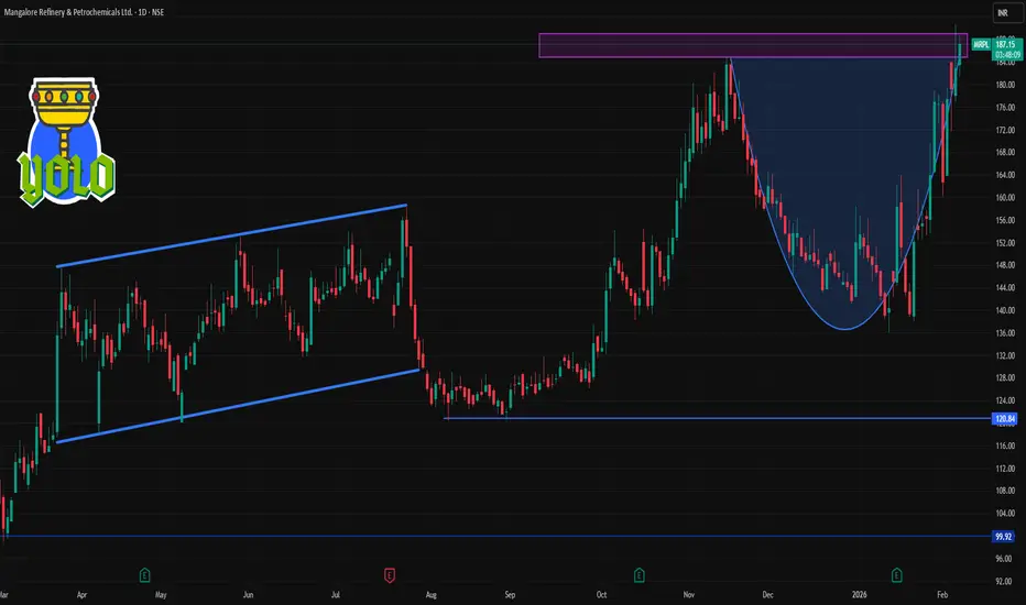
MRPL 1 Day Time Frame 📊 Latest Price Context (daily):
• The stock has recently been trading around ₹184–188 on NSE/BSE on the current session.
⭐ Daily Pivot Levels (Classic / Standard)
(used by many traders for intraday bias)
Level ₹ Price
R3 (Upper resistance) ~197.27
R2 ~190.63
R1 (Immediate resistance) ~184.97
Pivot Point (PP) ~178.33
S1 (Immediate support) ~172.67
S2 ~166.03
S3 ~160.37
👉 Interpretation:
Above Pivot (178–180) → bullish bias intraday.
Below Pivot → bearish / correction bias.
Resistance clusters near 185–191, with strong upper resistance around 197.
Immediate supports around 173 and 166 zones.
🔁 Alternate Daily Levels (Trendlyne)
(corroborated by another pivot source)
R1: ~₹185
R2: ~₹191
S1: ~₹172
S2: ~₹171 / ~₹168 (minor)
👉 Very similar structure: range ~172–185 for the day, with next larger moves beyond these points.
📌 Short Summary for 1-Day Trading Bias
Bullish if:
MRPL holds above daily pivot ~178–180
Break / close above ~185 could trigger further upside toward ~190–197
Bearish if:
Break below ~172 support
Next support zones: ~166 → ~160 area
Part 2 Technical Analysis VS. Institutional Option TradingStrike Price
The fixed price at which you can buy/sell.
Example: Nifty 22,000 CE = option to buy Nifty at 22,000.
Premium
The price of the option contract.
Paid by the buyer, received by the seller (writer).

INDUSTOWER 1 Day Time Frame 📌 1-Day Time Frame Levels (Daily Support & Resistance)
(These are typical pivot / intraday key levels traders watch)
Central Pivot (Pivot Point / CPR): ~ ₹421–₹422
Immediate Resistance Levels:
• R1: ~ ₹425–₹430
• R2: ~ ₹431–₹437
• R3: ~ ₹443–₹447
Immediate Support Levels:
• S1: ~ ₹415–₹417
• S2: ~ ₹411–₹414
• S3: ~ ₹405–₹408
(These pivot levels help gauge intraday bullish/bearish bias)
🧠 How to Interpret These Daily Levels
✔ If price stays above the pivot (~₹421–₹422) → bias is bullish for the day.
✔ A breakout above ₹430–₹437 may target higher resistances (~₹443+).
✔ A break below ~₹415–₹414 support could open the path toward lower supports (~₹405).
✔ Price oscillating between ~₹414 and ~₹422 is likely range-bound / choppy.
📊 Alternate/Additional Daily Levels (Trend Zones)
Some recent pivot-based grids suggest:
• First resistance: ~ ₹433–₹438
• Second resistance: ~ ₹438–₹443+
• Support zones: ~ ₹422–₹417, then ₹412–₹405 below that.

RECLTD 1 Day Time Frame 📍 Current Price (approx): ₹380–₹382 on NSE today (traded between ₹369.5–₹386.5 earlier) — price varies by source but this is the latest range.
📈 Daily Technical Levels (1-Day Timeframe)
🔁 Pivot & Reference
Daily Pivot Point: ~ ₹378–₹382 — central reference for bullish/bearish bias.
🟢 Resistance Levels
These are price zones where upside may face selling pressure:
R1: ~ ₹383–₹386 — first key resistance.
R2: ~ ₹390–₹397 — next resistance zone.
R3: ~ ₹400–₹402+ — extended resistance if trend continues up.
🔴 Support Levels
These are levels where price may find buying support in a pullback:
S1: ~ ₹378–₹379 — immediate support near pivot area.
S2: ~ ₹374–₹375 — deeper support zone.
S3: ~ ₹367–₹368 — secondary lower support.
📊 Short-Term Bias Interpretation (Daily View)
Bullish if:
✔ Price stays above the pivot (~₹378–₹382) and clears R1 (~₹383–₹386) — next upside towards R2 (~₹390+).
Neutral / Consolidating if:
↔ Price moves sideways around pivot without breakout — chop likely.
Bearish if:
✔ Price breaks below S1 (~₹378) — could test S2 (~₹374) and S3 (~₹367–₹368).
📌 Quick Summary (Daily)
Level Price (Approx)
Pivot (PP) ~₹378–₹382
Resistance 1 (R1) ~₹383–₹386
Resistance 2 (R2) ~₹390–₹397
Resistance 3 (R3) ~₹400–₹402+
Support 1 (S1) ~₹378–₹379
Support 2 (S2) ~₹374–₹375
Support 3 (S3) ~₹367–₹368
Note: These are daily pivot-based levels for short-term view. Price action can differ intraday due to volatility.

DAILY FOREX SCAN Session – 25 05 02 26Scanning multiple forex pairs to filter high-quality trade setups. No trades are forced—only structure-based opportunities.
Note: There may be a delay in this video due to upload processing time.
Disclaimer: FX trading involves high leverage and substantial risk, and losses can exceed your initial investment. This content is for educational purposes only and should not be considered financial advice. Trade at your own risk.

Automotive AxleDate 05.02.2026
Automotive Axle
Timeframe : Weekly Chart
Automotive Axles Ltd is positioned to benefit from recently announced India-EU Free Trade Agreement (FTA) as market expansion & specialised edge in Drive Axles, Front Steer Axles, Off-highway Axles, Non-Drive Axles, Drum & Disc Brake Suspension catering to the needs of Trucks and Buses Manufacturers in segments like light, medium, and heavy commercial vehicles, military and off-highway vehicles.It also provides aftermarket solutions to its customers
About
Established in 1981 as a JV of Kalyani Group (35.5% ownership) and Meritor Inc, USA (35.5% ownership)
Key Clients
Mahindra, Ashok Leyland, Tata, CAT, Bharat Forge, SML, VE commercial vehicles etc.
Product-wise Revenue
(1) Rear Drive Axles: 57%
(2) Brakes: 22%
(3) Other Parts: 21%
Valuations
(1) Market Cap ₹ 2,965 Cr
(2) Stock Pe 18
(3) Roce 22.3%
(4) Roe 16.6%
(5) Book Value 3X
(6) Opm 11%
(7) Promoter 71%
(8) Profit Growth (TTM) 7%
(9) EV/Ebita 11.49
(11) PEG 0.65
Regards,
Ankur

Part 1 Technical Analysis VS. Institutional Option Trading What Are Options?
Options are contracts that give you the right but not the obligation to buy or sell an asset at a fixed price before a certain date.
They are derivative instruments — their value comes from the underlying asset (index, stock, commodity, currency).
Options are mostly used for hedging, speculation, and income generation.
Two Types of Options
Call Option (CE): Right to buy at a chosen price.
Put Option (PE): Right to sell at a chosen price.

GMDC 1 Day Time Frame from NSE data:
📊 Daily Pivot & Key Levels (1D Timeframe)
📌 Daily Pivot Point (PP): ₹606.73 – This is the central bias level. Above this suggests short-term bullish control; below may signal weakness.
💥 Resistance Levels (Upside)
R1: ₹627.46 – first major resistance above the pivot
R2: ₹640.38 – medium-term barrier
R3: ₹661.11 – stronger supply zone / higher target
🛡️ Support Levels (Downside)
S1: ₹593.81 – immediate daily support
S2: ₹573.08 – deeper pullback level
S3: ₹560.16 – stronger lower support area
✔ How to use these levels (Daily view):
📈 Bullish conditions:
If price sustains above Pivot (₹606.73) → bias turns bullish
Stronger breakout confirmation if price closes above R1/R2 with volume
📉 Bearish conditions:
If price breaks below S1 (₹593.81) → watch for next supports (S2/S3)
Failure at resistance zones can lead to pullbacks
💡 Summary Daily Chart Levels (1D)
Level Price (Approx)
R3 661
R2 640
R1 627
Pivot 606
S1 594
S2 573
S3 560
(Levels rounded for clarity)

IFCI 1 Day Time Frame 📊 Current Live Price (Approx)
• IFCI trading around ₹57-₹60 range today on NSE/BSE (price fluctuates intraday).
✅ 1-Day Pivot & Key Levels
These are calculated based on recent price action and used by traders for intraday/short-term decisions:
Daily Pivot (PP): ~ ₹56.33 – ₹56.93
Resistance Levels:
R1: ~ ₹57.86 – ₹58.45
R2: ~ ₹59.06 – ₹60.14
R3: ~ ₹60.98 – ₹61.55
Support Levels:
S1: ~ ₹54.61 – ₹55.80
S2: ~ ₹53.08 – ₹53.68
S3: ~ ₹49.83 – ₹49.83 (deeper support)
📌 Ranges vary slightly by pivot calculation method (Classic, Fibonacci, Camarilla), but the zones above reflect current intraday technical consensus.
📌 How Traders Use These Levels (Daily View)
Bullish view:
• A sustained break above R1/R2 (~₹58-₹60) suggests strength and possible move toward R3 (~₹61+).
• Above pivot (~₹56-₹57) indicates bullish bias for the day.
Bearish view:
• A break below S1 (~₹54.6-₹55) can lead toward S2 (~₹53) and lower support.
• Below pivot signals downside pressure first.
🧠 Important Notes
• These levels are intraday technical references, not fundamental buy/sell calls.
• Markets and prices change minute-to-minute — use live quotes from your broker or trading platform.
• Combine pivot zones with volume, candlestick patterns, and trend indicators for better signals.

XAUUSD 15M – Bearish Structure Holding, Liquidity in PlayGold continues to respect a bearish market structure on the 15-minute timeframe after a clear rejection from the 50 & 200 EMA cluster, confirming a short-term trend shift in favor of sellers. The breakdown below the 0.618–0.786 Fibonacci retracement zone highlights strong distribution, with rallies being sold rather than accepted.
The MA Ribbon has fully turned bearish, acting as dynamic resistance around 4,930–4,950. As long as price remains below this supply zone, upside attempts are corrective in nature. No valid bullish displacement or reclaim has been established so far.
Momentum supports the downside: RSI (14) near 37 reflects sustained bearish strength without oversold exhaustion, leaving room for continuation. Prior RSI divergence has already played out, reinforcing the validity of the current move.
From a liquidity perspective, price is naturally drawn toward sell-side liquidity resting at 4,880 → 4,850, with an extended objective near 4,792, aligning with prior demand and measured move projections. Acceptance below these levels would likely open the door for further imbalance fills.
Directional Bias: Bearish below 4,950
Downside Liquidity Targets: 4,880 → 4,850 → 4,792
Invalidation: Strong reclaim and sustained acceptance above 4,980
⚠️ This is a liquidity-driven market — wait for confirmation, not anticipation.

Open Interest (OI) Analysis for Futures & Options TradersOpen Interest Analysis for Futures & Options Traders
Open Interest (OI) is one of the most powerful yet misunderstood tools in the derivatives market. While price and volume tell traders what is happening, open interest helps explain why it is happening and who is likely behind the move. For futures and options traders, OI analysis provides insight into market participation, strength of trends, potential reversals, and the behavior of smart money.
This makes OI a critical component for traders dealing in index futures, stock futures, options, and commodity derivatives.
What Is Open Interest?
Open Interest refers to the total number of outstanding derivative contracts (futures or options) that are currently open and not settled. Each contract represents a buyer and a seller, and open interest increases when new positions are created and decreases when positions are closed or squared off.
Key points:
OI increases when a new buyer and new seller enter a trade
OI decreases when an existing buyer and seller close their positions
OI does not change when one trader transfers a position to another
Unlike volume, which resets daily, open interest is cumulative and reflects ongoing market commitment.
Difference Between Volume and Open Interest
Many traders confuse volume with open interest, but both serve different purposes.
Volume measures how many contracts were traded during a specific period
Open Interest measures how many contracts remain open at the end of that period
High volume with low OI suggests short-term activity or intraday trading, while rising OI indicates fresh positions and conviction. Professional traders always study price, volume, and OI together.
Why Open Interest Matters in Trading
Open interest is important because it:
Confirms trend strength
Identifies new money entering or leaving
Signals long buildup or short buildup
Helps detect trend exhaustion
Improves options strategy selection
Reveals support and resistance zones
In derivatives trading, price movement without OI confirmation is often unreliable.
Open Interest Analysis in Futures Trading
1. Price Up + OI Up → Long Buildup
This indicates new buyers are entering the market with confidence.
Bullish trend confirmation
Strong upward momentum
Suitable for trend-following strategies
Example: Index futures rally with rising OI often suggests institutional buying.
2. Price Down + OI Up → Short Buildup
This signals fresh short positions entering the market.
Bearish trend confirmation
Indicates strong selling pressure
Often seen during market breakdowns
Professional traders use this to stay aligned with downside momentum.
3. Price Up + OI Down → Short Covering
This move is driven by short sellers exiting their positions.
Temporary rally
Weak bullish structure
Often occurs near resistance or after panic selling
Such rallies may fade once short covering ends.
4. Price Down + OI Down → Long Unwinding
This shows existing long positions are being closed.
Bearish but often near support
Indicates trend exhaustion
Can lead to sideways movement or reversal
Smart traders watch for price stabilization after long unwinding.
Open Interest Analysis in Options Trading
Options OI provides even deeper insights because it shows market expectations across strike prices.
Call Option Open Interest
High Call OI indicates resistance
Call writing suggests bearish or neutral outlook
Call buying suggests bullish expectations
Put Option Open Interest
High Put OI indicates support
Put writing suggests bullish or neutral outlook
Put buying suggests bearish expectations
Put-Call Open Interest Ratio (PCR)
The PCR is calculated as:
PCR = Total Put OI / Total Call OI
Interpretation:
PCR < 0.7 → Overly bullish (market may correct)
PCR between 0.7–1.2 → Balanced market
PCR > 1.3 → Overly bearish (market may bounce)
PCR is best used as a sentiment indicator, not a standalone signal.
Open Interest Shifts and Strike Price Analysis
Options traders closely watch:
Change in OI rather than absolute OI
OI buildup near key strikes
Unwinding before major breakouts
If heavy Call OI at a strike starts unwinding while price approaches it, that resistance may break. Similarly, Put OI unwinding near support can signal downside risk.
Max Pain Theory and OI
Max Pain refers to the strike price where option buyers experience maximum loss and option sellers gain maximum profit at expiry. Markets often gravitate toward this level close to expiry due to option writers’ influence.
While not exact, Max Pain combined with OI analysis improves expiry-day precision trading.
Intraday OI Analysis
For intraday traders:
Rising price + rising OI = trend continuation
Sudden OI drop = position exit or profit booking
OI spikes near VWAP = institutional activity
Intraday OI analysis is especially effective in index futures and liquid stock futures.
Common Mistakes in Open Interest Analysis
Using OI without price confirmation
Ignoring OI change and focusing only on absolute values
Misinterpreting short covering as trend reversal
Trading OI without understanding market context
Over-relying on PCR alone
OI should always be part of a broader trading framework.
Combining OI with Technical Analysis
The best results come from combining OI with:
Support and resistance
Trendlines
Moving averages
Volume profile
Price action patterns
For example, a breakout above resistance with rising volume and rising OI is far more reliable than price alone.
Role of Open Interest for Smart Money Tracking
Institutional traders rarely chase price. They build positions gradually, which reflects in:
Rising OI at key price zones
Stable price with increasing OI (accumulation)
Sudden OI drop after sharp moves (distribution)
OI helps retail traders align with smart money behavior rather than emotional price moves.
Conclusion
Open Interest analysis is an essential skill for futures and options traders who want to understand market structure, sentiment, and positioning. While price shows the outcome of trading decisions, open interest reveals the commitment and conviction behind those decisions.
When used correctly, OI helps traders:
Confirm trends
Spot reversals early
Identify strong support and resistance
Improve risk management
Trade with institutional flow rather than against it
However, open interest should never be used in isolation. Its real power emerges when combined with price action, volume, and market context. Traders who master OI analysis gain a significant edge in navigating the complex world of futures and options trading.

Quarterly Results: High-Impact Trading Strategies1. Why Quarterly Results Matter So Much
Quarterly earnings influence markets because they:
Update real financial reality versus expectations
Reset valuation assumptions
Alter future growth outlooks
Trigger institutional rebalancing
Create liquidity surges and volatility expansion
Markets do not react to numbers alone. They react to the difference between expectations and reality, known as earnings surprise.
Key drivers of price reaction:
Revenue vs estimates
EPS vs estimates
Guidance upgrades/downgrades
Management commentary tone
Margin expansion or contraction
2. Pre-Earnings Trading Strategies
Pre-earnings trades aim to capture anticipation, positioning, and volatility buildup.
A. Earnings Run-Up Strategy
Many stocks trend upward before results due to:
Analyst upgrades
Institutional accumulation
Positive sector sentiment
Strategy logic
Buy strong stocks 2–4 weeks before earnings
Ride the momentum until just before results
Exit partially or fully before announcement
Best conditions
Strong relative strength vs index
Consistent higher highs and higher lows
Positive earnings history
Risk
Sudden negative leaks or macro shocks
B. Volatility Expansion Play
Implied volatility typically rises before earnings.
Approach
Trade breakout setups near key levels
Use tight stop losses
Target fast momentum moves
Technical focus
Compression patterns (triangle, flag, box range)
Rising volumes into earnings
Narrow daily ranges before expansion
C. Avoid Directional Bets Without Edge
Blindly buying or shorting before results is gambling. Pre-earnings trades should be momentum-based, not prediction-based.
3. Result-Day Trading Strategies (High Risk, High Reward)
Earnings day offers explosive opportunities—but also extreme risk.
A. Gap-Up Continuation Trade
When a stock gaps up strongly and holds above key levels:
Entry
After first 15–30 minutes
Above VWAP or opening range high
Confirmation
Strong volumes
Minimal selling pressure
Price acceptance above gap zone
Target
Measured move or intraday resistance
B. Gap-Up Failure (Fade Trade)
Not all positive results sustain.
Signs of failure
Price rejects opening highs
Heavy selling volume
Break below VWAP
Strategy
Short below VWAP with tight stop
Target gap fill or previous close
This works well when:
Valuations are stretched
Market sentiment is weak
Guidance disappoints despite good numbers
C. Gap-Down Reversal (Dead Cat Bounce or True Reversal)
Large gap-downs can lead to:
Panic selling
Forced institutional exits
Reversal signs
Long lower wicks
Volume climax
Stabilization near support
Only aggressive traders should attempt this strategy.
4. Post-Earnings Trading Strategies (Most Consistent)
Post-earnings trades are statistically safer because uncertainty is removed.
A. Earnings Momentum Continuation
Strong results often lead to multi-week trends.
Ideal setup
Breakout above long-term resistance
Rising volumes post earnings
Analyst upgrades after results
Holding period
Days to weeks
Tools
Moving averages
Trend channels
Trailing stop losses
B. Post-Earnings Drift Strategy
Markets underreact initially and adjust over time.
Characteristics
Gradual trend continuation
Pullbacks bought aggressively
Strong relative strength
This is one of the most reliable earnings-based strategies.
C. Earnings Breakdown Short Trade
Negative earnings surprises can cause:
Structural trend breakdowns
Long-term distribution
Entry
Breakdown below support after results
Failed pullback retests
Target
Next major support zones
Best for:
High-debt companies
Weak cash flows
Deteriorating guidance
5. Sector and Index Influence
Earnings reactions depend heavily on:
Sector sentiment
Index trend (NIFTY, SENSEX, NASDAQ, S&P 500)
Example
Strong results in a weak market may still fail
Moderate results in a bullish sector may outperform
Always align earnings trades with:
Sector momentum
Broader market structure
6. Position Sizing and Risk Management
Quarterly results can move stocks 5–25% overnight.
Key risk rules:
Never risk more than 1–2% of capital per earnings trade
Reduce position size compared to normal trades
Avoid overexposure to multiple earnings trades at once
Respect gap risk—stop losses don’t work overnight
7. Common Mistakes Traders Make
Trading earnings without a plan
Ignoring guidance and commentary
Overtrading on result day
Holding losing trades hoping for reversal
Confusing good numbers with good price action
Remember: Price reaction > numbers
8. Professional Trader’s Earnings Checklist
Before every earnings trade:
Is the stock in a trend?
What is the market expecting?
How has the stock reacted to past earnings?
Where are key support/resistance levels?
What is my predefined risk?
If these answers aren’t clear, skip the trade.
9. Long-Term Perspective
Earnings trading is not about predicting results—it’s about reacting faster and smarter than the crowd. Professionals wait for confirmation, manage risk ruthlessly, and trade only high-quality setups.
The best traders treat earnings as:
Volatility opportunities
Trend accelerators
Risk events to be respected
Conclusion
Quarterly results are among the highest-impact events in financial markets, capable of reshaping trends in minutes and defining direction for months. High-impact earnings trading requires discipline, preparation, technical awareness, and emotional control.
Traders who focus on price behavior, volume confirmation, and post-earnings trends—rather than predictions—consistently outperform those who gamble on numbers alone.
