Understanding the Master Candle ConceptOption trading is one of the most exciting and flexible segments of the financial markets. It allows traders to profit not only when prices rise, but also when they fall — and even when they stay relatively stable. In simple terms, an option is a financial contract that gives the buyer the right, but not the obligation, to buy or sell an underlying asset at a predetermined price within a specified period. In India, options are primarily traded on stock indices (like NIFTY 50 or BANK NIFTY) and individual stocks on exchanges like the NSE (National Stock Exchange) and BSE (Bombay Stock Exchange).
Option Trading in India – Regulations
Option trading in India is regulated by the Securities and Exchange Board of India (SEBI).
Contracts are standardized and traded through exchanges like NSE and BSE.
All participants must trade through SEBI-registered brokers, and margins are monitored daily to control risk.
Trend Line Break

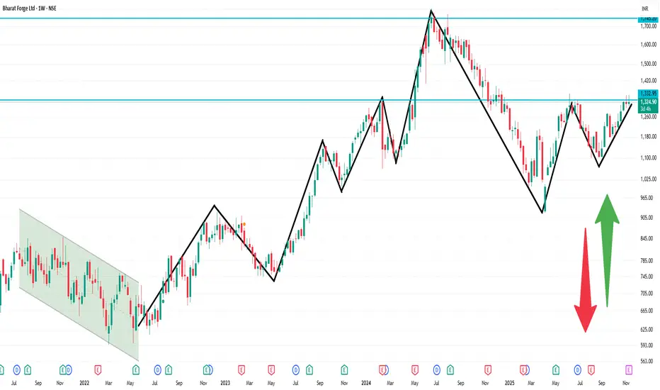
Bharat Forge (D): Strongly Bullish, Multi-Resistance BreakoutThis is a high-conviction breakout event. The stock has decisively broken out of a 17-month corrective pattern, shattering two major resistance levels simultaneously. This move is supported by a powerful confluence of bullish indicators across all timeframes and is underpinned by strong fundamental results.
📈 1. The Long-Term Context
- The Correction: After hitting its All-Time High (ATH) in June 2024 , the stock entered a 10-month corrective downtrend.
- The Reversal: This trend reversed in April 2025 , and the stock began a new recovery.
- The Consolidation: This recovery was capped by two distinct resistance levels, forcing the stock into a consolidation phase where, volume was drying up (a sign of accumulation).
🚀 2. The Decisive Breakout (Today's Action)
Today, the stock broke this stalemate with explosive force:
- The Surge: A powerful +5.55% rally on high-conviction volume of 4.81 Million shares.
- The Dual Breakout: This move shattered both key resistance levels at once:
1. The long-term angular resistance (from the June 2024 ATH).
2. The short-term horizontal resistance (from June 2025, at the ₹1,362 level).
- The Catalyst: This technical breakout is supported by strong Q2 earnings, which act as a fundamental driver, giving the move a higher probability of success.
📊 3. Confluence of Bullish Indicators
This breakout is not isolated. It is confirmed by a rare "trifecta" of bullish signals on Daily, Weekly, and Monthly timeframes:
- RSI: The Relative Strength Index is rising on all three timeframes .
- EMAs: The short-term Exponential Moving Averages are in a "PCO" (Price Crossover) state on all three timeframes .
- SMAs: A recent SMA Golden Cross (50-day crossing 200-day) is active, confirming the new long-term uptrend.
🎯 4. Future Scenarios & Key Levels to Watch
This breakout provides a very clear road map based on identified levels:
🐂 The Bullish Case (Momentum Continues)
- Trigger: If the current momentum is sustained, the stock is in a new uptrend.
- Target 1 (Short-Term): ₹1,525
- Target 2 (Medium-Term): ₹1,625
🐻 The Pullback Scenarios
- Scenario A (Healthy Re-test): The momentum pauses, and the stock pulls back to test the "resistance-turned-support" level at ₹1,362 . A bounce from here would be a textbook confirmation and a secondary buying opportunity.
- Scenario B (Breakout Failure): If the breakout is a "fakeout," the stock will fail to hold ₹1,362 and will likely fall to the next major support level at ₹1,305 .

BUY TODAY SELL TOMORROW for 5%DON’T HAVE TIME TO MANAGE YOUR TRADES?
- Take BTST trades at 3:25 pm every day
- Try to exit by taking 4-7% profit of each trade
- SL can also be maintained as closing below the low of the breakout candle
Now, why do I prefer BTST over swing trades? The primary reason is that I have observed that 90% of the stocks give most of the movement in just 1-2 days and the rest of the time they either consolidate or fall
Trendline Breakout in POLYMED
BUY TODAY SELL TOMORROW for 5%

BUY TODAY SELL TOMORROW for 5%DON’T HAVE TIME TO MANAGE YOUR TRADES?
- Take BTST trades at 3:25 pm every day
- Try to exit by taking 4-7% profit of each trade
- SL can also be maintained as closing below the low of the breakout candle
Now, why do I prefer BTST over swing trades? The primary reason is that I have observed that 90% of the stocks give most of the movement in just 1-2 days and the rest of the time they either consolidate or fall
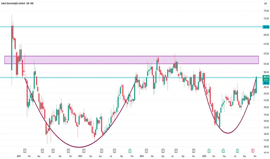
Trendline Breakout in LATENTVIEW
BUY TODAY SELL TOMORROW for 5%

BUY TODAY SELL TOMORROW for 5%DON’T HAVE TIME TO MANAGE YOUR TRADES?
- Take BTST trades at 3:25 pm every day
- Try to exit by taking 4-7% profit of each trade
- SL can also be maintained as closing below the low of the breakout candle
Now, why do I prefer BTST over swing trades? The primary reason is that I have observed that 90% of the stocks give most of the movement in just 1-2 days and the rest of the time they either consolidate or fall
Trendline Breakout in LUMAXTECH
BUY TODAY SELL TOMORROW for 5%

How to Use Candlestick Patterns in TradingA candlestick represents price movement for a given time frame.
It shows:
Open price – where the candle started
Close price – where the candle ended
High price – the top point (shadow or wick)
Low price – the bottom point (shadow or wick)
👉 If the close price > open price, it’s a bullish candle (often green or white).
👉 If the close price < open price, it’s a bearish candle (often red or black).

Understanding The Premium Chart Patterns 1. Hedging: To protect against losses in existing positions.
Example: If you own Nifty stocks but fear a market fall, buying a put option acts as insurance.
2. Speculation: To profit from expected price movements with limited risk.
Example: Buying a call if you expect prices to rise.
3. Income Generation: Selling (writing) options to earn a premium — the price paid by the buyer of the option.

Advanced Option Trading StrategiesHedging and Portfolio Protection Strategies
Options are not just for speculation; they are powerful tools for hedging existing stock portfolios. Hedging means protecting against potential losses due to adverse price moves.
Popular Hedging Techniques:
Protective Put: Buy a put option against long stock holdings to limit downside.
Collar Strategy: Hold stock, sell a call, and buy a put — ideal when you expect limited movement.
Index Options for Portfolio Hedge: Traders holding multiple stocks often hedge using Nifty or Bank Nifty puts instead of individual stock options.

Part 12 Trading Master ClassImportance of Time Decay (Theta)
Another vital concept in options trading is Theta, which measures how much the value of an option decreases as it approaches expiry — this is called time decay.
Buyers of options lose value daily because the time value erodes.
Sellers (writers) benefit from time decay as they collect premium that melts away if the market remains range-bound.

Part 11 Trading Master ClassTaxation and Regulations in India
In India:
Profits from options trading are treated as business income.
Traders must file under F&O income while filing Income Tax.
Options trading is regulated by SEBI and executed through NSE/BSE.
Always ensure you trade only through authorized brokers and maintain proper records for compliance.

Part 9 Trading Master ClassChoosing the Right Strategy
Selecting the right options strategy depends on three factors:
Market Outlook:
Bullish → Long Call, Bull Call Spread, Short Put
Bearish → Long Put, Bear Put Spread, Covered Call
Neutral → Iron Condor, Butterfly, Short Straddle
Volatility:
High volatility → Buy options (Straddle, Strangle)
Low volatility → Sell options (Condor, Credit spreads)
Risk Appetite:
Low-risk → Spreads
Medium-risk → Covered/Protective positions
High-risk → Naked calls/puts

Part 10 Trade Like InstitutionsAdvanced Option Strategies
a) Butterfly Spread
Market View: Very Neutral (Expecting Minimal Movement)
Action: Buy 1 lower strike call + Sell 2 middle strike calls + Buy 1 higher strike call.
It profits if the market remains near the middle strike.
Risk: Limited.
Reward: Limited but high probability of success.
b) Calendar Spread
Market View: Expecting Low Short-Term Volatility but High Long-Term Movement
Action: Sell near-month option + Buy next-month option of same strike.
Used by professional traders to take advantage of time decay differences between expiries.

Part 8 Trading master Class Types of Option Trading Strategies
Options strategies are broadly divided into single-leg and multi-leg strategies.
Single-leg strategies: Involve buying or selling one option.
Multi-leg strategies: Combine two or more options (calls and puts) to create structured trades for specific market conditions.
Let’s discuss each category in detail.

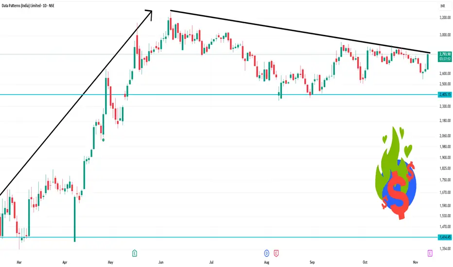
DATAPATTNS 1 Day Time Frame 📋 Key Levels
Accumulated-volume support: ≈ ₹2,576.90.
Fibonacci-based support levels: ~ ₹2,514.67 & ~ ₹2,545.65.
Short-term support (MarketScreener): ~ ₹2,541.40.
Resistance: ~ ₹2,806.80 (accumulated volume)
Short-term resistance (MarketScreener): ~ ₹2,842.
Moving averages:
20-day EMA ~ ₹2,750.69.
50-day EMA ~ ₹2,720.79.
LATENTVIEW 1 Week TIme Frame Latest closing price: ~ ₹ 428.60.
1-week return: approx +0.15%.
Key technical levels per one source:
Support 1: ~ ₹ 423
Support 2: ~ ₹ 410
Support 3: ~ ₹ 386
Pivot point: ~ ₹ 447
Resistance 1: ~ ₹ 460
Resistance 2: ~ ₹ 484
Resistance 3: ~ ₹ 498
BHARATFORG 1 Week TIme Frame 🔍 Current Snapshot
Latest price approx ₹1,320 (rounded) as per recent quotes.
52-week range: ~₹919 (low) to ~₹1,482 (high).
Valuation: P/E ~60x and P/B ~6–7x.
Key sectors: auto-ancillaries, defence & aerospace.
📉 Key Technical Levels (Short-Term, ~1 Week)
Based on support/resistance and recent trading behaviour, here are levels to watch:
Support: around ₹1,250-1,260. If the price drops and finds buying interest, this is a potential floor zone.
Resistance: near ₹1,350-1,370. If momentum builds, breaking above this could open for further short-term upside.
Watch for range-bound behaviour: If neither major catalyst nor breakdown happens, expect the stock to oscillate between ~₹1,260 and ~₹1,350 in the coming week.
WELSPUNLIV 1 Day Time Frame📌 Current price
Last seen around ₹129–130.
The 52-week high is ~ ₹180.70 and the 52-week low ~ ₹104.80.
📊 Key 1-day support & resistance / pivots
From recent technical data:
Daily pivot (central) around ~ ₹131.08.
Support levels (approx):
S1 ~ ₹129.07
S2 ~ ₹125.88
Resistance levels (approx):
R1 ~ ₹134.27
R2 ~ ₹136.28

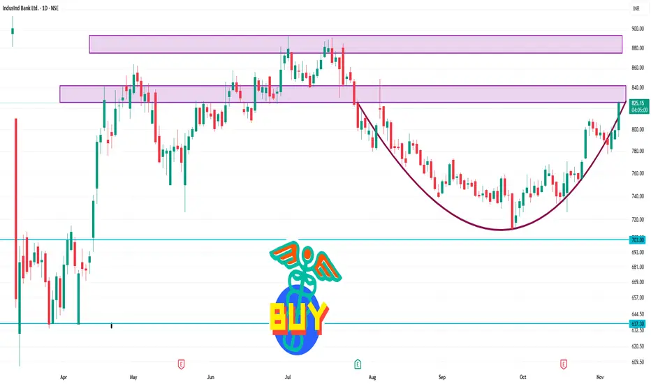
INDUSINDBK 1 Day Time Frame Level 🔍 Current snapshot
Latest live price: ~ ₹825.00.
Today’s approximate range: Low ~ ₹792.80, High ~ ₹826.00.
52-week range: Low ~ ₹606.00, High ~ ₹1,086.55.
📈 Key support & resistance levels
Support zone: ~ ₹790-₹800 — because price has held above ~₹792 today and that region shows earlier low of day.
Immediate resistance: ~ ₹825-₹830 — since the current price is around ₹825; breaking above that may open up.
Stronger resistance: ~ ₹850+ — if momentum builds, aim toward next psychological level.
Deeper support: if price falls below ₹790, next meaningful support could be ~ ₹760-₹770 (not precisely calculated but logical given range).
FINCABLES 1 Day View 📌 Current Price Snapshot
Latest close around ₹ 785.40.
Day’s trading range: roughly ₹ 784 – ₹ 793.95.
52-week range: low ~ ₹ 779.80, high ~ ₹ 1,342.75.
🧭 Key Technical Levels to Watch
Support zone: ~ ₹ 780–790 — price is near its 52-week low and this band may act as immediate support.
Resistance zone: ~ ₹ 800–810 — recent highs in this area, so a breakout above this could be meaningful.
If support breaks: A decisive break below ~₹ 780 could open downside risk; monitor volume.
If resistance breaks: A strong move above ~₹ 810 with volume could target next levels (₹ 820-850+), though those are less “immediate” on one-day timeframe.
✅ What to monitor today
Closing price relative to the above levels (did it hold above support or test resistance?).
Volume — whether any breakout/breakdown is backed by increased activity.
Price reaction around the ₹ 780-790 support band: a bounce could indicate strength; a failure might signal weakness.

Technical Analysis and Chart PatternsIntroduction
Technical analysis is a cornerstone of modern trading and investing. It involves studying price charts and market data to forecast future price movements. Unlike fundamental analysis, which focuses on financial statements, earnings, and economic indicators, technical analysis revolves around price action, volume, and market psychology. It assumes that all relevant information is already reflected in the price, and history tends to repeat itself through recognizable chart patterns and trends.
Core Principles of Technical Analysis
Technical analysis operates on three main principles:
Price Discounts Everything:
All known information—economic data, earnings, market sentiment, or political events—is already factored into the stock price. Therefore, analyzing price action alone can reveal the collective behavior of market participants.
Price Moves in Trends:
Markets rarely move randomly. Prices tend to move in identifiable trends—upward, downward, or sideways. Recognizing these trends early allows traders to position themselves advantageously.
History Repeats Itself:
Human psychology drives markets—fear, greed, hope, and panic repeat across generations. Therefore, patterns formed in the past tend to recur, providing clues about future price action.
Types of Technical Charts
Before identifying patterns, one must understand chart types used in technical analysis:
Line Chart:
It connects closing prices over a specific period, providing a simple view of the trend.
Bar Chart:
Each bar represents the open, high, low, and close (OHLC) for a given period. It gives more insight than a line chart.
Candlestick Chart:
The most popular chart among traders, candlesticks visually show market psychology. A bullish candle (close > open) is often green or white, while a bearish candle (close < open) is red or black.
Candlestick formations help identify reversals and continuations in price.
Trend Analysis
A trend is the general direction of price movement. It can be classified as:
Uptrend: Series of higher highs and higher lows.
Downtrend: Series of lower highs and lower lows.
Sideways/Range: Prices oscillate between support and resistance.
Traders use trendlines and channels to visualize and trade along the trend. The saying “Trend is your friend” highlights the importance of trading with the prevailing direction rather than against it.
Key Tools in Technical Analysis
Support and Resistance Levels:
Support: A price level where buying pressure prevents further decline.
Resistance: A level where selling pressure halts price advances.
When a resistance is broken, it can turn into new support and vice versa.
Moving Averages:
They smooth out price data to identify trend direction.
Simple Moving Average (SMA) – average of closing prices over a period.
Exponential Moving Average (EMA) – gives more weight to recent prices.
Common crossovers like the Golden Cross (short-term MA crosses above long-term MA) and Death Cross (short-term MA crosses below long-term MA) indicate trend reversals.
Volume Analysis:
Volume measures market participation. Increasing volume confirms the strength of a trend, while declining volume may signal weakening momentum.
Indicators and Oscillators:
Tools like Relative Strength Index (RSI), Moving Average Convergence Divergence (MACD), Bollinger Bands, and Stochastic Oscillator help identify overbought/oversold conditions, momentum shifts, and trend confirmation.
Chart Patterns in Technical Analysis
Chart patterns are visual formations created by price movements. They represent the psychological struggle between buyers and sellers and help traders predict potential outcomes.
Patterns are generally divided into reversal patterns and continuation patterns.
1. Reversal Patterns
These indicate that a current trend is likely to change direction.
a. Head and Shoulders
One of the most reliable reversal patterns.
Appears at the end of an uptrend.
Consists of three peaks: a higher middle peak (head) between two smaller ones (shoulders).
Neckline break confirms a bearish reversal.
Inverse Head and Shoulders appears at the bottom of a downtrend and signals a bullish reversal.
b. Double Top and Double Bottom
Double Top: Price hits a resistance twice, forming an “M” shape, signaling a bearish reversal.
Double Bottom: Price touches support twice, forming a “W” shape, indicating a bullish reversal.
c. Triple Top and Triple Bottom
Similar to double patterns but with three peaks or troughs. They confirm stronger reversals after multiple failed attempts to break support/resistance.
d. Rounding Bottom (Saucer Bottom)
Indicates a gradual shift from bearish to bullish sentiment over time. Common in long-term trend reversals.
e. Falling and Rising Wedges
Falling Wedge: Occurs during a downtrend and signals a bullish reversal.
Rising Wedge: Forms during an uptrend and signals a bearish reversal.
The breakout direction typically opposes the wedge slope.
2. Continuation Patterns
These suggest that the existing trend will continue after a brief pause or consolidation.
a. Triangles
Ascending Triangle: Horizontal resistance with rising support. Usually bullish.
Descending Triangle: Horizontal support with falling resistance. Usually bearish.
Symmetrical Triangle: Converging trendlines; breakout can occur in either direction.
b. Flags and Pennants
Flags: Small rectangular consolidations that form after a sharp move (flagpole). Breakout in the same direction resumes the prior trend.
Pennants: Similar to flags but shaped like small symmetrical triangles.
c. Rectangles (Price Channels)
When price oscillates between parallel support and resistance lines, it indicates accumulation or distribution. A breakout determines the next direction.
d. Cup and Handle
Looks like a tea cup: a rounded “cup” followed by a small “handle” consolidation. A breakout above the handle signals bullish continuation.
Candlestick Patterns
In addition to chart patterns, candlestick patterns offer short-term trading signals:
Bullish Engulfing: Large bullish candle engulfs the previous bearish candle—signals buying momentum.
Bearish Engulfing: Large bearish candle engulfs the previous bullish one—signals selling pressure.
Doji: Open and close prices are nearly equal, indicating indecision.
Hammer & Inverted Hammer: Found at bottoms, indicating potential reversals.
Shooting Star: Appears at tops, suggesting bearish reversal.
Combining Patterns with Indicators
Professional traders often combine chart patterns with technical indicators for confirmation.
Example:
A head and shoulders pattern confirmed by falling RSI strengthens the bearish outlook.
A cup and handle confirmed by rising volume adds validity to a bullish move.
This multi-factor approach reduces false signals and increases accuracy.
Advantages of Technical Analysis
Quick Decision-Making: Real-time charts provide instant trading opportunities.
Universal Application: Works across stocks, forex, commodities, and crypto.
Captures Market Psychology: Reflects fear and greed through patterns.
Supports Short-Term Trading: Ideal for day traders and swing traders.
Limitations of Technical Analysis
Subjectivity: Two traders may interpret the same chart differently.
False Breakouts: Patterns may fail, especially in volatile markets.
Lagging Indicators: Some tools like moving averages react after price changes.
No Fundamental Insight: It ignores earnings, news, and macroeconomic data.
Conclusion
Technical analysis is both an art and a science. By studying chart patterns, trends, and indicators, traders can anticipate potential price moves with greater confidence. However, success in technical analysis demands discipline, patience, and risk management. Patterns don’t guarantee results; they only increase probabilities. Combining chart patterns with volume analysis, market context, and proper stop-loss strategies creates a strong foundation for consistent profitability.
Ultimately, mastering technical analysis means understanding how market psychology shapes price movements—and using that knowledge to stay one step ahead of the crowd.
Private vs Public Banks in the Indian Market1. Ownership and Management Structure
The fundamental difference between public and private banks lies in ownership.
Public Sector Banks (PSBs) are majority-owned by the Government of India, which holds more than 50% of their equity. The government plays a key role in appointing top executives and formulating policy directions. Examples include State Bank of India (SBI), Punjab National Bank (PNB), Bank of Baroda (BoB), and Canara Bank.
Private Sector Banks (PVBs), on the other hand, are owned and managed by private entities or individuals, with the government having little or no control. The management is typically professional, and boards are accountable to private shareholders. Major private banks include HDFC Bank, ICICI Bank, Axis Bank, Kotak Mahindra Bank, and IndusInd Bank.
This difference in ownership affects how both types of banks operate, their decision-making processes, and their responsiveness to market conditions.
2. Historical Background
Public sector banks form the backbone of India’s traditional banking system. They gained prominence after bank nationalization in 1969 and 1980, which brought 20 major banks under government control. The aim was to ensure that banking services reached rural and underbanked areas, supporting agriculture, small industries, and social development.
Private banks, however, emerged in two waves:
The first phase included old private banks such as Karur Vysya Bank, South Indian Bank, and Federal Bank, which were regional and limited in scale.
The second phase, or the “new generation” private banks, began after the economic liberalization of 1991, when the Reserve Bank of India (RBI) allowed new private players to enter. Banks like HDFC Bank, ICICI Bank, and Axis Bank brought innovation, technology, and competition to the market.
3. Operational Efficiency and Technology
Private sector banks are widely recognized for their efficiency and technological advancement. They were pioneers in introducing digital banking, internet and mobile apps, ATMs, 24/7 customer service, and AI-based financial solutions. Their focus on automation and quick service appeals especially to urban customers.
Public banks, though initially slower to adopt technology, have made significant progress in recent years. Initiatives like YONO by SBI, Bank of Baroda’s digital transformation, and PSB Alliance have modernized public banking. However, public banks still face challenges due to their vast legacy systems and bureaucratic procedures.
4. Customer Service and Experience
Private banks are often perceived as offering superior customer service, with faster processing times, personalized products, and proactive relationship management. Their staff is trained to focus on efficiency and customer satisfaction.
Public banks, however, have traditionally been known for longer processing times and formal procedures. Yet, they provide an essential service to a larger section of society, especially in rural and semi-urban areas where private banks may not have strong penetration. PSBs are more committed to social welfare schemes such as Jan Dhan Yojana, Mudra loans, and agricultural credit programs.
5. Market Reach and Financial Inclusion
In terms of reach, public sector banks hold a dominant position. They have thousands of branches across rural India, ensuring that even remote populations have access to banking facilities. For instance, SBI alone accounts for more than 20% of India’s total banking network.
Private banks, conversely, focus primarily on urban and metropolitan regions where customers demand faster, technology-driven services. However, they are now expanding into Tier 2 and Tier 3 cities to capture a growing middle-class market.
6. Profitability and Performance
Private banks usually exhibit higher profitability, better asset quality, and more stable returns. Their operational flexibility, low non-performing asset (NPA) ratios, and efficiency in cost management contribute to superior financial performance. For instance, banks like HDFC and ICICI consistently report high return on assets (ROA) and return on equity (ROE).
Public banks, due to their social obligations and exposure to priority sectors, often face higher NPAs and lower profitability. Lending to agriculture, infrastructure, and small enterprises—though socially vital—sometimes leads to defaults. However, government support through recapitalization and mergers (like SBI with its associate banks) helps maintain their financial stability.
7. Lending Patterns and Risk Management
Public banks prioritize social and developmental objectives, lending to priority sectors such as agriculture, small industries, and low-income groups. They are also instrumental in implementing government schemes like PMEGP, Stand-Up India, and PM Kisan.
Private banks focus more on profitable segments such as retail loans, home loans, credit cards, and wealth management. They employ advanced risk assessment tools, AI-driven credit scoring, and market-based pricing, which help reduce bad loans and maintain better credit discipline.
8. Employment and Work Culture
Public sector banks provide job security, stable career paths, and government-linked benefits. They attract candidates through national-level exams conducted by IBPS or SBI. However, the work culture can be bureaucratic, hierarchical, and slower in decision-making.
Private banks offer performance-based incentives, faster promotions, and modern work environments, but job security is lower. They emphasize productivity, targets, and results, often leading to higher stress levels but better pay for top performers.
9. Regulatory Environment
Both public and private banks are regulated by the Reserve Bank of India (RBI) and governed by the Banking Regulation Act, 1949. However, PSBs are also accountable to the Ministry of Finance and the Parliament of India, which increases oversight but sometimes limits autonomy. Private banks enjoy greater independence in policy decisions but must adhere strictly to RBI norms.
10. Public Trust and Perception
Public banks enjoy a high level of trust among citizens, especially older generations and rural populations, because of government backing. Depositors believe their money is safe, even if the bank faces trouble, as the government is expected to intervene.
Private banks are viewed as modern, efficient, and customer-friendly, but public confidence fluctuates based on market performance. However, strong brands like HDFC Bank and ICICI Bank have built reputations rivaling public banks in reliability.
11. Future Trends and Outlook
The future of India’s banking sector lies in coexistence and collaboration between public and private players.
Public banks are likely to focus on financial inclusion, rural expansion, and implementation of government initiatives.
Private banks will continue to drive technological innovation, digital lending, and customer-centric growth.
Additionally, the rise of fintech companies, digital payments platforms (like Paytm and PhonePe), and neo-banks is pushing both sectors toward modernization and customer-focused strategies.
Government-led reforms such as bank mergers, recapitalization packages, and privatization plans indicate an evolving structure aimed at improving competitiveness and efficiency. As India’s economy grows, both public and private banks will play complementary roles in supporting national development and financial stability.
Conclusion
In summary, public sector banks represent the traditional, inclusive, and socially driven side of Indian banking, while private sector banks symbolize innovation, efficiency, and profit-oriented growth. Each has its strengths: public banks bring trust, accessibility, and social responsibility, while private banks bring technology, speed, and superior service quality.
The Indian market thrives on this balance — where government-backed institutions ensure inclusive development and private banks drive modernization and competition. Together, they form a robust dual system that continues to evolve, reflecting the dynamic needs of a rapidly developing economy.

Relative Strength Index (RSI) Indicator Secrets1. The Hidden Meaning Behind RSI Levels
Most traders use the 70/30 rule blindly. In reality, RSI levels are relative, not absolute. For instance:
In a strong uptrend, RSI can remain above 70 for a long period — this does not mean the market will immediately reverse. It often indicates strong bullish momentum.
In a downtrend, RSI can stay below 30 for an extended time — signaling strong bearish pressure, not necessarily an immediate bounce.
Secret Tip:
Adjust your RSI levels based on market conditions:
Bullish market: Use RSI zones of 40–80 (support around 40, resistance around 80).
Bearish market: Use RSI zones of 20–60 (resistance around 60, support around 20).
By doing this, you interpret RSI in the context of trend strength rather than treating it as an isolated signal.
2. RSI as a Trend Identifier
One of the most overlooked uses of RSI is trend confirmation. Traders often rely on moving averages or price patterns to identify trends, but RSI can do this more efficiently.
In uptrends, RSI tends to stay above 40 and frequently reach 70–80.
In downtrends, RSI remains below 60 and often hits 20–30.
Secret Insight:
If RSI repeatedly bounces from the 40–50 zone during a price pullback, it suggests that the uptrend is healthy. Conversely, if RSI fails to move above 60 during rallies, it signals weakness in the market.
This method helps traders stay with the trend longer, instead of prematurely exiting a position when RSI crosses traditional overbought or oversold levels.
3. RSI Divergence – The Ultimate Reversal Signal
RSI divergence is one of the strongest signals for trend reversal. It occurs when the price makes a new high or low that isn’t confirmed by the RSI.
Bullish Divergence: Price makes a lower low, but RSI makes a higher low — signaling potential upward reversal.
Bearish Divergence: Price makes a higher high, but RSI makes a lower high — indicating possible downward reversal.
Secret Tip:
For divergence to be effective, it must occur after a strong trend and be confirmed by volume or candlestick patterns (like Doji, hammer, or engulfing). Many traders lose money by trading every small divergence — patience is key.
Additionally, hidden divergence can predict trend continuation:
Hidden Bullish Divergence: RSI makes a lower low, but price makes a higher low → continuation of uptrend.
Hidden Bearish Divergence: RSI makes a higher high, but price makes a lower high → continuation of downtrend.
Combining regular and hidden divergences can give traders early entry signals and improve accuracy.
4. RSI Swing Rejections: The Secret Entry Technique
Welles Wilder’s original writings described an advanced RSI technique called “Swing Rejection”, which most traders overlook.
A bullish swing rejection occurs when:
RSI drops below 30 (oversold zone).
It rises above 30.
Pulls back but stays above 30.
Then breaks its previous high.
This pattern signals a strong bullish reversal — often before the price fully turns up.
A bearish swing rejection is the opposite:
RSI rises above 70.
Falls below 70.
Rebounds but fails to cross 70 again.
Then breaks its prior low — confirming weakness.
Secret Insight:
Swing rejections filter out false overbought/oversold signals and identify high-probability turning points in the market.
5. RSI with Multiple Time Frames
Professional traders rarely rely on a single RSI setting or timeframe. Instead, they confirm RSI signals across multiple timeframes.
For example:
If the daily RSI is oversold but the weekly RSI is still in a downtrend, the bounce may be short-lived.
When both daily and weekly RSI align in the same direction, it indicates a powerful trend reversal or continuation.
Secret Tip:
Use RSI(14) on higher timeframes (daily/weekly) for trend bias, and RSI(7) or RSI(9) on lower timeframes (hourly or 4-hour) for precise entries.
6. RSI and Moving Averages – A Smart Combination
Combining RSI with moving averages creates a more reliable trading system. For example:
Use a 50-period moving average to determine the trend direction.
Trade RSI signals only in the direction of the moving average.
Example:
If the price is above the 50-MA and RSI bounces from 40 → it’s a strong buy signal.
If the price is below the 50-MA and RSI drops from 60 → it’s a strong sell signal.
This combination filters out false signals and aligns trades with the dominant market trend.
7. RSI Range Shifts – The Professional Secret
A rarely discussed RSI secret is the concept of range shifts. In a strong uptrend, RSI tends to move between 40–80 instead of 30–70. In a strong downtrend, it shifts between 20–60. Recognizing this range shift early helps traders identify when the market transitions from sideways to trending behavior.
When RSI consistently fails to fall below 40 and pushes above 70, it confirms that bulls control the market. Conversely, when RSI struggles to rise above 60 and keeps hitting 30, bears dominate.
Spotting a range shift early can help you enter trends sooner and ride them longer.
8. Customizing RSI Periods for Different Assets
Most traders use the default 14-period RSI. However, adjusting the period can dramatically change its responsiveness:
Shorter RSI (5 or 7): More sensitive, gives early signals but more noise.
Longer RSI (20 or 30): Smoother, fewer false signals but more lag.
Secret Tip:
For volatile instruments like cryptocurrencies or small-cap stocks, use a shorter RSI (7–10).
For stable assets like large-cap stocks or indices, use longer RSI (14–21).
Customizing RSI settings according to volatility improves accuracy and reduces whipsaws.
9. Psychological Secrets of RSI
At its core, RSI reflects market psychology — the tug-of-war between buyers and sellers. When RSI rises above 70, it shows traders’ greed; when it falls below 30, it reveals fear. Understanding this helps you trade in the opposite direction of crowd emotions.
The best traders use RSI not just as a technical tool, but as a window into trader sentiment. Combining RSI readings with support/resistance zones or volume analysis offers a powerful edge.
10. Conclusion
The RSI indicator is far more than a simple overbought/oversold tool. Its true strength lies in understanding context, trend structure, divergence, and range behavior. By mastering RSI’s hidden secrets — such as swing rejections, range shifts, and multiple timeframe confirmations — traders can dramatically improve accuracy and timing.
When used intelligently, RSI reveals the rhythm of market momentum and helps traders ride trends, spot reversals, and stay on the right side of price action. Like all tools, it works best when combined with sound risk management, patience, and discipline — the true secrets behind profitable trading.
Artificial Intelligence (AI) has Revolutionized1. Introduction to AI in Trading
AI refers to the simulation of human intelligence through machines that can analyze data, learn from it, and make decisions with minimal human intervention. In trading, AI systems are designed to interpret large volumes of market data, recognize patterns, and execute trades based on pre-defined strategies or learned behaviors. These systems use techniques like machine learning, deep learning, and natural language processing (NLP) to improve performance over time.
Before the AI era, traders relied on intuition, experience, and manual technical analysis. They studied indicators like moving averages, RSI, and MACD, spending hours identifying potential entry and exit points. Today, AI can perform the same analysis within seconds — and with greater precision.
2. How AI Simplifies Trading
AI simplifies trading in multiple ways — from data analysis to strategy automation and risk management. Let’s break it down:
a. Data Processing Power
Markets generate massive amounts of data every second — stock prices, trading volumes, economic indicators, and news headlines. Humans can’t process such data in real time, but AI systems can. They analyze historical and live data simultaneously to identify trends, correlations, and anomalies.
For example, an AI algorithm can scan millions of trades across multiple exchanges to find a small arbitrage opportunity — something no human could do manually.
b. Automated Trading Systems
AI-powered bots can execute trades automatically based on predefined rules or predictive models. These algorithmic trading systems remove emotional decision-making — a common pitfall for human traders.
Once trained, an AI system can:
Identify potential trade setups
Execute buy/sell orders instantly
Adjust position sizes based on risk
Manage stop-loss and take-profit levels
This automation makes trading faster, more efficient, and less stressful.
c. Predictive Analysis
AI’s ability to learn from historical data helps forecast future price movements. Machine learning models use techniques like regression analysis, neural networks, or reinforcement learning to predict market direction.
For example, an AI might recognize that when a specific stock’s moving average crosses above its long-term average and news sentiment is positive, prices tend to rise. The AI can then act on this pattern automatically.
d. Sentiment Analysis
Markets are heavily influenced by news, social media, and global events. AI systems equipped with NLP can scan thousands of news articles, tweets, and financial reports to gauge market sentiment.
If the AI detects positive sentiment around a company, it might increase buying positions. Conversely, negative news or uncertainty could trigger sell orders. This allows traders to act before the broader market reacts.
e. Risk Management
AI doesn’t just trade — it also protects capital. Advanced systems monitor volatility, exposure, and portfolio balance. If risk levels exceed predefined limits, the AI can adjust trades automatically to minimize losses.
For instance, during sudden market crashes, AI can liquidate risky positions or shift funds into safer assets — all within milliseconds.
3. Types of AI-Based Trading Strategies
AI simplifies different trading styles, whether you’re a short-term day trader or a long-term investor.
a. Algorithmic Trading
Algorithms follow structured rules based on price, timing, and quantity. AI enhances these algorithms with adaptive learning, meaning strategies evolve with changing market conditions.
b. High-Frequency Trading (HFT)
HFT uses AI to execute thousands of trades per second to profit from minute price discrepancies. Only AI systems can operate at such speed and accuracy.
c. Quantitative Trading
Quant traders rely on mathematical models. AI refines these models using machine learning, improving accuracy with each trade.
d. Sentiment-Based Trading
AI reads emotions in the market using NLP, helping traders anticipate how public perception affects asset prices.
e. Portfolio Optimization
AI continuously assesses the risk-reward ratio of assets in a portfolio, rebalancing positions for optimal returns.
4. Benefits of AI in Trading
AI provides several clear advantages that make trading easier, smarter, and more profitable:
a. Speed and Efficiency
AI can process information faster than any human, allowing near-instant trade execution — a critical advantage in fast-moving markets.
b. Accuracy and Consistency
Unlike humans, AI doesn’t tire, panic, or act emotionally. It follows logic and data, ensuring consistent execution of strategies.
c. Learning and Improvement
Through machine learning, AI systems continuously adapt to new patterns. Each trade provides more data for the AI to learn from and refine its decisions.
d. Accessibility for Retail Traders
Previously, algorithmic and quantitative trading were available only to institutions. Today, retail traders can access AI-powered tools through trading platforms like Zerodha Streak, Tradetron, 5paisa Algo, or MetaTrader with AI plugins. These platforms make automation simple — no coding required.
e. 24/7 Trading
AI can monitor global markets around the clock — from U.S. stocks to Indian derivatives to cryptocurrency exchanges — ensuring no opportunity is missed.
5. AI Tools That Make Trading Easy
Several user-friendly AI tools are making trading accessible to everyone:
ChatGPT-style analysis bots: Help traders analyze stocks, news, or sentiment instantly.
TradingView AI scripts: Generate automatic signals based on customized indicators.
Zerodha Streak / Tradetron: Allow non-programmers to create and deploy AI trading strategies visually.
MetaTrader Expert Advisors (EAs): Automate forex and stock trading using AI-driven rules.
AI-Powered Analytics: Platforms like TrendSpider, Tickeron, and Kavout provide AI-based pattern recognition and predictions.
These platforms simplify trading so that even beginners can participate confidently without deep technical knowledge.
6. Challenges and Limitations
While AI makes trading easier, it’s not foolproof. Traders must understand its limitations:
Data Dependency: Poor data leads to poor predictions. AI is only as good as the information it’s trained on.
Overfitting: Some AI models may “overlearn” historical data, performing well in backtests but failing in real markets.
Market Volatility: Sudden geopolitical or economic shocks can render even advanced AI models temporarily ineffective.
Ethical and Technical Risks: Over-reliance on automation can cause flash crashes if many algorithms react simultaneously.
Cost and Complexity: Some advanced AI systems are expensive to build and maintain.
Thus, AI is a tool — not a guarantee of profit. Successful traders combine AI insights with human judgment.
7. The Future of AI Trading
The future of trading will be increasingly dominated by AI. Advancements like quantum computing, reinforcement learning, and hybrid human-AI systems will make trading even faster, more adaptive, and more personalized.
AI-driven systems will soon:
Understand market psychology better than human traders
Simulate millions of possible future scenarios in seconds
Provide real-time personalized trading advice
Detect global correlations across stocks, commodities, and currencies
In India, for example, AI-based algorithmic trading is growing rapidly, supported by SEBI regulations and broker integration. Retail traders are adopting automation tools to gain institutional-level efficiency.
8. Conclusion
Trading with AI is indeed easy — not because markets are simple, but because AI simplifies the process. It processes data, executes trades, manages risk, and learns continuously, allowing traders to focus on strategy rather than mechanics. Whether you’re a beginner or a professional, AI empowers you to trade smarter, faster, and more confidently.
However, while AI can make trading easier, it cannot eliminate risk entirely. Success still requires discipline, sound risk management, and an understanding of the technology behind the system. In the evolving world of finance, AI is not replacing traders — it is transforming them into more efficient and informed decision-makers.
In essence, AI doesn’t make trading effortless — it makes it intelligent. And with the right tools, anyone can harness its power to trade effectively in today’s digital markets.
