ICT Turtle Soup | Flux Charts💎 GENERAL OVERVIEW
Introducing our new ICT Turtle Soup Indicator! This indicator is built around the ICT "Turtle Soup" model. The strategy has 5 steps for execution which are described in this write-up. For more information about the process, check the "HOW DOES IT WORK" section.
Features of the new ICT Turtle Soup Indicator :
Implementation of ICT's Turtle Soup Strategy
Adaptive Entry Method
Customizable Execution Settings
Customizable Backtesting Dashboard
Alerts for Buy, Sell, TP & SL Signals
📌 HOW DOES IT WORK ?
The ICT Turtle Soup strategy may have different implementations depending on the selected method of the trader. This indicator's implementation is described as :
1. Mark higher timerame liquidity zones.
Liquidity zones are where a lot of market orders sit in the chart. They are usually formed from the long / short position holders' "liquidity" levels. There are various ways to find them, most common one being drawing them on the latest high & low pivot points in the chart, which this indicator does.
2. Mark current timeframe market structure.
The market structure is the current flow of the market. It tells you if the market is trending right now, and the way it's trending towards. It's formed from swing higs, swing lows and support / resistance levels.
3. Wait for market to make a liquidity grab on the higher timeframe liquidity zone.
A liquidity grab is when the marked liquidity zones have a false breakout, which means that it gets broken for a brief amount of time, but then price falls back to it's previous position.
4. Buyside liquidity grabs are "Short" entries and Sellside liquidity grabs are "Long" entries by default.
5. Wait for the market-structure shift in the current timeframe for entry confirmation.
A market-structure shift happens when the current market structure changes, usually when a new swing high / swing low is formed. This indicator uses it as a confirmation for position entry as it gives an insight of the new trend of the market.
6. Place Take-Profit and Stop-Loss levels according to the risk ratio.
This indicator uses "Average True Range" when placing the stop-loss & take-profit levels. Average True Range calculates the average size of a candle and the indicator places the stop-loss level using ATR times the risk setting determined by the user, then places the take-profit level trying to keep a minimum of 1:1 risk-reward ratio.
This indicator follows these steps and inform you step by step by plotting them in your chart.
🚩UNIQUENESS
This indicator is an all-in-one suit for the ICT's Turtle Soup concept. It's capable of plotting the strategy, giving signals, a backtesting dashboard and alerts feature. It's designed for simplyfing a rather complex strategy, helping you to execute it with clean signals. The backtesting dashboard allows you to see how your settings perform in the current ticker. You can also set up alerts to get informed when the strategy is executable for different tickers.
⚙️SETTINGS
1. General Configuration
MSS Swing Length -> The swing length when finding liquidity zones for market structure-shift detection.
Higher Timeframe -> The higher timeframe to look for liquidity grabs. This timeframe setting must be higher than the current chart's timeframe for the indicator to work.
Breakout Method -> If "Wick" is selected, a bar wick will be enough to confirm a market structure-shift. If "Close" is selected, the bar must close above / below the liquidity zone to confirm a market structure-shift.
Entry Method ->
"Classic" : Works as described on the "HOW DOES IT WORK" section.
"Adaptive" : When "Adaptive" is selected, the entry conditions may chance depending on the current performance of the indicator. It saves the entry conditions and the performance of the past entries, then for the new entries it checks if it predicted the liquidity grabs correctly with the current setup, if so, continues with the same logic. If not, it changes behaviour to reverse the entries from long / short to short / long.
2. TP / SL
TP / SL Method -> If "Fixed" is selected, you can adjust the TP / SL ratios from the settings below. If "Dynamic" is selected, the TP / SL zones will be auto-determined by the algorithm.
Risk -> The risk you're willing to take if "Dynamic" TP / SL Method is selected. Higher risk usually means a better winrate at the cost of losing more if the strategy fails. This setting is has a crucial effect on the performance of the indicator, as different tickers may have different volatility so the indicator may have increased performance when this setting is correctly adjusted.
Search in scripts for "backtest"
ICT Silver Bullet | Flux Charts💎 GENERAL OVERVIEW
Introducing our new ICT Silver Bullet Indicator! This indicator is built around the ICT's "Silver Bullet" strategy. The strategy has 5 steps for execution and works best in 1-5 min timeframes. For more information about the process, check the "HOW DOES IT WORK" section.
Features of the new ICT Silver Bullet Indicator :
Implementation of ICT's Silver Bullet Strategy
Customizable Execution Settings
2 NY Sessions & London Session
Customizable Backtesting Dashboard
Alerts for Buy, Sell, TP & SL Signals
📌 HOW DOES IT WORK ?
ICT's Silver Bullet strategy has 5 steps :
1. Mark your market sessions open (This indicator has 3 -> NY 10-11, NY 14-15, LDN 03-04)
2. Mark the swing liquidity points
3. Wait for market to take down one liquidity side
4. Look for a market structure-shift for reversals
5. Wait for a FVG for execution
This indicator follows these steps and inform you step by step by plotting them in your chart. You can switch execution types between FVG and MSS.
🚩UNIQUENESS
This indicator is an all-in-one suit for the ICT's Silver Bullet concept. It's capable of plotting the strategy, giving signals, a backtesting dashboard and alerts feature. It's designed for simplyfing a rather complex strategy, helping you to execute it with clean signals. The backtesting dashboard allows you to see how your settings perform in the current ticker. You can also set up alerts to get informed when the strategy is executable for different tickers.
⚙️SETTINGS
1. General Configuration
Execution Type -> FVG execution type will require a FVG to take an entry, while the MSS setting will take an entry as soon as it detects a market structure-shift.
MSS Swing Length -> The swing length when finding liquidity zones for market structure-shift detection.
Breakout Method -> If "Wick" is selected, a bar wick will be enough to confirm a market structure-shift. If "Close" is selected, the bar must close above / below the liquidity zone to confirm a market structure-shift.
FVG Detection -> "Same Type" means that all 3 bars that formed the FVG should be the same type. (Bullish / Bearish). "All" means that bar types may vary between bullish / bearish.
FVG Detection Sensitivity -> You can turn this setting on and off. If it's off, any 3 consecutive bullish / bearish bars will be calculated as FVGs. If it's on, the size of FVGs will be filtered by the selected sensitivity. Lower settings mean less but larger FVGs.
2. TP / SL
TP / SL Method -> If "Fixed" is selected, you can adjust the TP / SL ratios from the settings below. If "Dynamic" is selected, the TP / SL zones will be auto-determined by the algorithm.
Risk -> The risk you're willing to take if "Dynamic" TP / SL Method is selected. Higher risk usually means a better winrate at the cost of losing more if the strategy fails.
Close Position @ Session End -> If this setting is enabled, the current position (if any) will be closed at the beginning of a new session, regardless if it hit the TP / SL zone. If it's off, the position will be open until it hits a TP / SL zone.
Agressive ConfirmationThis indicator serves as a guide for aggressive counter-trend trading, offering entries, a trailing stop for trade exits and a performance backtesting system (risk ratio).
AC proves to be an excellent ally in assisting counter-trend entry decisions. The signals come from two different sources, and are positioned almost identically in terms of the timing of entry into a trade on a trend change.
The first is RSI reintegration: simple, effective. The second is price action reintegration (identifies short-term support/resistance, a false break with counter-trend reinjection).
The duality of this entry system means you can be present on most local tops and bottoms without having an excessively high number of trade entries. The failure of the first entry can give a signal on the second (divergence, volatility...): use this complementarity to your advantage! If the first signal ends in a loss, wait for confirmation on the second signal.
The trailing stop system is activated as soon as an entry signal is detected, and if no entry signal is still active. The trade is closed when the candle closes above or below the trailing stop.
Two possible settings:
"passive": (multiply 5, period 8), least reactive trailing stop, willing to hold the trade
"balanced": (multiply 1, period 4): versatile trailing stop, ideal compromise.
These trailing stop parameters are optimized by the automated backtesting strategy of our IRL indicator, which indicates precise reversal levels. To use them in this specific context, you need to be in timeframe m1. For more information on these levels, please see my profile!
The stop loss for each reversal corresponds to the last high/low of the last 4 candles. It's possible to display this value above or below the trade entry signal, which makes it easier to understand the practical application of the signals presented.
An option for displaying more information on trades executed once closed. When an exit signal is detected (stop loss OR trailing stop), the candle leading to the trade's closure is marked with a label, providing information on the trade's profit (expressed in R, risk ratio). A second piece of information, in brackets, is the drawup: this corresponds to the maximum unrealized PNL of the closed trade.
The size of these labels can be modified according to the trade's PNL, all managed by profitability thresholds in R (default: 8R, 4R, 1R).
these latest entry signal performance functions optimize the backtesting process and the identification of relevant reversal strategies, by reversing the methodology: "where are the biggest profits made over such and such a period, what were the signals of my studied strategy, ...". The drawup, for its part, will enable you to appreciate an entry during a volatile period, which can sometimes lead to substantial short-term gains, but which the trailing stop exit failed to capitalize on!
A second signal corresponds to an additional confirmation, generally later in the timing, and informed by candle coloring. Based on RSI convergence/divergence, and to be used as a possible complementary filter to entry signals. Independent and without impact on the entry and exit signals studied.
This indicator has been developed in synergy with our other published technical indicators for identifying reversal zones / reversal timings, and offers a guideline for those less experienced in frontrunning/counter-trending. AC should be the sinequa none for a reversal entry, and will enable you to appreciate the reversal setups studied!
HTF star - trailingDescription:
The HTF - Stars (Highertimeframe Stars) Strategy Script is designed to explore the behavior of a strategy using multiple timeframes. This experimental script focuses on identifying star candle patterns on a chosen higher timeframe and capturing subsequent price movements on a lower timeframe. By leveraging the power of star candle patterns forming on a higher timeframe, this strategy aims to capture potential trading opportunities on a shorter timeframe.
Key Features:
Multiple Timeframe Analysis: The strategy script allows you to be on a lower timeframe while searching for star candle patterns on a higher timeframe using the security function. This approach enables you to take advantage of higher timeframe insights and potentially capture favorable price movements on a shorter timeframe.
Star Candle Pattern Detection: The script identifies star candle patterns on the chosen higher timeframe. After the candle closes, a buy or sell order is executed on the lower timeframe, signaling a potential trading opportunity based on the detected pattern.
Trailing Stop: The strategy utilizes a trailing stop feature to manage trades. The trailing stop is set at a specified ATR (Average True Range) distance above or below the candle closes. This mechanism allows you to capture potential profits if the price moves in the anticipated direction and then reverses.
Mean Reversion Potential: During backtesting, it was observed that shorting stars above the 360 MA (Moving Average) and taking long positions on stars below the 360 MA yielded the most profitable results in the current market conditions. This suggests that star candle patterns in this context may serve as potential mean reversion signals. However, user inputs allow for customization, enabling you to experiment with different trading approaches when a star candle is detected.
Backtesting Feature: The script includes a backtesting feature that uses a percentage of equity, with 1% of equity set as the default. It displays a table presenting various statistics about the strategy's performance, providing valuable insights into its historical results.
Adjustable User Inputs: The script offers multiple adjustable settings, each accompanied by tooltips explaining their functionality. This flexibility allows you to fine-tune the strategy according to your preferences and experiment with different parameters to optimize its performance.
Disclaimer:
The HTF - Stars Strategy Script is provided for experimental and educational purposes only. Trading in the financial markets involves risk, and you should only trade with funds that you can afford to lose. The information presented in this script does not constitute financial advice or investment recommendations. Always conduct your own research and due diligence before making any investment decisions. The creator of this script shall not be held responsible for any losses or damages incurred from the use of this script. Historical performance is not indicative of future results.
Please note that past performance is not necessarily indicative of future results. Trading the markets involves risk, and there is no guarantee that the strategy described will be profitable for you. It is important to thoroughly test the strategy, adapt it to your trading style, and use proper risk management techniques.

Harmonic Pattern Detection, Prediction, and Backtesting ToolOverview:
The ultimate harmonic XABCD pattern identification, prediction, and backtesting system.
Harmonic patterns are among the most accurate of trading signals, yet they're widely underutilized because they can be difficult to spot and tedious to validate. If you've ever come across a pattern and struggled with questions like "are these retracement ratios close enough to the harmonic ratios?" or "what are the Potential Reversal levels and are they confluent with point D?", then this tool is your new best friend. Or, if you've never traded harmonic patterns before, maybe it's time to start. Put away your drawing tools and calculators, relax, and let this indicator do the heavy lifting for you.
- Identification -
An exhaustive search across multiple pivot lengths ensures that even the sneakiest harmonic patterns are identified. Each pattern is evaluated and assigned a score, making it easy to differentiate weak patterns from strong ones. Tooltips under the pattern labels show a detailed breakdown of the pattern's score and retracement ratios (see the Scoring section below for details).
- Prediction -
After a pattern is identified, paths to potential targets are drawn, and Potential Reversal Zone (PRZ) levels are plotted based on the retracement ratios of the harmonic pattern. Targets are customizable by pattern type (e.g. you can specify one set of targets for a Gartley and another for a Bat, etc).
- Backtesting -
A table shows the results of all the patterns found in the chart. Change your target, stop-loss, and % error inputs and observe how it affects your success rate.
//------------------------------------------------------
// Scoring
//------------------------------------------------------
A percentage-based score is calculated from four components:
(1) Retracement % Accuracy - this measures how closely the pattern's retracement ratios match the theoretical values (fibs) defined for a given harmonic pattern. You can change the "Allowed fib ratio error %" in Settings to be more or less inclusive.
(2) PRZ Level Confluence - Potential Reversal Zone levels are projected from retracements of the XA and BC legs. The PRZ Level Confluence component measures the closeness of the closest XA and BC retracement levels, relative to the total height of the PRZ.
(3) Point D / PRZ Confluence - this measures the closeness of point D to either of the closest two PRZ levels (identified in the PRZ Level Confluence component above), relative to the total height of the PRZ. In theory, the closer together these levels are, the higher the probability of a reversal.
(4) Leg Length Symmetry - this measures the ΔX symmetry of each leg. You can change the "Allowed leg length asymmetry %" in settings to be more or less inclusive.
So, a score of 100% would mean that (1) all leg retracements match the theoretical fib ratios exactly (to 16 decimal places), (2) the closest XA and BC PRZ levels are exactly the same, (3) point D is exactly at the confluent PRZ level, and (4) all legs are exactly the same number of bars. While this is theoretically possible, you have better odds of getting struck by lightning twice on a sunny day.
Calculation weights of all four components can be changed in Settings.
//------------------------------------------------------
// Targets
//------------------------------------------------------
A hard-coded set of targets are available to choose from, and can be applied to each pattern type individually:
(1) .618 XA = .618 retracement of leg XA, measured from point D
(2) 1.272 XA = 1.272 retracement of leg XA, measured from point D
(3) 1.618 XA = 1.618 retracement of leg XA, measured from point D
(4) .618 CD = .618 retracement of leg CD, measured from point D
(5) 1.272 CD = 1.272 retracement of leg CD, measured from point D
(6) 1.618 CD = 1.618 retracement of leg CD, measured from point D
(7) A = point A
(8) B = point B
(9) C = point C
//------------------------------------------------------
// Stops
//------------------------------------------------------
Stop-loss levels are also user-defined, in one of three ways:
(1) % beyond the furthest PRZ level (below the PRZ level for bullish patterns, and above for bearish)
(2) % beyond point D
(3) % of distance to Target 1, beyond point D. This method allows for a proper Risk:Reward approach by defining your potential losses as a percentage of the potential gains. This is the default.
//------------------------------------------------------
// Results Table / Backtesting Statistics
//------------------------------------------------------
To properly assess the effectiveness of a specific pattern type, a time limit is enforced for a completed pattern to reach the targets or the stop level. When this time limit expires, the pattern has "timed out", and is no longer considered in the Success Rate statistics. During the time limit period, if price reaches Target 1 before reaching the Stop level, the pattern is considered successful. Conversely, if price reaches the Stop level before reaching Target 1, the pattern is considered a failure. The time limit can be changed in Settings, and is defined in terms of the total pattern length (point X to point D). It is set to 1.5 by default.
Increasing the time limit value will give you more realistic Success Rate values, but will less accurately represent the success rate of the harmonic patterns (i.e. the more time that elapses after a pattern completes, the less likely it is that the price action is related to that pattern).
//------------------------------------------------------
// Coming soon...
//------------------------------------------------------
I have a handful of other features in development, including:
(1) Drawing incomplete patterns as they develop. This will allow you more time to plan entries and stops, or potentially trade reversals from point C to point D PRZ levels.
(2) Support for the Shark and Cypher patterns
(3) Alerts
Please report any bugs, runtime errors, other issues or enhancement suggestions.
I also welcome any feedback from experienced harmonic pattern traders, especially regarding your strategy for setting targets and stop-losses.
@reees

STD-Filtered, Gaussian-Kernel-Weighted Moving Average BT [Loxx]STD-Filtered, Gaussian-Kernel-Weighted Moving Average BT is the backtest for the following indicator
Included:
This backtest uses a special implementation of ATR and ATR smoothing called "True Range Double" which is a range calculation that accounts for volatility skew.
You can set the backtest to 1-2 take profits with stop-loss
Signals can't exit on the same candle as the entry, this is coded in a way for 1-candle delay post entry
This should be coupled with the INDICATOR version linked above for the alerts and signals. Strategies won't paint the signal "L" or "S" until the entry actually happens, but indicators allow this, which is repainting on current candle, but this is an FYI if you want to get serious with Pinescript algorithmic botting
You can restrict the backtest by dates
It is advised that you understand what Heikin-Ashi candles do to strategies, the default settings for this backtest is NON Heikin-Ashi candles but you have the ability to change that in the source selection
This is a mathematically heavy, heavy-lifting strategy. Make sure you do your own research so you understand what is happening here.
STD-Filtered, Gaussian-Kernel-Weighted Moving Average is a moving average that weights price by using a Gaussian kernel function to calculate data points. This indicator also allows for filtering both source input price and output signal using a standard deviation filter.
Purpose
This purpose of this indicator is to take the concept of Kernel estimation and apply it in a way where instead of predicting past values, the weighted function predicts the current bar value at each bar to create a moving average that is suitable for trading. Normally this method is used to create an array of past estimators to model past data but this method is not useful for trading as the past values will repaint. This moving average does NOT repaint, however you much allow signals to close on the current bar before taking the signal. You can compare this to Nadaraya-Watson Estimator wherein they use Nadaraya-Watson estimator method with normalized kernel weighted function to model price.
What are Kernel Functions?
A kernel function is used as a weighing function to develop non-parametric regression model is discussed. In the beginning of the article, a brief discussion about properties of kernel functions and steps to build kernels around data points are presented.
Kernel Function
In non-parametric statistics, a kernel is a weighting function which satisfies the following properties.
A kernel function must be symmetrical. Mathematically this property can be expressed as K (-u) = K (+u). The symmetric property of kernel function enables its maximum value (max(K(u)) to lie in the middle of the curve.
The area under the curve of the function must be equal to one. Mathematically, this property is expressed as: integral −∞ + ∞ ∫ K(u)d(u) = 1
Value of kernel function can not be negative i.e. K(u) ≥ 0 for all −∞ < u < ∞.
Kernel Estimation
In this article, Gaussian kernel function is used to calculate kernels for the data points. The equation for Gaussian kernel is:
K(u) = (1 / sqrt(2pi)) * e^(-0.5 *(j / bw )^2)
Where xi is the observed data point. j is the value where kernel function is computed and bw is called the bandwidth. Bandwidth in kernel regression is called the smoothing parameter because it controls variance and bias in the output.
STD-Filterd, R-squared Adaptive T3 w/ Dynamic Zones BT [Loxx]STD-Filterd, R-squared Adaptive T3 w/ Dynamic Zones BT is the backtest strategy for "STD-Filterd, R-squared Adaptive T3 w/ Dynamic Zones " seen below:
Included:
This backtest uses a special implementation of ATR and ATR smoothing called "True Range Double" which is a range calculation that accounts for volatility skew.
You can set the backtest to 1-2 take profits with stop-loss
Signals can't exit on the same candle as the entry, this is coded in a way for 1-candle delay post entry
This should be coupled with the INDICATOR version linked above for the alerts and signals. Strategies won't paint the signal "L" or "S" until the entry actually happens, but indicators allow this, which is repainting on current candle, but this is an FYI if you want to get serious with Pinescript algorithmic botting
You can restrict the backtest by dates
It is advised that you understand what Heikin-Ashi candles do to strategies, the default settings for this backtest is NON Heikin-Ashi candles but you have the ability to change that in the source selection
This is a mathematically heavy, heavy-lifting strategy with multi-layered adaptivity. Make sure you do your own research so you understand what is happening here. This can be used as its own trading system without any other oscillators, moving average baselines, or volatility/momentum confirmation indicators.
What is the T3 moving average?
Better Moving Averages Tim Tillson
November 1, 1998
Tim Tillson is a software project manager at Hewlett-Packard, with degrees in Mathematics and Computer Science. He has privately traded options and equities for 15 years.
Introduction
"Digital filtering includes the process of smoothing, predicting, differentiating, integrating, separation of signals, and removal of noise from a signal. Thus many people who do such things are actually using digital filters without realizing that they are; being unacquainted with the theory, they neither understand what they have done nor the possibilities of what they might have done."
This quote from R. W. Hamming applies to the vast majority of indicators in technical analysis . Moving averages, be they simple, weighted, or exponential, are lowpass filters; low frequency components in the signal pass through with little attenuation, while high frequencies are severely reduced.
"Oscillator" type indicators (such as MACD , Momentum, Relative Strength Index ) are another type of digital filter called a differentiator.
Tushar Chande has observed that many popular oscillators are highly correlated, which is sensible because they are trying to measure the rate of change of the underlying time series, i.e., are trying to be the first and second derivatives we all learned about in Calculus.
We use moving averages (lowpass filters) in technical analysis to remove the random noise from a time series, to discern the underlying trend or to determine prices at which we will take action. A perfect moving average would have two attributes:
It would be smooth, not sensitive to random noise in the underlying time series. Another way of saying this is that its derivative would not spuriously alternate between positive and negative values.
It would not lag behind the time series it is computed from. Lag, of course, produces late buy or sell signals that kill profits.
The only way one can compute a perfect moving average is to have knowledge of the future, and if we had that, we would buy one lottery ticket a week rather than trade!
Having said this, we can still improve on the conventional simple, weighted, or exponential moving averages. Here's how:
Two Interesting Moving Averages
We will examine two benchmark moving averages based on Linear Regression analysis.
In both cases, a Linear Regression line of length n is fitted to price data.
I call the first moving average ILRS, which stands for Integral of Linear Regression Slope. One simply integrates the slope of a linear regression line as it is successively fitted in a moving window of length n across the data, with the constant of integration being a simple moving average of the first n points. Put another way, the derivative of ILRS is the linear regression slope. Note that ILRS is not the same as a SMA ( simple moving average ) of length n, which is actually the midpoint of the linear regression line as it moves across the data.
We can measure the lag of moving averages with respect to a linear trend by computing how they behave when the input is a line with unit slope. Both SMA (n) and ILRS(n) have lag of n/2, but ILRS is much smoother than SMA .
Our second benchmark moving average is well known, called EPMA or End Point Moving Average. It is the endpoint of the linear regression line of length n as it is fitted across the data. EPMA hugs the data more closely than a simple or exponential moving average of the same length. The price we pay for this is that it is much noisier (less smooth) than ILRS, and it also has the annoying property that it overshoots the data when linear trends are present.
However, EPMA has a lag of 0 with respect to linear input! This makes sense because a linear regression line will fit linear input perfectly, and the endpoint of the LR line will be on the input line.
These two moving averages frame the tradeoffs that we are facing. On one extreme we have ILRS, which is very smooth and has considerable phase lag. EPMA has 0 phase lag, but is too noisy and overshoots. We would like to construct a better moving average which is as smooth as ILRS, but runs closer to where EPMA lies, without the overshoot.
A easy way to attempt this is to split the difference, i.e. use (ILRS(n)+EPMA(n))/2. This will give us a moving average (call it IE /2) which runs in between the two, has phase lag of n/4 but still inherits considerable noise from EPMA. IE /2 is inspirational, however. Can we build something that is comparable, but smoother? Figure 1 shows ILRS, EPMA, and IE /2.
Filter Techniques
Any thoughtful student of filter theory (or resolute experimenter) will have noticed that you can improve the smoothness of a filter by running it through itself multiple times, at the cost of increasing phase lag.
There is a complementary technique (called twicing by J.W. Tukey) which can be used to improve phase lag. If L stands for the operation of running data through a low pass filter, then twicing can be described by:
L' = L(time series) + L(time series - L(time series))
That is, we add a moving average of the difference between the input and the moving average to the moving average. This is algebraically equivalent to:
2L-L(L)
This is the Double Exponential Moving Average or DEMA , popularized by Patrick Mulloy in TASAC (January/February 1994).
In our taxonomy, DEMA has some phase lag (although it exponentially approaches 0) and is somewhat noisy, comparable to IE /2 indicator.
We will use these two techniques to construct our better moving average, after we explore the first one a little more closely.
Fixing Overshoot
An n-day EMA has smoothing constant alpha=2/(n+1) and a lag of (n-1)/2.
Thus EMA (3) has lag 1, and EMA (11) has lag 5. Figure 2 shows that, if I am willing to incur 5 days of lag, I get a smoother moving average if I run EMA (3) through itself 5 times than if I just take EMA (11) once.
This suggests that if EPMA and DEMA have 0 or low lag, why not run fast versions (eg DEMA (3)) through themselves many times to achieve a smooth result? The problem is that multiple runs though these filters increase their tendency to overshoot the data, giving an unusable result. This is because the amplitude response of DEMA and EPMA is greater than 1 at certain frequencies, giving a gain of much greater than 1 at these frequencies when run though themselves multiple times. Figure 3 shows DEMA (7) and EPMA(7) run through themselves 3 times. DEMA^3 has serious overshoot, and EPMA^3 is terrible.
The solution to the overshoot problem is to recall what we are doing with twicing:
DEMA (n) = EMA (n) + EMA (time series - EMA (n))
The second term is adding, in effect, a smooth version of the derivative to the EMA to achieve DEMA . The derivative term determines how hot the moving average's response to linear trends will be. We need to simply turn down the volume to achieve our basic building block:
EMA (n) + EMA (time series - EMA (n))*.7;
This is algebraically the same as:
EMA (n)*1.7-EMA( EMA (n))*.7;
I have chosen .7 as my volume factor, but the general formula (which I call "Generalized Dema") is:
GD (n,v) = EMA (n)*(1+v)-EMA( EMA (n))*v,
Where v ranges between 0 and 1. When v=0, GD is just an EMA , and when v=1, GD is DEMA . In between, GD is a cooler DEMA . By using a value for v less than 1 (I like .7), we cure the multiple DEMA overshoot problem, at the cost of accepting some additional phase delay. Now we can run GD through itself multiple times to define a new, smoother moving average T3 that does not overshoot the data:
T3(n) = GD ( GD ( GD (n)))
In filter theory parlance, T3 is a six-pole non-linear Kalman filter. Kalman filters are ones which use the error (in this case (time series - EMA (n)) to correct themselves. In Technical Analysis , these are called Adaptive Moving Averages; they track the time series more aggressively when it is making large moves.
What is R-squared Adaptive?
One tool available in forecasting the trendiness of the breakout is the coefficient of determination ( R-squared ), a statistical measurement.
The R-squared indicates linear strength between the security's price (the Y - axis) and time (the X - axis). The R-squared is the percentage of squared error that the linear regression can eliminate if it were used as the predictor instead of the mean value. If the R-squared were 0.99, then the linear regression would eliminate 99% of the error for prediction versus predicting closing prices using a simple moving average .
R-squared is used here to derive a T3 factor used to modify price before passing price through a six-pole non-linear Kalman filter.
What are Dynamic Zones?
As explained in "Stocks & Commodities V15:7 (306-310): Dynamic Zones by Leo Zamansky, Ph .D., and David Stendahl"
Most indicators use a fixed zone for buy and sell signals. Here’ s a concept based on zones that are responsive to past levels of the indicator.
One approach to active investing employs the use of oscillators to exploit tradable market trends. This investing style follows a very simple form of logic: Enter the market only when an oscillator has moved far above or below traditional trading lev- els. However, these oscillator- driven systems lack the ability to evolve with the market because they use fixed buy and sell zones. Traders typically use one set of buy and sell zones for a bull market and substantially different zones for a bear market. And therein lies the problem.
Once traders begin introducing their market opinions into trading equations, by changing the zones, they negate the system’s mechanical nature. The objective is to have a system automatically define its own buy and sell zones and thereby profitably trade in any market — bull or bear. Dynamic zones offer a solution to the problem of fixed buy and sell zones for any oscillator-driven system.
An indicator’s extreme levels can be quantified using statistical methods. These extreme levels are calculated for a certain period and serve as the buy and sell zones for a trading system. The repetition of this statistical process for every value of the indicator creates values that become the dynamic zones. The zones are calculated in such a way that the probability of the indicator value rising above, or falling below, the dynamic zones is equal to a given probability input set by the trader.
To better understand dynamic zones, let's first describe them mathematically and then explain their use. The dynamic zones definition:
Find V such that:
For dynamic zone buy: P{X <= V}=P1
For dynamic zone sell: P{X >= V}=P2
where P1 and P2 are the probabilities set by the trader, X is the value of the indicator for the selected period and V represents the value of the dynamic zone.
The probability input P1 and P2 can be adjusted by the trader to encompass as much or as little data as the trader would like. The smaller the probability, the fewer data values above and below the dynamic zones. This translates into a wider range between the buy and sell zones. If a 10% probability is used for P1 and P2, only those data values that make up the top 10% and bottom 10% for an indicator are used in the construction of the zones. Of the values, 80% will fall between the two extreme levels. Because dynamic zone levels are penetrated so infrequently, when this happens, traders know that the market has truly moved into overbought or oversold territory.
Calculating the Dynamic Zones
The algorithm for the dynamic zones is a series of steps. First, decide the value of the lookback period t. Next, decide the value of the probability Pbuy for buy zone and value of the probability Psell for the sell zone.
For i=1, to the last lookback period, build the distribution f(x) of the price during the lookback period i. Then find the value Vi1 such that the probability of the price less than or equal to Vi1 during the lookback period i is equal to Pbuy. Find the value Vi2 such that the probability of the price greater or equal to Vi2 during the lookback period i is equal to Psell. The sequence of Vi1 for all periods gives the buy zone. The sequence of Vi2 for all periods gives the sell zone.
In the algorithm description, we have: Build the distribution f(x) of the price during the lookback period i. The distribution here is empirical namely, how many times a given value of x appeared during the lookback period. The problem is to find such x that the probability of a price being greater or equal to x will be equal to a probability selected by the user. Probability is the area under the distribution curve. The task is to find such value of x that the area under the distribution curve to the right of x will be equal to the probability selected by the user. That x is the dynamic zone.
Included:
Bar coloring
Signals
Alerts
Loxx's Expanded Source Types
Elegant Oscillator Backtest [loxx]Elegant Oscillator Backtest : John Elhers Elegant Oscillator from TASC's February 2022 edition of Traders' Tips.
Backtest for this:
What is it?
Normalized, Inverse Fisher Transform that oscillates between -1 and 1
How does this help me?
Helps the trader identify reversions to the mean
Backtest Features:
-Baseline filtering. 10+ moving averages to choose from
-ATR qualifier boundaries above/below the selected baseline
-1-3 take profit levels with stop loss
-Trailing take profit using ATR offset
-Post Signal, Baseline Cross signals
-Continuation Longs and Shorts
-Regular Longs and Shorts
-Backtest date ranges
-Ability to change how much is removed from trade at each take profit
*** Make sure the take profit % removed adds up to 100% between the number of TPs selected

TEMA Cross +HTF BacktestThis is a follow up to a previous script release called " TEMA Cross Backtest ".
This new strategy uses two TEMA crosses, one for trend direction, one for entry and exit. The entry and exit parameters are the same as the previous script. The trend direction is based on a user configurable higher timeframe TEMA cross which determines when to take longs or shorts. When the indicator is purple, it is looking for shorts, and when it is yellow, it is looking for longs. The background of the chart is colored accordingly to see the trend direction at a glance.
The default settings are the ones I have found produce the highest backtest results. The backtest is set by default to use a $500 account, and use $500 for every entry and exit, no matter the direction or overall profit/loss.
Parts of script borrowed from other public scripts.

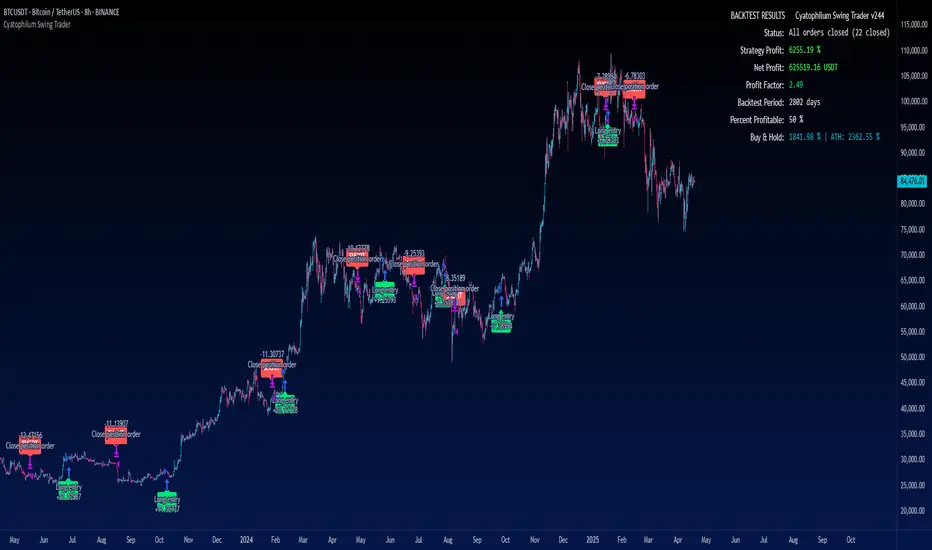
Cyatophilum Swing Trader [BACKTEST]This is an indicator for swing trading which allows you to build your own strategies, backtest and alert. This version is the backtest which allows to use the Strategy Tester. The alert version can be found in my profile scripts page.
The particularity of this indicator is that it contains several indicators, including a custom one, that you can choose in a drop down list, as well as a trailing stop loss and take profit system.
The current indicators are :
CYATO AI: a custom indicator inspired by Donchian Channels that will catch each big trend and important reversal points .
The indicator has two major "bands" or channels and two minor bands. The major bands are bigger and are always displayed.
When price reaches a major band, acting as a support/resistance, it will either bounce on it or break through it. This is how "tops" and "bottoms", and breakouts are caught.
The minor bands are used to catch smaller moves inside the major bands. A combination of volume, momentum and price action is used to calculate the signals.
Advantages of this indicator: it should catch top and bottoms better than other swing trade indicators.
Cons of this indicator: Some minor moves might be ignored. Sometimes the script will catch a fakeout due to the Bands design.
Best timeframes to use it : 2H~4H
Sample:
Other indicators available:
SARMA: A combination of Parabolic Stop and Reverse and Exponential Moving Average (20 and 40) .
SAR: Regular Parabolic Stop and Reverse .
QQE: An indicator based on Quantitative Qualitative Estimation .
SUPERTREND: A reversal indicator based on Average True Range .
CHANNELS: The classic Donchian Channels .
More indicators might be added in the future.
About the signals: each entry (long & short) is calculated at bar close to avoid repainting. Exits (SL & TP) can either be intra-bar or at bar close using the Exit alert type parameter.
STOP LOSS SYSTEM
The base indicators listed above can be used with or without TP/SL.
TP and SL can be both turned on and off and configured for both directions.
The system can be configured with 3 parameters as follows:
Stop Loss Base % Price: Starting Value for LONG/SHORT stop loss
Trailing Stop % Price to Trigger First parameter related to the trailing stop loss. Percentage of price movement in the right direction required to make the stop loss line move.
Trailing Stop % Price Movement: Second parameter related to the trailing stop loss. Percentage for the stop loss trailing movement.
Another option is the "Reverse order on Stop Loss". Use this if you want the strategy to trigger a reverse order when a stop loss is hit.
TAKE PROFIT SYSTEM
The system can be configured with 2 parameters as follows:
Take Profit %: Take profit value in percentage of price.
Trailing Profit Deviation %: Percent deviation for the trailing take profit.
Combining indicators and Take Profit/Stop Loss
One thing to note is that if a reversal signal triggers during a trade, the trade will be closed before SL or TP is reached.
Indeed, the base indicators are reversal indicators, they will trigger long/short signals to follow the trend.
It is possible to use a takeprofit without stop loss, like in this example, knowing that the signal will reverse if the trade goes badly.
The base indicators settings can be changed in the "Advanced Parameters" section.
Configuration used for this snapshot:
BACKTEST SETTINGS
· Initial Capital: 10 000 $
· Order Size: 10% equity (to avoid compounding effect)
· Commission : 0.1% per order (total commission paid: 244.41 €)
· Slippage: 5 ticks
Oldest trade: 2014-04-01
Backtest Period: From 2014-04-01 to 2020-09-04
Use the link below to obtain access to this indicator.
BO - Bar's direction Signal - BacktestingBO - Bar's direction Signal - Backtesting Options:
A. Factors Calculate probability of x bars same direction
1. Periods Counting: Data to count From day/month/year To day/month/year
2. Trading Time: only cases occurred in trading time were counted.
B. Timezone
1. Trading time depend on Time zone and specified chart.
2. Enable Highlight Trading Time to check your period time is correct
C. Date Backtesting
* Only cases occurred in Date Backtesting were reported.
D. Setup Options & Rule
1. Reversal after 2 bars same direction
* Probability of 3 bars same direction < 50
* 2 bars same direction is start of series
2. Reversal after 3 bars same direction
* Probability of 4 bars same direction < 50
* 3 bars same direction is start of series
3. Reversal after 4 bars same direction
* Probability of 4 bars same direction < 50
* 3 bars same direction is start of series
4. Reversal after 5 bars same direction
* Probability of 5 bars same direction < 50
* 4 bars same direction is start of series
5. Reversal after 6 bars same direction
* Probability of 6 bars same direction < 50
* 5 bars same direction is start of series

BITCOINDICATOR StrategyStrategy for BITCOINDICATOR for your own backtesting purposes.
The trade locations mirror the price label values generated by BITCOINDICATOR (You can check by clicking on Strategy Tester > List of Trades). Just like BITCOINDICATOR, this strategy works with all time frames, although higher time frames will result in better average profit per trade.
Inputs:
- Click the gear icon to adjust the backtesting date range inputs.
Properties (gear icon then click properties tab):
- The default initial capital is 0, and the default order size is 1 Contract (1 BTC ) per trade (this gives more weight to the most recent data).
* We recommend keeping the order size in contracts because if you use fiat, the time periods of lower-priced Bitcoin will have a greater impact on the strategy (since those trades would transact more BTC ).
- Pyramiding is the number of trades allowed to be taken in the same direction. The default value is set to 5, although it is rare to see more than 2 trades in the same direction.
* Additional trades in the same direction can be useful for adding on to your position or just for trend confirmation. If you prefer to see every SHORT followed by a LONG and vice-versa, you can change pyramiding to 1.
Side Notes:
- BITCOINDICATOR strategy can also be used for any Altcoin/Stable coin pair (such as ETH/USD). However, you will want to increase the order size from 1 Contract, to suit your Altcoin (For example, at the time of writing: 1 BTC = 47 ETH, so I would trade ETH/USD with an order size of 47 contracts). Of course, you can adjust the order size to the amount that you are actually trading.
- You will notice that the lower the selected time frame, the date range for backtesting becomes more limited. This is because there is a historical bar data limit of 5,000 - 10,000 bars depending on the tier of your TradingView account.
*Bitcoindicator Strategy is part of the Bitcoindicator package.
For detailed information on Bitcoindicator and how to add it to your charts, please visit:
www.bitcoindicator.com
Strategy tested on BTC/USD(Day) from 1/1/2017 - 10/1/2019 :

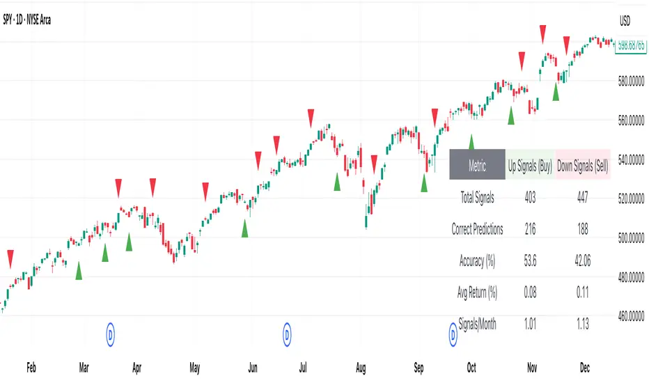
[DEM] Relative Strength Signal (With Backtesting) Relative Strength Signal (With Backtesting) is a momentum indicator that generates trading signals based on when an asset reaches its highest or lowest relative strength compared to the SPY benchmark over a 20-period lookback window. The indicator calculates relative strength by dividing the current asset's price by SPY's price, then triggers buy signals when this ratio hits a 20-period high (indicating maximum outperformance) and sell signals when it reaches a 20-period low (indicating maximum underperformance). To prevent signal clustering and improve practical utility, the indicator includes a built-in filter that requires a minimum number of bars (default 20) to pass between signals of the same type, ensuring adequate spacing for meaningful trade opportunities. The system includes comprehensive backtesting functionality that tracks signal accuracy, average returns, and signal frequency over time, displaying these performance metrics in a detailed statistics table to help traders evaluate the effectiveness of trading on relative strength extremes versus the broader market.

[DEM] Pullback Signal (With Backtesting) Pullback Signal (With Backtesting) is a sophisticated fractal-based indicator that identifies potential reversal opportunities by detecting swing highs and lows followed by pullback conditions in the opposite direction. The indicator uses complex fractal logic to identify pivot points where price forms a local high or low over a customizable period (default 3 bars), then generates buy signals when an upward fractal is identified and the current close is below the previous close, or sell signals when a downward fractal occurs and the current close is above the previous close. This approach captures the classic pullback scenario where price retraces after forming a swing point, potentially offering favorable risk-reward entry opportunities. The indicator includes comprehensive backtesting functionality that tracks signal accuracy, average returns, and signal frequency over time, displaying these performance metrics in a detailed statistics table to help traders evaluate the historical effectiveness of the pullback strategy across different market conditions.
[DEM] Multi-RSI Signal (With Backtesting) Multi-RSI Signal (With Backtesting) is a technical indicator that generates buy signals based on multiple RSI (Relative Strength Index) timeframes simultaneously reaching oversold conditions. The indicator monitors RSI values across seven different periods (2, 3, 4, 5, 6, 8, 25, 50, and 100) and triggers a buy signal only when all shorter-term RSIs (2-8 periods) drop below specific thresholds (mostly below 10-20) while longer-term RSIs (25, 50, 100) remain within defined ranges, indicating a confluence of oversold conditions across multiple timeframes. The system includes comprehensive backtesting capabilities that track signal accuracy, average returns, and signal frequency over time, displaying these performance metrics in a real-time statistics table. Unlike typical single-RSI approaches, this multi-timeframe methodology aims to filter out false signals by requiring alignment across various RSI periods, though it currently only generates buy signals with no corresponding sell signal logic implemented.

[DEM] Four RMA Signal (With Backtesting) Four RMA Signal (With Backtesting) is designed to generate buy and sell signals based on a hierarchical alignment of four Rolling Moving Averages (RMA) with periods of 200, 300, 400, and 500, combined with price action confirmation through the fastest RMA line. It also includes a comprehensive backtesting framework to evaluate the historical performance of these signals. The indicator overlays directly on the price chart, plotting signals and displaying performance statistics in a table. The strategy generates buy signals when all four RMAs are aligned in ascending order (200>300>400>500, indicating strong bullish momentum across multiple timeframes) and the low crosses above the 200-period RMA, while sell signals are triggered when the RMAs are aligned in descending order (200<300<400<500, indicating strong bearish momentum) and the high crosses below the 200-period RMA, ensuring signals only occur during periods of confirmed long-term directional bias with immediate price confirmation through the fastest moving average.

[DEM] Floating Reversal Signal (With Backtesting) Floating Reversal Signal (With Backtesting) is designed to identify potential reversal opportunities by detecting counter-trend momentum shifts using a combination of SuperTrend analysis, ATR-based candle size filtering, and RSI oversold/overbought conditions. It also includes a comprehensive backtesting framework to evaluate the historical performance of these signals. The indicator overlays directly on the price chart, plotting signals and displaying performance statistics in a table. The strategy generates buy signals when price forms a bullish candle during a SuperTrend downtrend, with the previous candle's body size falling within specified ATR multiplier ranges (default 0.5x to 2x) and RSI showing oversold conditions below a configurable threshold, while sell signals are triggered under opposite conditions during uptrends with overbought RSI readings, aiming to capture "floating" reversal setups where price temporarily moves against the prevailing trend before resuming in the original direction.

PnL Bubble [%] | Fractalyst1. What's the indicator purpose?
The PnL Bubble indicator transforms your strategy's trade PnL percentages into an interactive bubble chart with professional-grade statistics and performance analytics. It helps traders quickly assess system profitability, understand win/loss distribution patterns, identify outliers, and make data-driven strategy improvements.
How does it work?
Think of this indicator as a visual report card for your trading performance. Here's what it does:
What You See
Colorful Bubbles: Each bubble represents one of your trades
Blue/Cyan bubbles = Winning trades (you made money)
Red bubbles = Losing trades (you lost money)
Bigger bubbles = Bigger wins or losses
Smaller bubbles = Smaller wins or losses
How It Organizes Your Trades:
Like a Photo Album: Instead of showing all your trades at once (which would be messy), it shows them in "pages" of 500 trades each:
Page 1: Your first 500 trades
Page 2: Trades 501-1000
Page 3: Trades 1001-1500, etc.
What the Numbers Tell You:
Average Win: How much money you typically make on winning trades
Average Loss: How much money you typically lose on losing trades
Expected Value (EV): Whether your trading system makes money over time
Positive EV = Your system is profitable long-term
Negative EV = Your system loses money long-term
Payoff Ratio (R): How your average win compares to your average loss
R > 1 = Your wins are bigger than your losses
R < 1 = Your losses are bigger than your wins
Why This Matters:
At a Glance: You can instantly see if you're a profitable trader or not
Pattern Recognition: Spot if you have more big wins than big losses
Performance Tracking: Watch how your trading improves over time
Realistic Expectations: Understand what "average" performance looks like for your system
The Cool Visual Effects:
Animation: The bubbles glow and shimmer to make the chart more engaging
Highlighting: Your biggest wins and losses get extra attention with special effects
Tooltips: hover any bubble to see details about that specific trade.
What are the underlying calculations?
The indicator processes trade PnL data using a dual-matrix architecture for optimal performance:
Dual-Matrix System:
• Display Matrix (display_matrix): Bounded to 500 trades for rendering performance
• Statistics Matrix (stats_matrix): Unbounded storage for complete statistical accuracy
Trade Classification & Aggregation:
// Separate wins, losses, and break-even trades
if val > 0.0
pos_sum += val // Sum winning trades
pos_count += 1 // Count winning trades
else if val < 0.0
neg_sum += val // Sum losing trades
neg_count += 1 // Count losing trades
else
zero_count += 1 // Count break-even trades
Statistical Averages:
avg_win = pos_count > 0 ? pos_sum / pos_count : na
avg_loss = neg_count > 0 ? math.abs(neg_sum) / neg_count : na
Win/Loss Rates:
total_obs = pos_count + neg_count + zero_count
win_rate = pos_count / total_obs
loss_rate = neg_count / total_obs
Expected Value (EV):
ev_value = (avg_win × win_rate) - (avg_loss × loss_rate)
Payoff Ratio (R):
R = avg_win ÷ |avg_loss|
Contribution Analysis:
ev_pos_contrib = avg_win × win_rate // Positive EV contribution
ev_neg_contrib = avg_loss × loss_rate // Negative EV contribution
How to integrate with any trading strategy?
Equity Change Tracking Method:
//@version=6
strategy("Your Strategy with Equity Change Export", overlay=true)
float prev_trade_equity = na
float equity_change_pct = na
if barstate.isconfirmed and na(prev_trade_equity)
prev_trade_equity := strategy.equity
trade_just_closed = strategy.closedtrades != strategy.closedtrades
if trade_just_closed and not na(prev_trade_equity)
current_equity = strategy.equity
equity_change_pct := ((current_equity - prev_trade_equity) / prev_trade_equity) * 100
prev_trade_equity := current_equity
else
equity_change_pct := na
plot(equity_change_pct, "Equity Change %", display=display.data_window)
Integration Steps:
1. Add equity tracking code to your strategy
2. Load both strategy and PnL Bubble indicator on the same chart
3. In bubble indicator settings, select your strategy's equity tracking output as data source
4. Configure visualization preferences (colors, effects, page navigation)
How does the pagination system work?
The indicator uses an intelligent pagination system to handle large trade datasets efficiently:
Page Organization:
• Page 1: Trades 1-500 (most recent)
• Page 2: Trades 501-1000
• Page 3: Trades 1001-1500
• Page N: Trades to
Example: With 1,500 trades total (3 pages available):
• User selects Page 1: Shows trades 1-500
• User selects Page 4: Automatically falls back to Page 3 (trades 1001-1500)
5. Understanding the Visual Elements
Bubble Visualization:
• Color Coding: Cyan/blue gradients for wins, red gradients for losses
• Size Mapping: Bubble size proportional to trade magnitude (larger = bigger P&L)
• Priority Rendering: Largest trades displayed first to ensure visibility
• Gradient Effects: Color intensity increases with trade magnitude within each category
Interactive Tooltips:
Each bubble displays quantitative trade information:
tooltip_text = outcome + " | PnL: " + pnl_str +
"\nDate: " + date_str + " " + time_str +
"\nTrade #" + str.tostring(trade_number) + " (Page " + str.tostring(active_page) + ")" +
"\nRank: " + str.tostring(rank) + " of " + str.tostring(n_display_rows) +
"\nPercentile: " + str.tostring(percentile, "#.#") + "%" +
"\nMagnitude: " + str.tostring(magnitude_pct, "#.#") + "%"
Example Tooltip:
Win | PnL: +2.45%
Date: 2024.03.15 14:30
Trade #1,247 (Page 3)
Rank: 5 of 347
Percentile: 98.6%
Magnitude: 85.2%
Reference Lines & Statistics:
• Average Win Line: Horizontal reference showing typical winning trade size
• Average Loss Line: Horizontal reference showing typical losing trade size
• Zero Line: Threshold separating wins from losses
• Statistical Labels: EV, R-Ratio, and contribution analysis displayed on chart
What do the statistical metrics mean?
Expected Value (EV):
Represents the mathematical expectation per trade in percentage terms
EV = (Average Win × Win Rate) - (Average Loss × Loss Rate)
Interpretation:
• EV > 0: Profitable system with positive mathematical expectation
• EV = 0: Break-even system, profitability depends on execution
• EV < 0: Unprofitable system with negative mathematical expectation
Example: EV = +0.34% means you expect +0.34% profit per trade on average
Payoff Ratio (R):
Quantifies the risk-reward relationship of your trading system
R = Average Win ÷ |Average Loss|
Interpretation:
• R > 1.0: Wins are larger than losses on average (favorable risk-reward)
• R = 1.0: Wins and losses are equal in magnitude
• R < 1.0: Losses are larger than wins on average (unfavorable risk-reward)
Example: R = 1.5 means your average win is 50% larger than your average loss
Contribution Analysis (Σ):
Breaks down the components of expected value
Positive Contribution (Σ+) = Average Win × Win Rate
Negative Contribution (Σ-) = Average Loss × Loss Rate
Purpose:
• Shows how much wins contribute to overall expectancy
• Shows how much losses detract from overall expectancy
• Net EV = Σ+ - Σ- (Expected Value per trade)
Example: Σ+: 1.23% means wins contribute +1.23% to expectancy
Example: Σ-: -0.89% means losses drag expectancy by -0.89%
Win/Loss Rates:
Win Rate = Count(Wins) ÷ Total Trades
Loss Rate = Count(Losses) ÷ Total Trades
Shows the probability of winning vs losing trades
Higher win rates don't guarantee profitability if average losses exceed average wins
7. Demo Mode & Synthetic Data Generation
When using built-in sources (close, open, etc.), the indicator generates realistic demo trades for testing:
if isBuiltInSource(source_data)
// Generate random trade outcomes with realistic distribution
u_sign = prand(float(time), float(bar_index))
if u_sign < 0.5
v_push := -1.0 // Loss trade
else
// Skewed distribution favoring smaller wins (realistic)
u_mag = prand(float(time) + 9876.543, float(bar_index) + 321.0)
k = 8.0 // Skewness factor
t = math.pow(u_mag, k)
v_push := 2.5 + t * 8.0 // Win trade
Demo Characteristics:
• Realistic win/loss distribution mimicking actual trading patterns
• Skewed distribution favoring smaller wins over large wins
• Deterministic randomness for consistent demo results
• Includes jitter effects to prevent visual overlap
8. Performance Limitations & Optimizations
Display Constraints:
points_count = 500 // Maximum 500 dots per page for optimal performance
Pine Script v6 Limits:
• Label Count: Maximum 500 labels per indicator
• Line Count: Maximum 100 lines per indicator
• Box Count: Maximum 50 boxes per indicator
• Matrix Size: Efficient memory management with dual-matrix system
Optimization Strategies:
• Pagination System: Handle unlimited trades through 500-trade pages
• Priority Rendering: Largest trades displayed first for maximum visibility
• Dual-Matrix Architecture: Separate display (bounded) from statistics (unbounded)
• Smart Fallback: Automatic page clamping prevents empty displays
Impact & Workarounds:
• Visual Limitation: Only 500 trades visible per page
• Statistical Accuracy: Complete dataset used for all calculations
• Navigation: Use page input to browse through entire trade history
• Performance: Smooth operation even with thousands of trades
9. Statistical Accuracy Guarantees
Data Integrity:
• Complete Dataset: Statistics matrix stores ALL trades without limit
• Proper Aggregation: Separate tracking of wins, losses, and break-even trades
• Mathematical Precision: Pine Script v6's enhanced floating-point calculations
• Dual-Matrix System: Display limitations don't affect statistical accuracy
Calculation Validation:
// Verified formulas match standard trading mathematics
avg_win = pos_sum / pos_count // Standard average calculation
win_rate = pos_count / total_obs // Standard probability calculation
ev_value = (avg_win * win_rate) - (avg_loss * loss_rate) // Standard EV formula
Accuracy Features:
• Mathematical Correctness: Formulas follow established trading statistics
• Data Preservation: Complete dataset maintained for all calculations
• Precision Handling: Proper rounding and boundary condition management
• Real-Time Updates: Statistics recalculated on every new trade
10. Advanced Technical Features
Real-Time Animation Engine:
// Shimmer effects with sine wave modulation
offset = math.sin(shimmer_t + phase) * amp
// Dynamic transparency with organic flicker
new_transp = math.min(flicker_limit, math.max(-flicker_limit, cur_transp + dir * flicker_step))
• Sine Wave Shimmer: Dynamic glowing effects on bubbles
• Organic Flicker: Random transparency variations for natural feel
• Extreme Value Highlighting: Special visual treatment for outliers
• Smooth Animations: Tick-based updates for fluid motion
Magnitude-Based Priority Rendering:
// Sort trades by magnitude for optimal visual hierarchy
sort_indices_by_magnitude(values_mat)
• Largest First: Most important trades always visible
• Intelligent Sorting: Custom bubble sort algorithm for trade prioritization
• Performance Optimized: Efficient sorting for real-time updates
• Visual Hierarchy: Ensures critical trades never get hidden
Professional Tooltip System:
• Quantitative Data: Pure numerical information without interpretative language
• Contextual Ranking: Shows trade position within page dataset
• Percentile Analysis: Performance ranking as percentage
• Magnitude Scaling: Relative size compared to page maximum
• Professional Format: Clean, data-focused presentation
11. Quick Start Guide
Step 1: Add Indicator
• Search for "PnL Bubble | Fractalyst" in TradingView indicators
• Add to your chart (works on any timeframe)
Step 2: Configure Data Source
• Demo Mode: Leave source as "close" to see synthetic trading data
• Strategy Mode: Select your strategy's PnL% output as data source
Step 3: Customize Visualization
• Colors: Set positive (cyan), negative (red), and neutral colors
• Page Navigation: Use "Trade Page" input to browse trade history
• Visual Effects: Built-in shimmer and animation effects are enabled by default
Step 4: Analyze Performance
• Study bubble patterns for win/loss distribution
• Review statistical metrics: EV, R-Ratio, Win Rate
• Use tooltips for detailed trade analysis
• Navigate pages to explore full trade history
Step 5: Optimize Strategy
• Identify outlier trades (largest bubbles)
• Analyze risk-reward profile through R-Ratio
• Monitor Expected Value for system profitability
• Use contribution analysis to understand win/loss impact
12. Why Choose PnL Bubble Indicator?
Unique Advantages:
• Advanced Pagination: Handle unlimited trades with smart fallback system
• Dual-Matrix Architecture: Perfect balance of performance and accuracy
• Professional Statistics: Institution-grade metrics with complete data integrity
• Real-Time Animation: Dynamic visual effects for engaging analysis
• Quantitative Tooltips: Pure numerical data without subjective interpretations
• Priority Rendering: Intelligent magnitude-based display ensures critical trades are always visible
Technical Excellence:
• Built with Pine Script v6 for maximum performance and modern features
• Optimized algorithms for smooth operation with large datasets
• Complete statistical accuracy despite display optimizations
• Professional-grade calculations matching institutional trading analytics
Practical Benefits:
• Instantly identify system profitability through visual patterns
• Spot outlier trades and risk management issues
• Understand true risk-reward profile of your strategies
• Make data-driven decisions for strategy optimization
• Professional presentation suitable for performance reporting
Disclaimer & Risk Considerations:
Important: Historical performance metrics, including positive Expected Value (EV), do not guarantee future trading success. Statistical measures are derived from finite sample data and subject to inherent limitations:
• Sample Bias: Historical data may not represent future market conditions or regime changes
• Ergodicity Assumption: Markets are non-stationary; past statistical relationships may break down
• Survivorship Bias: Strategies showing positive historical EV may fail during different market cycles
• Parameter Instability: Optimal parameters identified in backtesting often degrade in forward testing
• Transaction Cost Evolution: Slippage, spreads, and commission structures change over time
• Behavioral Factors: Live trading introduces psychological elements absent in backtesting
• Black Swan Events: Extreme market events can invalidate statistical assumptions instantaneously

Candle AnalysisImportant Setup Note
Optimize Your Viewing Experience
To ensure the Candle Analysis Indicator displays correctly and to prevent any default chart colors from interfering with the indicator's visuals, please adjust your chart settings:
Right-Click on the Chart and select "Settings".
Navigate to the "Symbol" tab.
Set transparent default candle colors:
- Body
-Borders
- Wick
By customizing these settings, you'll experience the full visual benefits of the indicator without any overlapping colors or distractions.
Elevate your trading strategy with the Candle Analysis Indicator—a powerful tool designed to give you a focused view of the market exactly when you need it. Whether you're honing in on specific historical periods or testing new strategies, this indicator provides the clarity and control you've been looking for.
Key Features:
🔹 Custom Date Range Selection
Tailored Analysis: Choose your own start and end dates to focus on the market periods that matter most to you.
Historical Insights: Dive deep into past market movements to uncover hidden trends and patterns.
🔹 Dynamic Backtesting Simulation
Interactive Playback: Enable backtesting to simulate how the market unfolded over time.
Strategy Testing: Watch candles appear at your chosen interval, allowing you to test and refine your trading strategies in real-time scenarios.
🔹 Enhanced Visual Clarity
Focused Visualization: Only candles within your specified date range are highlighted, eliminating distractions from irrelevant data.
Distinct Candle Styling: Bullish and bearish candles are displayed with unique colors and transparency, making it easy to spot market sentiment at a glance.
🔹 User-Friendly Interface
Easy Setup: Simple input options mean you can configure the indicator quickly without any technical hassle.
Versatile Application: Compatible with various timeframes—whether you're trading intraday, daily, or weekly.
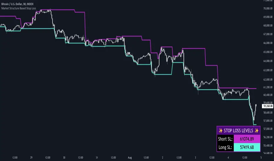
Market Structure Based Stop LossMarket Structure Based Dynamic Stop Loss
Introduction
The Market Structure Based Stop Loss indicator is a strategic tool for traders designed to be useful in both rigorous backtesting and live testing, by providing an objective, “guess-free” stop loss level. This indicator dynamically plots suggested stop loss levels based on market structure, and the concepts of “interim lows/highs.”
It provides a robust framework for managing risk in both long and short positions. By leveraging historical price movements and real time market dynamics, this indicator helps traders identify quantitatively consistent risk levels while optimizing trade returns.
Legend
This indicator utilizes various inputs to customize its functionality, including "Stop Loss Sensitivity" and "Wick Depth," which dictate how closely the stop loss levels hug the price's highs and lows. The stop loss levels are plotted as lines on the trading chart, providing clear visual cues for position management. As seen in the chart below, this indicator dynamically plots stop loss levels for both long and short positions at every point in time.
A “Stop Loss Table” is also included, in order to enhance precision trading and increase backtesting accuracy. It is customizable in both size and positioning.
Case Study
Methodology
The methodology behind this indicator focuses on the precision placement of stop losses using market structure as a guide. It calculates stop losses by identifying the "lowest close" and the corresponding "lowest low" for long setups, and inversely for short setups. By adjusting the sensitivity settings, traders can tweak the indicator's responsiveness to price changes, ensuring that the stop losses are set with a balance between tight risk control and enough room to avoid premature exits due to market noise. The indicator's ability to adapt to different trading styles and time frames makes it an essential tool for traders aiming for efficiency and effectiveness in their risk management strategies.
An important point to make is the fact that the stop loss levels are always placed within the wicks. This is important to avoid what can be described as a “floating stop loss”. A stop loss placed outside of a wick is susceptible to an outsized degree of slippage. This is because traders always cluster their stop losses at high/low wicks, and a stop loss placed outside of this level will inevitably be caught in a low liquidity cascade or “wash-out.” When price approaches a cluster of stop losses, it is highly probable that you will be stopped out anyway, so it is prudent to attempt to be the trader who gets stopped out first in order to avoid high slippage, and losses above what you originally intended.
// For long positions: stop-loss is slightly inside the lowest wick
float dynamic_SL_Long = lowestClose - (lowestClose - lowestLow) * (1 - WickDepth)
// For short positions: stop-loss is slightly inside the highest wick
float dynamic_SL_Short = highestClose + (highestHigh - highestClose) * (1 - WickDepth)
The percentage depth of the wick in which the stop loss is placed is customisable with the “Wick Depth” variable, in order to customize stop loss strategies around the liquidity of the market a trader is executing their orders in.
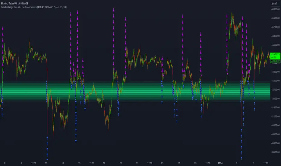
Hulk Grid Algorithm V2 - The Quant ScienceIt's the latest proprietary grid algorithm developed by our team. This software represents a clearer and more comprehensive modernization of the deprecated Hulk Grid Algorithm. In this new release, we have optimized the source code architecture and investment logic, which we will describe in detail below.
Overview
Hulk Grid Algorithm V2 is designed to optimize returns in sideways market conditions. In this scenario, the algorithm divides purchases with long orders at each level of the grid. Unlike a typical grid algorithm, this version applies an anti-martingale model to mitigate volatility and optimize the average entry price. Starting from the lower level, the purchase quantity is increased at each new subsequent level until reaching the upper level. The initial quantity of the first order is fixed at 0.50% of the initial capital. With each new order, the initial quantity is multiplied by a value equal to the current grid level (where 1 is the lower level and 10 is the upper level).
Example: Let's say we have an initial capital of $10,000. The initial capital for the first order would be $50 * 1 = $50, for the second order $50 * 2 = $100, for the third order $50 * 3 = $150, and so on until reaching the upper level.
All previously opened orders are closed using a percentage-based stop-loss and take-profit, calculated based on the extremes of the grid.
Set Up
As mentioned earlier, the user's goal is to analyze this strategy in markets with a lack of trend, also known as sideways markets. After identifying a price range within which the asset tends to move, the user can choose to create the grid by placing the starting price at the center of the range. This way, they can consider trading the asset, if the backtesting generates a return greater than the Buy & Hold return.
Grid Configuration
To create the grid, it's sufficient to choose the starting price during the launch phase. This level will be the center of the grid from which the upper and lower levels will be calculated. The grid levels are computed using an arithmetic method, adding and subtracting a configurable fixed amount from the user interface (Grid Step $).
Example: Let's imagine choosing 1000 as the starting price and 50 as the Grid Step ($). The upper levels will be 1000, 1050, 1100, 1150, 1200. The lower levels will be 950, 900, 850, 800, and 750.
Markets
This software can be used in all markets: stocks, indices, commodities, cryptocurrencies, ETFs, Forex, etc.
Application
With this backtesting software, is possible to analyze the strategy and search for markets where it can generate better performance than Buy & Hold returns. There are no alerts or automatic investment mechanisms, and currently, the strategy can only be executed manually.
Design
Is possible to modify the grid style and customize colors by accessing the Properties section of the user interface.
Hybrid, Zero lag, Adaptive cycle MACD Backtest (Simple) [Loxx]Simple backtest for Hybrid, Zero lag, Adaptive cycle MACD Backtest (Simple) found here:
What this backtest includes:
-Customization of inputs for MACD calculation
-Take profit 1 (TP1), and Stop-loss (SL), calculated using standard RMA-smoothed true range
-Activation of TP1 after entry candle closes
-Zero-cross entry signal plots
-MACD-Signal cross entry continuations
-Longs and shorts
Happy trading!

HMA (Hull Moving Averge) Backtest (Simple) [Loxx]Simple backtest for HMA (Hull Moving Average) found here:
What this indicator includes:
- Various average modes to fine-tune the signal
- Shift to offset chart (purely visual, has no bearing on actual calculation or backtest)
What this backtest includes:
-Longs and shorts
-Customization of inputs for HMA calculation
-Take profit 1 (TP1), and Stop-loss (SL), calculated using standard RMA-smoothed true range
-Activation of TP1 after entry candle closes
Happy trading!