Why Traders Prefer Momentum Strategies1. Understanding Momentum Trading
Momentum trading involves identifying securities that are moving significantly in one direction with high volume and capitalizing on the continuation of that trend. Unlike value investing, which focuses on fundamental valuation, momentum trading is primarily price action driven. Traders do not necessarily care about the intrinsic value of a stock; rather, they seek trends and patterns that indicate future price movement.
Momentum strategies can be applied across various time frames—from intraday scalping to long-term swing trading, making it versatile for traders with different risk appetites.
2. Behavioral Basis of Momentum
One reason traders prefer momentum strategies is that they align with human behavioral tendencies in financial markets. Two key behavioral biases drive momentum:
Herd Behavior: Investors tend to follow the crowd, buying assets that are trending upward or selling assets that are trending downward.
Overreaction and Underreaction: Markets often overreact to news or earnings, creating short-term trends that momentum traders exploit.
Momentum strategies allow traders to capitalize on these predictable psychological patterns, rather than attempting to forecast exact valuations or market turning points.
3. Technical Simplicity
Momentum trading is often technically straightforward to implement. Traders rely on indicators like:
Moving Averages (MA): Identifies the direction of the trend.
Relative Strength Index (RSI): Highlights overbought or oversold conditions.
MACD (Moving Average Convergence Divergence): Tracks momentum shifts.
Volume Indicators: Confirm trend strength.
These tools enable traders to quickly analyze market behavior, which makes momentum strategies appealing even to traders with limited experience.
4. High Profit Potential
One of the primary reasons traders prefer momentum strategies is the potential for high returns in short time frames. When a trend is strong, the profit potential can exceed what might be possible through traditional buy-and-hold strategies. By entering a trend early and exiting before it reverses, traders can maximize gains while limiting exposure to long-term market uncertainties.
5. Flexibility Across Market Conditions
Momentum strategies can be adapted to various market environments:
Bull Markets: Traders ride upward trends in growth stocks, indices, or sectors.
Bear Markets: Momentum traders can short-sell declining assets, profiting from negative trends.
Sideways Markets: Even in range-bound markets, momentum traders can use oscillators like RSI to capture mini-trends.
This adaptability makes momentum trading attractive in both rising and falling markets, unlike strategies that depend solely on market appreciation.
6. Speed and Agility
Modern traders have access to high-speed trading platforms and real-time market data, which makes momentum strategies feasible and efficient. Momentum traders can enter and exit positions within minutes or hours, exploiting price inefficiencies as they occur. This speed is particularly appealing to active traders who want rapid feedback on their strategies.
7. Empirical Evidence Supporting Momentum
Research in financial markets consistently shows that momentum strategies can produce positive abnormal returns over time. Studies by Jegadeesh and Titman (1993) and others indicate that:
Stocks that perform well over the past 3–12 months tend to outperform in the following months.
Momentum effects are observed globally across equities, commodities, and even cryptocurrencies.
The empirical evidence reinforces traders’ confidence in using momentum strategies as a reliable approach to capitalizing on trends.
8. Reduced Reliance on Fundamental Analysis
Momentum strategies appeal to traders who prefer technical over fundamental analysis. Instead of analyzing balance sheets, cash flows, or macroeconomic indicators, momentum traders focus on price and volume behavior, enabling:
Quicker decision-making
Simplified trade execution
Reduced exposure to complex financial statements
For traders who value speed and simplicity, this approach is far more practical.
9. Integration with Risk Management
Momentum trading can be systematically combined with risk management techniques, making it attractive for professional traders. Common methods include:
Stop-loss orders: Automatically exit losing trades.
Position sizing: Adjusting trade size according to volatility.
Trailing stops: Lock in profits as trends continue.
By pairing momentum strategies with disciplined risk control, traders can maximize upside potential while limiting downside risk.
10. Psychological Advantages
Momentum trading provides clear, objective entry and exit signals, which helps traders avoid emotional decision-making—a common pitfall in trading. Knowing when to buy or sell based on predefined criteria can reduce anxiety and hesitation, which is particularly valuable in fast-moving markets.
Additionally, successful momentum trades can reinforce trader confidence, creating a positive feedback loop that encourages disciplined execution of strategies.
11. Scalability Across Asset Classes
Momentum strategies are not limited to equities. Traders often apply momentum principles to:
Commodities (gold, oil)
Forex markets
Cryptocurrencies
ETFs and indices
This versatility makes momentum trading a universal tool, appealing to traders with diverse portfolios.
12. Drawbacks and Considerations
While momentum strategies are popular, traders must also be aware of potential pitfalls:
Trend Reversals: Momentum can fade abruptly, resulting in losses.
High Transaction Costs: Frequent trading can lead to increased brokerage and slippage.
Overcrowding: Popular momentum trades can attract many participants, reducing profitability.
Successful momentum traders mitigate these risks through strict discipline, risk management, and continuous monitoring.
13. Momentum in Algorithmic Trading
The rise of algorithmic and quantitative trading has amplified the appeal of momentum strategies. Algorithms can:
Detect micro-trends faster than humans
Execute trades in milliseconds
Adapt to changing market conditions
This has made momentum strategies even more efficient and profitable, particularly in high-frequency and institutional trading environments.
14. Conclusion
Traders prefer momentum strategies because they offer a combination of high-profit potential, technical simplicity, and adaptability across market conditions. Momentum trading aligns with human behavioral tendencies, leverages empirical evidence of trend persistence, and can be integrated with robust risk management practices. While not without challenges, the speed, scalability, and psychological clarity of momentum trading make it one of the most attractive strategies for traders ranging from retail investors to large institutional funds.
In essence, momentum trading capitalizes on the market’s natural tendencies to trend in patterns, allowing traders to ride waves of price action with discipline, precision, and profitability.
Chart Patterns
The Power of Mindset in Trading Success1. Understanding Trading Mindset
The term "trading mindset" refers to the set of psychological attitudes, beliefs, and emotional controls that guide a trader's decision-making process. It encompasses a trader's ability to manage stress, stick to strategies, control impulses, learn from mistakes, and maintain a positive and disciplined approach. Unlike technical skills, which can be learned through study and practice, the trading mindset is a continual development process that evolves with experience.
A healthy trading mindset is not about eliminating emotions but rather mastering them. Traders who can observe their feelings without being controlled by them are better equipped to make rational, objective decisions even under pressure. Emotional self-awareness, resilience, patience, and confidence are key traits of a successful trading mindset.
2. Emotional Challenges in Trading
Financial markets are inherently uncertain and unpredictable. Traders face constant challenges such as price volatility, unexpected news events, and losses that can test emotional fortitude. Several emotional challenges can hinder trading performance:
Fear: Fear is a common emotion that can prevent traders from taking opportunities or cause premature exits from profitable trades. It can stem from fear of losing money, fear of missing out (FOMO), or fear of being wrong.
Greed: Greed can drive traders to overtrade, take excessive risks, or hold positions longer than prudent. The desire for higher profits can overshadow rational decision-making.
Regret: Traders may dwell on past mistakes or missed opportunities, which can affect confidence and lead to reactive trading decisions.
Overconfidence: Experiencing a winning streak can make traders overconfident, causing them to deviate from their strategy and risk larger losses.
Understanding and managing these emotional states is critical to sustaining long-term trading success. Emotional discipline ensures that decisions are guided by strategy rather than impulses.
3. The Role of Discipline
Discipline is the backbone of a successful trading mindset. Even the best strategies will fail if a trader cannot adhere to rules regarding entry, exit, and risk management. Discipline in trading manifests in several ways:
Following a Trading Plan: A trading plan outlines strategies, risk parameters, and trade management rules. Traders with strong discipline stick to this plan consistently, avoiding impulsive decisions.
Risk Management: Proper position sizing, stop-loss levels, and capital allocation are essential to protect against catastrophic losses. A disciplined trader respects risk parameters even in emotionally charged market conditions.
Consistency: Markets fluctuate, but disciplined traders maintain a consistent approach to analysis, execution, and evaluation. Consistency reduces the impact of random market movements on psychological stability.
Discipline is cultivated over time and is often tested in moments of stress. Successful traders develop habits and routines that reinforce disciplined behavior, such as journaling trades, reviewing performance, and maintaining clear decision-making processes.
4. Growth Mindset vs. Fixed Mindset
The concept of mindset, popularized by psychologist Carol Dweck, can be applied directly to trading. Traders with a growth mindset view challenges, losses, and mistakes as opportunities to learn and improve. They embrace feedback, adapt to changing market conditions, and see setbacks as temporary hurdles. Conversely, traders with a fixed mindset may view losses as personal failures, resist learning, and struggle to adapt.
A growth mindset in trading leads to several advantages:
Continuous Learning: Markets evolve, and successful traders continually educate themselves about new strategies, instruments, and market dynamics.
Adaptability: Traders with a growth mindset adjust their methods in response to market changes, avoiding rigid adherence to outdated strategies.
Resilience: Viewing losses as learning experiences reduces emotional stress and helps traders recover more quickly from setbacks.
5. Psychological Biases and Their Impact
Cognitive biases can subtly influence trading decisions, often without conscious awareness. Understanding these biases is essential for developing a strong trading mindset:
Confirmation Bias: Traders may seek information that supports their preconceptions and ignore contradictory data, leading to poor decision-making.
Loss Aversion: The tendency to fear losses more than valuing equivalent gains can result in holding losing positions too long or exiting winning trades prematurely.
Recency Bias: Recent events may disproportionately influence decisions, causing traders to overemphasize short-term trends rather than considering long-term patterns.
Herd Mentality: Following the crowd can lead to impulsive decisions and market bubbles. Independent thinking and critical analysis help counteract this bias.
By recognizing and mitigating these biases, traders can make more objective, rational, and profitable decisions.
6. Developing Mental Resilience
Resilience is the ability to recover from setbacks and remain focused on long-term goals. In trading, mental resilience allows individuals to:
Handle Losses: Losses are inevitable in trading. Resilient traders analyze mistakes without self-blame and use them as lessons for improvement.
Maintain Confidence: Confidence in one’s strategy and skills prevents panic-driven decisions and promotes patience during drawdowns.
Control Stress: High-pressure environments can trigger stress and anxiety. Resilient traders use techniques such as mindfulness, meditation, or deep breathing to maintain composure.
Resilience is not innate; it can be strengthened through deliberate practice, reflection, and psychological conditioning.
7. The Importance of Patience
Patience is a critical trait in trading. Successful traders wait for the right setups rather than chasing the market. Impatience can lead to overtrading, premature exits, or taking trades that do not fit the strategy. Cultivating patience involves:
Trusting the Process: Believing in your analysis and strategy allows you to wait for optimal trade opportunities.
Avoiding Impulsive Decisions: Emotional reactions often result in losses. Patience ensures that trades are executed based on logic and analysis rather than temporary market fluctuations.
Long-Term Perspective: Traders with a long-term mindset focus on cumulative performance rather than short-term outcomes, reducing stress and impulsive behavior.
8. Visualization and Mental Preparation
Many successful traders use visualization techniques to reinforce a positive trading mindset. Visualization involves mentally rehearsing trades, imagining successful execution, and preparing for potential challenges. Benefits include:
Reducing Anxiety: Anticipating potential scenarios reduces emotional reactions during actual trades.
Enhancing Focus: Visualization reinforces clarity of strategy and decision-making under pressure.
Building Confidence: Mentally experiencing success boosts confidence and reinforces disciplined behavior.
Mental preparation, combined with regular reflection and journaling, strengthens a trader’s ability to navigate markets effectively.
9. Balancing Emotion and Logic
While technical and fundamental analysis provides a logical framework, emotions are an inseparable part of trading. The key to success lies in balance:
Emotional Awareness: Recognizing feelings such as fear, greed, or frustration helps traders respond consciously rather than react impulsively.
Rational Decision-Making: Logic-based decisions ensure consistency and reduce the influence of temporary emotions.
Adaptation: Markets are dynamic, and emotions sometimes signal real opportunities or risks. Effective traders integrate emotional insights with rational strategies.
10. Continuous Self-Reflection and Improvement
Trading success is not static. Even experienced traders must continually evaluate performance, adapt strategies, and refine their mindset. Self-reflection helps in:
Identifying Weaknesses: Recognizing recurring emotional or behavioral patterns that affect trading.
Reinforcing Strengths: Building on habits and traits that contribute to consistent success.
Enhancing Decision-Making: Learning from past trades improves judgment and reduces mistakes over time.
Maintaining a trading journal, seeking mentorship, and engaging in peer discussions can accelerate the development of a robust trading mindset.
11. Mindset and Risk Management
A strong mindset directly influences risk management, which is crucial for survival in trading. Traders with a resilient and disciplined mindset:
Stick to predetermined risk levels even during volatile market conditions.
Avoid overleveraging or taking impulsive positions.
Accept small losses without emotional turmoil, understanding that preservation of capital is essential for long-term success.
Mindset shapes how a trader perceives risk, allowing for calculated decisions rather than emotional gambles.
12. Real-Life Examples of Mindset Impact
Countless traders have demonstrated that mindset often outweighs technical skill in determining success:
Warren Buffett emphasizes patience, emotional control, and long-term thinking rather than rapid, high-risk trades.
Professional day traders often stress the importance of discipline, emotional awareness, and learning from mistakes over short-term technical mastery.
Historical trading failures often result from psychological lapses, such as panic-selling during downturns or overconfidence during market euphoria.
These examples reinforce the principle that trading success is as much about psychological preparation as analytical ability.
13. Strategies to Strengthen Trading Mindset
Building a robust trading mindset is an ongoing process. Effective strategies include:
Develop a Trading Plan: Clear guidelines reduce emotional decision-making.
Practice Mindfulness: Meditation and breathing techniques enhance focus and reduce stress.
Set Realistic Goals: Achievable targets prevent disappointment and emotional swings.
Journal Your Trades: Reflecting on decisions and outcomes improves self-awareness.
Learn from Mistakes: Treat losses as feedback rather than personal failure.
Maintain Work-Life Balance: Physical and mental well-being support cognitive function and emotional stability.
14. Conclusion
The power of mindset in trading success cannot be overstated. While technical analysis, strategies, and market knowledge provide the tools for trading, the psychological aspect determines how effectively those tools are applied. A strong trading mindset combines discipline, emotional control, patience, resilience, and continuous learning. Traders who cultivate these traits are better equipped to navigate market volatility, manage risk, and achieve consistent profitability.
Ultimately, trading is a test of character as much as skill. Success is rarely about luck; it is the result of mental fortitude, self-awareness, and the ability to make rational decisions under pressure. By prioritizing mindset development, traders can unlock their true potential, turning challenges into opportunities and navigating the financial markets with confidence, discipline, and long-term success.
Option Greeks and Advanced Hedging Strategies1. Introduction to Option Greeks
Options are derivative instruments that derive their value from an underlying asset, such as stocks, indices, commodities, or currencies. Unlike equities, the price of an option depends on several factors, including the underlying asset's price, volatility, time to expiration, and interest rates. Option Greeks quantify how sensitive an option’s price is to these variables, offering actionable insights into risk management.
There are five primary Greeks: Delta, Gamma, Theta, Vega, and Rho. Each provides a unique perspective on the risks and potential rewards associated with holding an option. Understanding these Greeks is critical for designing hedging strategies, structuring trades, and managing portfolio exposure.
2. Delta (Δ): Price Sensitivity to the Underlying
Delta measures the sensitivity of an option’s price to a $1 change in the price of the underlying asset. It ranges from 0 to 1 for call options and -1 to 0 for put options.
Call Options: Delta ranges from 0 to +1. A delta of 0.5 implies that if the underlying asset rises by $1, the option’s price will increase by $0.50.
Put Options: Delta ranges from -1 to 0. A delta of -0.5 indicates that a $1 increase in the underlying asset decreases the put option’s price by $0.50.
Delta also represents the probability of an option expiring in-the-money (ITM). For example, a delta of 0.7 suggests a 70% chance of finishing ITM. Traders use delta to gauge directional exposure, and delta can also serve as a foundational element in hedging strategies such as delta-neutral hedging, which will be discussed later.
3. Gamma (Γ): Rate of Change of Delta
Gamma measures the rate of change of delta in response to a $1 change in the underlying asset. While delta provides a linear approximation, gamma accounts for the curvature of option pricing.
High gamma indicates that delta can change significantly with small movements in the underlying asset, which is common for at-the-money (ATM) options nearing expiration.
Low gamma implies more stable delta, typical of deep-in-the-money (ITM) or far-out-of-the-money (OTM) options.
Gamma is crucial for traders managing delta-neutral portfolios. A high gamma position requires frequent rebalancing to maintain neutrality, as the delta shifts rapidly with price movements.
4. Theta (Θ): Time Decay of Options
Theta measures the sensitivity of an option’s price to the passage of time, assuming all other factors remain constant. Time decay is especially significant for options traders, as options lose value as expiration approaches.
Long options (buying calls or puts) have negative theta, meaning they lose value over time.
Short options (selling calls or puts) have positive theta, benefiting from the erosion of time value.
Theta is a critical factor in strategies such as calendar spreads or short straddles, where time decay can be exploited to generate profit.
5. Vega (ν): Sensitivity to Volatility
Vega measures an option’s sensitivity to changes in the volatility of the underlying asset. Volatility reflects market uncertainty; higher volatility increases the probability that an option will expire ITM, thus raising its premium.
Long options benefit from rising volatility (positive vega).
Short options benefit from declining volatility (negative vega).
Understanding vega is essential for strategies like straddles, strangles, and volatility spreads, where traders aim to profit from changes in implied volatility rather than directional price movements.
6. Rho (ρ): Sensitivity to Interest Rates
Rho measures the sensitivity of an option’s price to changes in the risk-free interest rate. While often overlooked in equity options due to low short-term interest rate fluctuations, rho becomes important for long-dated options (LEAPS) or currency options.
Call options increase in value with rising interest rates (positive rho).
Put options decrease in value with rising interest rates (negative rho).
Rho is generally less significant for short-term trading but critical for interest rate-sensitive instruments.
7. Combining Greeks for Holistic Risk Management
Individually, each Greek provides insight into one risk factor. However, professional traders consider them collectively to understand an option's total risk profile.
Delta addresses directional risk.
Gamma adjusts for changes in delta.
Theta manages time decay exposure.
Vega quantifies volatility risk.
Rho handles interest rate risk.
By monitoring these Greeks, traders can develop robust hedging strategies that dynamically adjust to market conditions.
8. Advanced Hedging Strategies
Hedging in options trading involves taking positions that offset risk in an underlying asset or portfolio. Advanced strategies often combine multiple Greeks to achieve delta-neutral, gamma-neutral, or vega-sensitive hedges, minimizing exposure to adverse market movements.
8.1 Delta-Neutral Hedging
Delta-neutral strategies aim to neutralize the directional exposure of a portfolio. Traders adjust their positions in the underlying asset or options to achieve a net delta of zero.
Example: Holding a long call option (delta = 0.6) and shorting 60 shares of the underlying stock (delta = -1 per share) results in a delta-neutral position.
Benefits: Protects against small price movements, ideal for traders who want to profit from volatility or time decay.
Limitations: Requires frequent rebalancing, especially with high gamma positions.
8.2 Gamma Hedging
Gamma hedging focuses on controlling the rate of change of delta. High gamma positions can result in delta swings, exposing traders to unexpected losses.
Traders achieve gamma neutrality by combining options with offsetting gamma values.
Example: A long ATM call (high gamma) may be hedged with OTM calls or puts to stabilize delta changes.
Benefits: Provides stability for delta-neutral portfolios.
Limitations: Complex to implement and can involve high transaction costs.
8.3 Vega Hedging
Vega hedging mitigates volatility risk. Traders who expect volatility to fall may sell options (short vega) while hedging long options (positive vega) to offset exposure.
Example: A trader long on an option may sell a different option with similar vega exposure to create a neutral vega position.
Benefits: Protects against unexpected spikes or drops in implied volatility.
Limitations: Requires deep understanding of options pricing and volatility behavior.
8.4 Theta Management and Calendar Spreads
Theta management involves leveraging time decay to generate income while maintaining a controlled risk profile.
Calendar spreads involve buying long-dated options and selling short-dated options on the same underlying asset.
Traders profit as the short-term option decays faster than the long-term option, benefiting from positive theta differential.
Benefits: Generates steady income and exploits time decay patterns.
Limitations: Sensitive to volatility changes, requiring careful vega management.
8.5 Multi-Greek Hedging
Professional traders often hedge portfolios using combinations of Greeks to achieve a multi-dimensional hedge.
Delta-Gamma-Vega Hedging: Neutralizes directional risk, delta swings, and volatility exposure simultaneously.
Useful for institutional traders managing large, complex portfolios where single-Greek hedges are insufficient.
Requires continuous monitoring and dynamic rebalancing to adapt to changing market conditions.
9. Practical Considerations in Hedging
While advanced Greek-based hedging strategies offer theoretical precision, practical implementation involves challenges:
Transaction Costs: Frequent rebalancing and multiple trades can reduce profitability.
Liquidity Risk: Some options may lack sufficient market liquidity, complicating execution.
Model Risk: Greeks are derived from mathematical models like Black-Scholes; real-world deviations can affect hedging effectiveness.
Market Gaps: Sudden, large price moves may bypass delta or gamma adjustments, leading to losses.
Traders must weigh the trade-offs between hedge precision and operational feasibility.
10. Real-World Applications
Option Greeks and hedging strategies are widely used in various contexts:
Institutional Portfolios: Delta-gamma-vega hedges protect large portfolios from market shocks.
Volatility Trading: Traders exploit implied vs. realized volatility differences using vega strategies.
Income Generation: Theta-positive strategies like covered calls and credit spreads provide steady cash flows.
Risk Management: Corporations with exposure to commodity prices or foreign exchange rates use option hedges to stabilize earnings.
11. Conclusion
Option Greeks are indispensable tools for understanding and managing the risks inherent in options trading. They provide a quantitative framework for measuring price sensitivity to underlying asset movements, time decay, volatility changes, and interest rates. Advanced hedging strategies leverage these Greeks to create positions that mitigate directional, volatility, and time-related risks.
While Greek-based hedging can be complex, the benefits are substantial: enhanced risk control, improved portfolio stability, and the ability to profit in diverse market conditions. Success requires a deep understanding of each Greek, continuous monitoring of market dynamics, and a disciplined approach to portfolio management. By mastering Option Greeks and advanced hedging strategies, traders gain a powerful edge in navigating the sophisticated world of derivatives trading.
Understanding Equity Market Structure in IndiaIntroduction
The equity market, often called the stock market, serves as the backbone of a country’s financial ecosystem. In India, it represents the vibrant and ever-evolving marketplace where companies raise capital and investors participate in wealth creation. Understanding the equity market structure in India is essential for anyone involved in trading, investing, or policymaking. It provides insight into how the market operates, who its participants are, how securities are traded, and how regulation ensures transparency and fairness.
India’s equity market has come a long way—from physical trading floors in the 1980s to a fully electronic, globally integrated system today. The structure comprises various layers, institutions, and participants, each performing specific roles to ensure the efficient functioning of the capital market.
1. Evolution of the Indian Equity Market
The Indian stock market has a rich history dating back to the 19th century when the Bombay Stock Exchange (BSE) was established in 1875. Initially, trading was informal, conducted under banyan trees in Mumbai by a group of brokers. However, with the liberalization of the Indian economy in 1991, the market witnessed modernization and rapid growth.
The introduction of the National Stock Exchange (NSE) in 1992 brought electronic trading, transparency, and efficiency. The Securities and Exchange Board of India (SEBI), formed in 1988 and granted statutory powers in 1992, became the principal regulator ensuring investor protection and market discipline. Today, India boasts one of the most advanced and liquid equity markets among emerging economies.
2. Structure of the Indian Equity Market
The Indian equity market operates through a two-tier structure:
Primary Market – where companies issue new shares to raise capital.
Secondary Market – where existing shares are traded among investors.
Let’s explore each in detail.
(a) The Primary Market
The primary market facilitates capital formation. Companies issue securities for the first time through Initial Public Offerings (IPOs), Follow-on Public Offers (FPOs), or Rights Issues. Investors purchase shares directly from the issuing company, and the proceeds are used for business expansion, debt repayment, or diversification.
Key participants include:
Issuing companies
Merchant bankers
Underwriters
Registrars
Investors
Regulation of the primary market is handled by SEBI, which ensures full disclosure of financial information, proper valuation, and transparent allotment processes. The IPO process in India involves book-building, anchor investors, and electronic bidding through platforms like ASBA (Application Supported by Blocked Amount).
(b) The Secondary Market
Once shares are listed on exchanges, they become tradable in the secondary market. Here, investors buy and sell shares through brokers on recognized exchanges such as NSE and BSE. The secondary market ensures liquidity and continuous price discovery.
Trades occur electronically through order-matching systems, with prices determined by demand and supply. This digital infrastructure has enhanced speed, accuracy, and transparency.
3. Major Stock Exchanges in India
India’s equity trading primarily occurs on two major exchanges:
(a) Bombay Stock Exchange (BSE)
Founded in 1875, BSE is Asia’s oldest exchange and one of the fastest in the world. Its benchmark index, SENSEX, tracks the performance of 30 top companies representing key sectors of the Indian economy. The BSE provides a wide range of products including equities, mutual funds, derivatives, and debt instruments.
(b) National Stock Exchange (NSE)
Established in 1992, NSE revolutionized Indian trading by introducing a fully automated, screen-based trading system. Its benchmark index, NIFTY 50, reflects the performance of the top 50 companies listed on the exchange. NSE is the largest exchange in India by trading volume and market capitalization.
Other regional exchanges such as Calcutta Stock Exchange (CSE) and Metropolitan Stock Exchange (MSE) exist but play a minor role compared to NSE and BSE.
4. Key Participants in the Indian Equity Market
The structure of the equity market is defined by the roles of various participants who ensure smooth operations.
(a) Investors
Investors are the backbone of the equity market and include:
Retail investors – individuals investing small amounts.
High Net-Worth Individuals (HNIs) – individuals with significant investable wealth.
Institutional investors – such as Mutual Funds, Pension Funds, Insurance Companies, and Foreign Portfolio Investors (FPIs).
(b) Brokers and Sub-brokers
Brokers are SEBI-registered members of exchanges who facilitate trading on behalf of clients. Sub-brokers operate under registered brokers to provide localized access to investors.
(c) Market Makers and Dealers
Market makers ensure liquidity by providing continuous buy and sell quotes. Dealers, on the other hand, trade securities on their own account.
(d) Depositories and Depository Participants (DPs)
India has two main depositories:
NSDL (National Securities Depository Limited)
CDSL (Central Depository Services Limited)
These institutions hold securities in dematerialized (Demat) form and facilitate the electronic transfer of ownership. DPs act as intermediaries between investors and depositories.
(e) Clearing Corporations
Entities like the National Securities Clearing Corporation Limited (NSCCL) and Indian Clearing Corporation Limited (ICCL) manage trade settlement, ensuring that funds and securities are exchanged efficiently and securely.
(f) Regulators
The Securities and Exchange Board of India (SEBI) regulates the equity market, ensuring transparency, investor protection, and compliance. The Reserve Bank of India (RBI) and Ministry of Finance also play supportive regulatory roles.
5. Trading Mechanism and Settlement Process
The Indian equity market uses an order-driven, automated trading system where buyers and sellers place orders through brokers using trading terminals.
Steps in the Trading Process:
Placing the order – The investor instructs the broker to buy or sell shares.
Order matching – The exchange’s electronic system matches buy and sell orders based on price and time priority.
Trade confirmation – Once matched, the trade is confirmed and recorded.
Clearing and settlement – Managed by clearing corporations.
India follows a T+1 settlement cycle (trade plus one business day).
Shares are credited to the buyer’s Demat account, and funds are transferred to the seller’s account.
This efficient system ensures minimal counterparty risk and prompt settlement.
6. Market Segments within the Equity Market
The equity market in India can be divided into various segments:
(a) Cash Market
Here, stocks are bought and sold for immediate delivery. The buyer gains ownership immediately after settlement.
(b) Derivatives Market
This includes trading in Futures and Options (F&O) contracts, where traders speculate on price movements or hedge risk. The derivative market in India has grown exponentially, making NSE one of the largest F&O exchanges globally.
(c) Institutional Trading Platforms (ITPs)
These allow unlisted companies, particularly startups, to raise capital and trade shares among institutional investors before going for a full IPO.
7. Indices and Market Benchmarks
Indices serve as barometers for market performance. The two most tracked indices are:
BSE SENSEX – tracks 30 large, financially sound companies.
NSE NIFTY 50 – represents 50 top companies across sectors.
Other sectoral and thematic indices include:
NIFTY Bank, NIFTY IT, NIFTY FMCG, etc.
These help investors gauge performance in specific industries.
8. Regulatory Framework
(a) Role of SEBI
SEBI’s mission is to protect investors, regulate intermediaries, and promote market development. Its major functions include:
Ensuring fair practices in IPOs and secondary market trading.
Monitoring insider trading and market manipulation.
Registering and supervising intermediaries like brokers, merchant bankers, and portfolio managers.
Implementing investor grievance mechanisms.
(b) Other Regulatory Bodies
RBI regulates capital inflows and outflows.
Ministry of Corporate Affairs (MCA) oversees corporate governance.
Stock Exchanges enforce listing obligations and compliance norms.
9. Technological Advancements and Digitalization
Technology has transformed the Indian equity market, making it more accessible and efficient.
Key innovations include:
Online trading platforms like Zerodha, Groww, and Upstox democratized investing for retail participants.
Algorithmic trading and High-Frequency Trading (HFT) increased liquidity and efficiency.
Mobile-based trading enabled real-time market participation.
Blockchain and AI tools are emerging for risk analysis and settlement processes.
The transition to a T+1 settlement cycle and the potential move toward instant settlement (T+0) further demonstrate India’s leadership in market modernization.
10. Foreign Participation and Global Integration
India’s equity market attracts global investors due to its growth potential, regulatory transparency, and robust infrastructure. Foreign Portfolio Investors (FPIs) play a key role, bringing in capital and global best practices.
FPIs invest in listed equities and debt instruments, regulated by SEBI.
Foreign Direct Investment (FDI), on the other hand, involves long-term investments in companies.
Global indices such as MSCI and FTSE include Indian equities, enhancing international visibility and liquidity.
11. Challenges in the Indian Equity Market
Despite its progress, the Indian equity market faces challenges such as:
Market volatility due to global economic uncertainty.
Low financial literacy among retail investors.
Corporate governance issues in some listed firms.
Regulatory complexity for foreign investors.
High concentration of trading in a few large-cap stocks.
Efforts by SEBI, stock exchanges, and financial institutions aim to address these challenges through education, transparency, and inclusive market policies.
12. Future Outlook of the Indian Equity Market
The future of India’s equity market looks promising. Several trends indicate robust growth potential:
Increased retail participation fueled by digital access and financial awareness.
Integration with global markets through international listings and GIFT City initiatives.
Expansion of derivative and SME platforms enhancing depth and liquidity.
Sustainable and ESG investing gaining traction among institutional investors.
AI-driven analytics reshaping trading strategies and investment decisions.
With India projected to become the world’s third-largest economy, its equity market will play a pivotal role in channeling capital to productive sectors and driving economic growth.
Conclusion
The Indian equity market is a dynamic and well-regulated system that has evolved into a cornerstone of the country’s financial stability and economic expansion. Its structure—comprising the primary and secondary markets, diverse participants, robust exchanges, and stringent regulatory oversight—ensures efficient capital allocation, investor protection, and continuous innovation.
From the traditional trading floors of the Bombay Stock Exchange to the algorithm-driven platforms of the modern era, India’s equity market reflects a journey of progress, resilience, and transformation. As digitalization, globalization, and financial inclusion continue to advance, the market’s structure will further strengthen, making it a global benchmark for transparency and growth in emerging economies.
Introduction to High Time Frame (HTF) Trading1. Understanding the Concept of High Time Frame (HTF) Trading
High Time Frame (HTF) trading is an approach where traders base their decisions on higher-duration charts such as the daily (1D), weekly (1W), or monthly (1M) time frames. Unlike short-term traders who focus on intraday fluctuations or minute-to-minute changes, HTF traders analyze the broader market structure to identify long-term trends, key support and resistance levels, and major reversals.
The goal of HTF trading is to align trades with the dominant market trend while minimizing the impact of short-term volatility and noise. It is a strategy favored by swing traders, position traders, and long-term investors who prefer a more patient, structured, and disciplined approach to market participation.
In essence, HTF trading is not about predicting short-term price movements but about understanding the bigger picture of market direction and trading with higher conviction.
2. The Importance of Time Frames in Trading
In trading, time frames determine how data is visualized on a chart. Each candlestick or bar represents a specific duration of price activity. For instance, in a 1-hour chart, each candle shows the open, high, low, and close within that hour. Similarly, in a weekly chart, each candle represents the price action of an entire week.
The choice of time frame shapes the trader’s strategy:
Low Time Frames (LTFs) – like 1-minute, 5-minute, or 15-minute charts – are used by scalpers and intraday traders for quick trades and small profits.
Medium Time Frames (MTFs) – such as 1-hour or 4-hour charts – help swing traders capture short-term trends.
High Time Frames (HTFs) – such as daily, weekly, or monthly charts – provide a broader perspective and are used for long-term decision-making.
HTF charts filter out random market noise and reveal the true structure of market trends. They act as a foundation for all forms of trading because even intraday traders benefit from understanding the dominant HTF trend.
3. Why Traders Choose High Time Frame Trading
HTF trading appeals to many traders for several reasons:
a) Clearer Market Structure
High time frames help traders see the overall direction of the market without being distracted by short-term fluctuations. Trends, consolidations, and reversals are easier to identify, enabling traders to make more informed and less emotional decisions.
b) Reduced Market Noise
Lower time frames are filled with false signals caused by random volatility. HTF trading eliminates much of this noise, allowing traders to focus on significant price action and key technical levels.
c) Stronger Trade Signals
Signals that appear on higher time frames – such as breakouts, moving average crossovers, or candlestick patterns – tend to be more reliable. For example, a bullish engulfing pattern on the daily chart holds more weight than the same pattern on a 5-minute chart.
d) Better Risk-to-Reward Ratios
HTF setups generally offer wider stop-loss levels but also much larger potential profits. Traders can capture multi-day or multi-week trends rather than short bursts of volatility.
e) Less Screen Time
Unlike day traders who need to monitor charts constantly, HTF traders can analyze the market once or twice a day. This suits those with full-time jobs or other commitments, making it a more flexible trading style.
4. The Core Principles of HTF Trading
To trade effectively on higher time frames, traders must follow certain foundational principles:
a) Patience
HTF trading requires patience because setups take time to form. A trader might wait several days or weeks for the ideal entry point, but the reward is typically worth the wait.
b) Trend Alignment
Trading with the trend is crucial in HTF analysis. Identifying whether the market is in an uptrend, downtrend, or consolidation phase helps avoid low-probability trades.
c) Multi-Time Frame Confirmation
Even in HTF trading, traders often combine multiple time frames to confirm trends. For example, a trader might use the weekly chart to identify the main trend and the daily chart to find entry points.
d) Risk Management
Since trades are held for longer durations, position sizing and stop-loss placement become critical. Traders must calculate their risk carefully, as drawdowns can be larger on higher time frames.
e) Emotional Discipline
HTF traders must stay disciplined and avoid overreacting to intraday market fluctuations. Emotional resilience is key because trades can take time to mature.
5. Commonly Used High Time Frames
HTF traders typically analyze the following charts:
Daily Chart (1D): Used to capture trends lasting from a few days to several weeks. It’s the most popular time frame for swing traders.
Weekly Chart (1W): Suitable for position traders who hold trades for weeks or months. It offers insights into long-term market direction.
Monthly Chart (1M): Used by long-term investors and portfolio managers to identify macro trends, economic cycles, and historical price zones.
By analyzing these charts together, traders can identify key confluences – such as when daily support aligns with weekly resistance – which strengthens trade decisions.
6. Technical Tools and Indicators for HTF Trading
HTF traders rely on a mix of price action and technical indicators to validate their setups. Some commonly used tools include:
a) Moving Averages
Moving averages like the 50-day, 100-day, or 200-day MA help identify the overall trend direction. When price stays above the 200-day MA, it generally signals a long-term uptrend.
b) Support and Resistance Zones
These levels mark areas where price has historically reacted. HTF traders often draw zones from weekly or monthly charts since these act as powerful reversal or breakout levels.
c) Trendlines and Channels
Trendlines connect significant highs or lows, showing the direction and strength of a trend. Channels highlight potential areas of support or resistance within the trend.
d) Fibonacci Retracements
Fibonacci levels (e.g., 38.2%, 50%, 61.8%) help HTF traders spot retracement zones where price might reverse within a larger trend.
e) Volume Analysis
Volume on HTFs reflects institutional activity. High volume near support or resistance confirms stronger buying or selling pressure.
f) Candlestick Patterns
Patterns such as engulfing candles, pin bars, or hammers carry more weight on HTF charts. For example, a weekly bullish engulfing candle can indicate the beginning of a strong long-term rally.
7. The Process of HTF Analysis
A systematic approach to HTF trading generally involves these steps:
Step 1: Top-Down Analysis
Traders begin by analyzing the highest relevant time frame (monthly or weekly) to determine the overall trend. They then move down to daily charts to refine entry and exit points.
Step 2: Identify Key Levels
Mark significant zones of support, resistance, and trendlines. These areas act as potential entry or exit points.
Step 3: Wait for Confirmation
Patience is essential. Traders wait for confirmation signals like breakouts, retests, or candlestick reversals before entering a trade.
Step 4: Plan the Trade
Define entry, stop-loss, and target levels before execution. Proper planning reduces emotional decision-making during live market movements.
Step 5: Manage the Trade
Once in a position, traders monitor weekly or daily closes to decide whether to hold or exit. Trailing stops can be used to lock in profits as the trend progresses.
8. Advantages of HTF Trading
Higher Accuracy:
HTF setups filter out false signals, offering more reliable trade opportunities.
Lower Stress Levels:
Traders are not glued to screens all day, reducing emotional fatigue.
Better Trend Participation:
Traders can capture larger moves by following macro trends instead of reacting to short-term volatility.
Easier Decision-Making:
Since HTF signals develop slowly, traders have more time to analyze before entering.
Compatibility with Fundamental Analysis:
HTF trading aligns well with macroeconomic and corporate fundamentals, making it ideal for investors combining technical and fundamental analysis.
9. Disadvantages and Challenges
While HTF trading has many benefits, it is not without drawbacks:
Fewer Trading Opportunities:
High-quality setups take time to form, which can be frustrating for impatient traders.
Larger Stop-Loss Requirements:
Because price movements on HTFs cover more ground, stop losses must be wider, demanding a larger capital base.
Potential for Long Drawdowns:
Trades may stay in negative territory for days or weeks before turning profitable, testing a trader’s patience.
Missed Short-Term Profits:
HTF traders may ignore smaller opportunities visible on lower time frames.
10. Combining HTF with Lower Time Frames
Many experienced traders blend HTF and LTF analysis through a multi-time frame strategy. For example:
Use the weekly chart to define trend direction.
Use the daily chart to spot entry zones.
Use the 4-hour chart to fine-tune entries and stop-loss placement.
This combination allows traders to maintain alignment with the major trend while optimizing entries for better risk-reward ratios.
11. HTF Trading Psychology
Success in HTF trading relies heavily on mindset and discipline. Traders must:
Detach from short-term noise.
Trust their analysis and plan.
Embrace patience – setups take time, and emotional decisions can ruin a good trade.
Accept losses gracefully since even high-probability setups can fail.
Think long-term – focus on consistent growth over time rather than daily results.
12. Case Study: HTF Trading Example
Imagine a trader analyzing Nifty 50 on a weekly chart.
The weekly trend shows higher highs and higher lows — a clear uptrend.
The trader identifies strong support at 21,000 and resistance at 23,000.
On the daily chart, price retraces to 21,200 with a bullish engulfing candle.
The trader enters long with a stop-loss below 20,900 and targets 23,000.
This trade aligns with the weekly trend, uses a daily confirmation for entry, and aims for a large reward relative to the risk — a textbook example of HTF strategy.
13. Ideal Markets for HTF Trading
HTF trading works best in markets with strong trends and liquidity, such as:
Equities (e.g., Nifty, Reliance, TCS, Bajaj Finance)
Commodities (Gold, Crude Oil)
Forex Pairs (USD/INR, EUR/USD)
Cryptocurrencies (Bitcoin, Ethereum)
Since HTF traders rely on macro trends, these instruments’ price movements often reflect economic or geopolitical events, offering consistent long-term opportunities.
14. Key Mistakes to Avoid
Checking Charts Too Frequently:
Over-monitoring causes emotional interference.
Ignoring Risk Management:
Large stop-loss levels require careful position sizing.
Trading Against the Trend:
Fighting the dominant HTF direction leads to unnecessary losses.
Entering Without Confirmation:
Waiting for candle closes on HTFs avoids false breakouts.
15. Conclusion: The Power of the Bigger Picture
High Time Frame trading is a disciplined, patient, and powerful approach to market analysis. It emphasizes clarity over noise, conviction over haste, and trend-following over prediction. By aligning with the dominant market trend, traders can enhance their accuracy, reduce emotional stress, and achieve more consistent long-term results.
While HTF trading requires patience and emotional control, it rewards traders with higher-quality setups, deeper insights into market behavior, and sustainable profitability. Whether applied to stocks, forex, or commodities, mastering HTF analysis allows traders to think like institutions — focusing not on what happens in minutes or hours, but on what truly drives the market in days, weeks, and months.
How GIFT Nifty Strengthens India’s Financial Market PresenceWhy GIFT Nifty matters: key features & advantages
Here are the main reasons why GIFT Nifty is strategically important and how it helps India boost its financial market presence:
1. Extended trading hours & global connectivity
Unlike domestic derivatives markets that operate in Indian local hours, GIFT Nifty contracts are available for many more hours, spanning Asia, Europe, and U.S. trading windows.
That means global investors (institutional, proprietary traders, foreign funds) can trade exposure to Indian equities around the clock or across time zones, which allows hedging, arbitrage, or reacting to global events.
This helps price discovery by letting global information (overnight U.S./Europe developments, commodities, geopolitical events) feed into the derivative price, which in turn influences domestic markets.
2. On-shore jurisdiction & regulatory control
By hosting the derivative contract on Indian soil and in Indian jurisdiction (in GIFT City), regulatory oversight rests with Indian regulators (through IFSCA, related bodies).
That reduces reliance on foreign offshore derivative venues, meaning India retains control over contract design, fees, settlement, data licensing, etc.
This helps capture revenue from derivative trading (brokerage, clearing, settlement fees) that might otherwise go to offshore exchanges.
3. Liquidity, volume growth & market depth
GIFT Nifty has seen explosive growth in turnover. For example, by May 2025, monthly turnover was about US$102.35 billion.
Earlier as of September 2024, since full-scale operations in July 2023, cumulative turnover had reached ~$1.18 trillion across contracts.
The high volumes mean the market gets more liquidity, narrower bid-ask spreads, and better ability for large institutional players to take positions without excessive impact.
4. Benchmarking & market signal
GIFT Nifty also acts as an early indicator for how Indian equity markets might open, since it trades ahead of domestic markets. Traders watch the derivative to gauge global sentiment, overnight moves, global cues feeding into India.
Analysts often refer to futures of GIFT Nifty to anticipate the opening direction of domestic indices such as Nifty 50 or broader markets.
This gives market participants better ability to hedge or adjust positions before the domestic market opens.
5. Attracting foreign institutional investors
Because the contract is denominated in USD (or foreign currency) and traded in a relatively liberal, tax-neutral, special financial hub, foreign investors find it easier to participate without the complexities of onshore currency restrictions or heavy regulatory overhead.
The structure is more friendly to global funds, proprietary traders, hedge funds, etc., helping bring more foreign capital into Indian markets or allow foreign exposure to Indian equities.
This helps deepen the investor base, diversify sources of capital, and reduce dependence on purely domestic flows.
6. Enhancing India’s financial hub ambitions
GIFT City is being pitched as an international financial services centre rivaling global hubs like Dubai, Singapore, etc.
By hosting major derivative contracts for Indian equities in this hub, India raises its financial credibility and shows ability to host global financial infrastructure.
This helps in building ancillary infrastructure (clearing, settlement, foreign exchange, custody, banks, regulatory frameworks) around the hub, strengthening the ecosystem.
7. Improved settlement / FX infrastructure
The hub is working on enabling real-time foreign exchange settlements by domestic banks. Recently there were initiatives to reduce settlement times drastically (from ~24 hours to ~30 seconds for USD clearing inside GIFT City).
This means foreign exchange required for derivative trades or cross-border flows becomes faster, cheaper, and more efficient, making the hub more attractive.
That helps reduce friction for global participants, improving overall efficiency of derivative trades tied to foreign currency exposures.
Implications for Indian financial markets and economy
Here are the implications or effects of all of the above on India’s financial markets and economy:
A. Stronger integration with global capital
Because global participants can trade Indian equity derivatives with fewer regulatory constraints or currency friction, capital flows become more integrated with global markets. That means global shocks or global capital reallocation can feed into Indian markets faster, but also India has more visibility internationally.
B. Improved price discovery & market efficiency
With extended trading hours and global participation, information from foreign markets (U.S., Europe, Asia) gets incorporated earlier into derivative prices. That helps domestic markets start from a more informed base (less gap or surprise).
It improves efficiency, means domestic traders can react earlier, hedging becomes easier, and arbitrage between onshore and offshore markets is reduced.
C. Retaining derivative revenue domestically
Before GIFT Nifty, many offshore derivative products (like the former SGX Nifty in Singapore) allowed foreign trading of Nifty futures outside India. That meant India was losing out on transaction fees, clearing, and data licensing revenue.
Now with derivatives parked in GIFT City, India captures those fees, clearing, and infrastructure income, boosting domestic financial sector revenues.
D. Boosting competitiveness & ecosystem
Setting up global derivatives, FX settlement, custody, clearing houses, market infrastructure in GIFT City helps build a comprehensive ecosystem of financial services: brokers, banks, clearing participants, global fund offices. This increases job creation, knowledge transfer, regulatory sophistication, and financial innovation.
E. Attractive proposition to international investors
Foreign investors see reduced regulatory friction, extended hours, easier access. That can lead to more foreign institutional inflows into Indian equity exposures (both via derivatives and via hedged exposures).
This helps India attract more global capital, which can also support domestic equity valuations, provide more liquidity, reduce volatility, and provide deeper markets.
F. Enhancing India’s reputation globally
By hosting one of the key offshore / international derivative contracts on its soil, India signals that it is capable of being a financial hub, with regulatory infrastructure, transparency, and global linkages. That helps raise the country’s credibility in global financial markets.
Challenges, risks & considerations
Of course, this is not all smooth sailing; there are some risks or challenges that need to be addressed:
Regulatory oversight and risk management
Though GIFT City offers more liberal rules, regulators have to ensure risk controls (especially with derivatives trading) so that volatility or spillovers don’t affect domestic markets excessively.
Derivative positions can be large, and if not managed properly, could create risks for clearing houses or systemic risk.
Arbitrage or basis risk
Differences may still exist between onshore Nifty futures (in domestic exchanges) and derivative prices in the offshore contract. Basis / spread differences must be managed, arbitrageurs will adjust quickly.
Market participants need to watch price differences, settlement semantics, currency exposures.
Foreign investor restrictions
Though many foreign / proprietary / institutional participants are allowed, there still might be rules restricting retail Indian participation in these USD-denominated derivatives. For example, in many cases, resident Indians may not be allowed or have limited participation.
That means some segments may not benefit fully from the product.
Volatility & global shocks
Because it is open across global hours, derivative contracts will reflect global shocks (global equity crash, currency risk, U.S. interest rate changes). Domestic markets may then see overnight / pre-opening shocks that domestic participants aren’t used to.
That might increase volatility or lead to gap moves in domestic markets.
Competition from other hubs
Other financial hubs (Dubai, Singapore, etc.) may still compete for global derivative flows or other financial products. GIFT City needs to maintain competitive regulatory, tax, infrastructure environment.
Evidence / milestones & performance metrics
To back up how significant GIFT Nifty has been in practice:
It has crossed US$100 billion monthly turnover in recent times.
In one month (May 2025) it recorded a turnover of $102.35 billion, reflecting strong adoption and liquidity growth.
Earlier, in September 2024, it had recorded ~$100.7 billion turnover in that month, surpassing previous levels and showing consistent growth in contract volumes.
Also, as part of regulatory reforms, derivatives on Nifty and other indices (Bank Nifty, Nifty IT, etc.) are being offered in the GIFT IFSC (International Financial Services Centre), enhancing product breadth.
Future outlook & recommendations
Here are some thoughts about where things might go and what to watch out for:
Expansion of product range: More derivatives (options, zero-day expiry, multiple expiries) likely to be introduced to increase attractiveness. Indeed there are already plans for daily or more frequent expiries.
Real-time FX settlement: The initiative to enable domestic banks to settle foreign exchange trades in real time (reducing from 24 hours to seconds) will only increase attractiveness and reduce friction for foreign participants.
Improved regulatory clarity: Ensuring that risk management, margin requirements, and clearing infrastructure are robust will reduce risk for participants and improve confidence.
Integration with domestic markets: As derivatives flows feed into domestic markets, spillover effects will be more immediate, helping align offshore and onshore liquidity.
Competition & regulatory benchmarking: GIFT City must maintain competitive regulatory / tax regime to compete with other global hubs; continuous improvements will be needed.
Conclusion
The introduction and growth of GIFT Nifty (in GIFT City / NSE International Exchange) is a landmark step in India’s journey to strengthen its financial market presence on the global stage. It combines extended trading hours, favorable regulatory environment, and high liquidity, making it more attractive to foreign and global institutional investors. It helps India retain derivative trading volumes, improve price discovery, connect with global markets more deeply, and build its aspiration as a global financial hub.
The evidence of increasing turnover (over US$100bn monthly) shows strong adoption; combined with regulatory and infrastructure push (real-time FX settlement, liberal derivatives frameworks), it is helping shape India into a more mature, integrated, and internationally respected financial market.

Part 8 Trading Master ClassOption Greeks – The Key Metrics
Option pricing is influenced by several mathematical variables known as Option Greeks:
Delta: Measures how much the option price moves for every ₹1 change in the underlying asset.
Theta: Measures time decay — how much the option loses value daily as expiry nears.
Vega: Measures sensitivity to volatility; higher volatility increases premium.
Gamma: Tracks how much delta changes when the underlying price moves.
Rho: Measures sensitivity to interest rate changes.
Professional traders rely on these Greeks to manage risk and adjust positions according to market conditions.

Part 7 Trading Master Class Understanding Option Premium and Its Factors
The option premium is the price a trader pays to buy an option. It consists of two parts — intrinsic value and time value.
Intrinsic Value is the difference between the current price of the underlying asset and the strike price. For example, if a stock trades at ₹110 and the call strike is ₹100, the intrinsic value is ₹10.
Time Value reflects the potential for the option to gain more value before expiry. The longer the time to expiry and the higher the volatility, the greater the time value.
As expiry nears, time value decreases — a phenomenon known as time decay (theta). Understanding how premium behaves helps traders make better entry and exit decisions.

Part 6 Institutional Trading enefits and Risks of Option Trading
Benefits:
Limited risk for buyers (only the premium is at risk).
High leverage with a small capital requirement.
Can be used for hedging against stock price movements.
Risks:
Option sellers face unlimited risk if the market moves against them.
Time decay reduces option value as expiry approaches.
Requires good understanding of volatility and market trends.

Part 2 Ride The Big Moves Key Components of Option Contracts
Every option has specific terms that determine its value and use:
Underlying Asset: The stock, index, or commodity the option is based on.
Strike Price: The pre-decided price at which the buyer can buy or sell the asset.
Premium: The price paid to purchase the option.
Expiry Date: The date when the option contract ends.
Lot Size: The number of shares per contract (e.g., 50 shares for NIFTY options).
The value of an option depends on factors such as the market price of the asset, time left to expiry, and volatility. These factors influence whether the option is in-the-money (ITM), at-the-money (ATM), or out-of-the-money (OTM).

Part 1 Ride The Big Moves What is Option Trading?
Option trading is a type of derivatives trading where the value of the contract is based on an underlying asset, such as a stock, index, or commodity. An option gives the trader the right, but not the obligation, to buy or sell the underlying asset at a fixed price (called the strike price) before or on a specific date (called the expiry date). There are two main types of options — Call Options and Put Options.
A Call Option gives the right to buy the asset.
A Put Option gives the right to sell the asset.
Traders use options for hedging risks, speculating on price movements, or earning income through premiums.

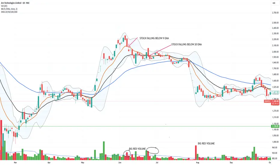
WHEN TO SELL A STOCKExit strategy is just as important as entry strategy.
We can use a daily close under the EMA's to sell our position.
We can trim 25% of our position in a stock when its price close under the 9 EMA.
We can avoid fake breakdown by closely monitoring the Volume.
Either a big Red Volume Candle (Increased Selling Interest) is an indication of upcoming fall in the Price movement.
We can trim 25% of our position in a stock when its price close under the 21 EMA.
Again have a close observation on the Volume candle to confirm the weakness.
Sell full position when the price of the stock fall below 50 EMA.
Note: The above chart is for educational purpose only.
Position Sizing for Different Trading Strategies1. Why Position Sizing Matters
Position sizing directly affects risk management. Even a profitable strategy can lead to account depletion if positions are too large relative to your capital. Conversely, if positions are too small, your returns will be suboptimal. Proper position sizing ensures that no single trade can jeopardize your entire trading account.
Key reasons position sizing matters:
Risk Control: Limits losses on any single trade.
Consistency: Ensures uniform risk exposure across trades.
Psychological Comfort: Helps traders manage emotions and stick to their strategy.
Maximizing Returns: Optimizes capital usage without taking excessive risk.
2. Core Concepts in Position Sizing
Before diving into strategy-specific sizing, understanding core concepts is essential:
2.1 Risk per Trade
This is the percentage of your total capital you are willing to risk on a single trade. Commonly, traders risk 1–3% per trade, depending on their risk tolerance.
2.2 Stop Loss
Stop loss defines the price at which you will exit a trade to prevent further losses. It directly influences position size: the closer the stop, the larger the position you can take, and vice versa.
2.3 Volatility
More volatile assets require smaller positions, as they are prone to larger price swings. Measures like Average True Range (ATR) help determine an appropriate position size relative to market volatility.
2.4 Account Size
Your total trading capital determines the absolute value of positions. Traders with smaller accounts may use tighter risk management rules to avoid blow-ups.
2.5 Reward-to-Risk Ratio
The potential reward compared to the risk taken affects sizing decisions. Higher reward-to-risk ratios may justify larger position sizes.
3. Position Sizing Methods
Several mathematical methods help determine the ideal position size:
3.1 Fixed Dollar Risk
You risk a fixed amount of money per trade regardless of the asset. For example, a trader risking $100 per trade will always limit losses to $100, whether trading a volatile stock or a low-volatility ETF.
3.2 Fixed Fractional
This method risks a fixed percentage of capital on each trade, which adjusts with account growth or decline. It is widely used due to its simplicity and adaptability.
Example:
With $50,000 capital and a 2% risk, the maximum loss per trade is $1,000. If the risk per share is $5, the position size is $1,000 ÷ $5 = 200 shares.
3.3 Volatility-Based Position Sizing
Adjusts position size according to market volatility. Higher volatility → smaller position size, lower volatility → larger position size. Tools like ATR are commonly used.
4. Position Sizing for Day Trading
Day traders enter and exit positions within the same day, often making multiple trades daily. Because trades are short-term and volatility can be high, risk management is crucial.
Typical Risk per Trade: 0.5–1% of account
Stop Loss: Tight, often based on intraday support/resistance or ATR
Position Size Method: Fixed fractional or volatility-based
Example:
If a trader has $100,000 and risks 1% ($1,000) per trade, with a $2 intraday stop, the position size is $1,000 ÷ $2 = 500 shares.
Key Tips for Day Traders:
Avoid over-leveraging during volatile sessions
Use intraday ATR for adjusting position size dynamically
Focus on liquidity to ensure smooth entry and exit
5. Position Sizing for Swing Trading
Swing traders hold positions from a few days to weeks to capture medium-term price moves. Risk is usually higher than day trading because positions are exposed to overnight and weekend gaps.
Typical Risk per Trade: 1–2% of account
Stop Loss: Wider than day trading, set based on technical levels
Position Size Method: Fixed fractional with ATR adjustment
Example:
A swing trader with $50,000 account risks 2% ($1,000). If the stop loss is $5 per share, the position size is 200 shares. For a stock with higher volatility (stop loss $10), the position size reduces to 100 shares.
Key Tips for Swing Traders:
Factor in overnight risk and earnings events
Adjust positions for volatility spikes
Diversify positions across sectors to reduce correlated risk
6. Position Sizing for Trend Following
Trend followers aim to ride long-term trends, often holding positions for weeks or months. These traders are willing to tolerate larger drawdowns in exchange for higher profits.
Typical Risk per Trade: 1–3%
Stop Loss: Wide, based on trend-defining support/resistance
Position Size Method: Volatility-based or fixed fractional with trailing stops
Example:
For a $100,000 account, a trend follower might risk 2% ($2,000) per trade. Using ATR for volatility measurement, a higher ATR reduces position size to prevent excessive risk during volatile trends.
Key Tips for Trend Followers:
Use volatility-adjusted stops to avoid getting stopped out prematurely
Scale into positions as trend strength confirms
Monitor correlation to avoid overexposure in the same market
7. Position Sizing for Scalping
Scalping involves making dozens or hundreds of trades per day to exploit small price movements. Risk per trade is tiny, but leverage and trade frequency increase overall risk.
Typical Risk per Trade: 0.1–0.25%
Stop Loss: Very tight, often a few ticks or cents
Position Size Method: Fixed fractional with tight risk controls
Example:
A scalper with $50,000 may risk 0.2% ($100) per trade. If stop loss is $0.10, the position size is $100 ÷ $0.10 = 1,000 shares/contracts.
Key Tips for Scalpers:
Execution speed and tight spreads are crucial
Monitor cumulative risk across multiple trades
Avoid trading during illiquid or volatile news events
8. Position Sizing for Options Trading
Options offer leverage, which makes position sizing critical. Option traders often risk a percentage of the premium or account rather than the underlying stock price.
Typical Risk per Trade: 1–3%
Stop Loss: Based on option premium or underlying price movement
Position Size Method: Fixed fractional or risk-defined based on delta
Example:
If a trader has $50,000 and risks 2% ($1,000) per trade on call options costing $5 each, they could buy 200 contracts.
Key Tips for Options Traders:
Factor in implied volatility changes
Avoid allocating too much capital to high-risk out-of-the-money options
Consider position delta to manage exposure to the underlying asset
9. Adjusting Position Size Based on Market Conditions
Market conditions influence position sizing significantly:
High Volatility: Reduce position size to limit risk
Low Volatility: Increase position size cautiously
Correlated Assets: Adjust sizes to prevent overexposure
Economic Events: Reduce exposure during major announcements
Dynamic position sizing is a hallmark of professional traders, allowing them to adapt to changing market environments without compromising risk control.
10. Common Mistakes in Position Sizing
Even experienced traders make mistakes with position sizing:
Ignoring Risk: Taking trades without defining risk can lead to catastrophic losses.
Overleveraging: Using excessive leverage magnifies small losses.
Inconsistent Sizing: Risking different percentages randomly undermines risk management.
Neglecting Volatility: Treating volatile assets the same as stable ones leads to oversized positions.
Not Scaling: Failing to adjust position size as account grows or shrinks.
Avoiding these mistakes is essential for long-term success.
11. Tools and Software for Position Sizing
Modern traders often rely on tools to calculate position size automatically:
Trading Platforms: MetaTrader, ThinkorSwim, NinjaTrader
Risk Calculators: Many online calculators allow inputs for account size, stop loss, and risk per trade
Excel Sheets: Customizable for advanced traders using multiple strategies
These tools save time and prevent errors in manual calculation.
12. Psychological Benefits of Proper Position Sizing
Position sizing is not only about numbers; it also affects trader psychology:
Confidence: Knowing risk is controlled reduces stress.
Discipline: Helps traders stick to strategy without emotional interference.
Consistency: Prevents revenge trading after losses.
A trader who masters position sizing often experiences steadier account growth and lower emotional volatility.
13. Summary and Best Practices
Position sizing is a cornerstone of risk management and long-term trading success. Key takeaways:
Determine your risk per trade relative to account size.
Adjust size based on stop loss, volatility, and trading strategy.
Use fixed fractional, volatility-based, or Kelly criterion methods.
Day traders use tight stops and small risks, swing traders use moderate risk and wider stops, trend followers rely on volatility-based sizing, and scalpers use very small per-trade risk.
Avoid common mistakes like ignoring volatility, overleveraging, or inconsistent sizing.
Employ tools and calculators to ensure accuracy.
Remember that position sizing protects both capital and mental composure.
By combining the right strategy with disciplined position sizing, traders can survive losses, ride profits, and grow their accounts consistently over time.
Conclusion:
Position sizing is the unsung hero of successful trading. It is what separates consistent traders from those who rely solely on prediction and luck. Whether you are a day trader, swing trader, trend follower, scalper, or options trader, understanding and applying proper position sizing can dramatically improve your risk-adjusted returns. Mastering this skill is not optional—it is essential for long-term profitability and trading survival.
Trading Strategies for MEME Stocks1. Understanding MEME Stocks
Before developing strategies, it’s essential to define what MEME stocks are:
Definition: MEME stocks are shares that gain popularity primarily through social media hype rather than traditional financial metrics. Examples include GameStop (GME), AMC Entertainment (AMC), and others.
Volatility: They are extremely volatile, often moving 20–50% in a single day based on social sentiment rather than earnings reports.
Market Influences: Retail investor activity, viral posts, and short squeezes heavily influence price movements.
Understanding these characteristics is the foundation for building effective trading strategies.
2. Core Principles of Trading MEME Stocks
Trading MEME stocks requires a different mindset than traditional investing. The following principles are critical:
Momentum Focus: MEME stocks move quickly, often with no correlation to fundamentals. Traders need to follow momentum rather than intrinsic value.
Sentiment Analysis: Monitoring social media trends, forum discussions, and news can provide insights into potential surges.
Risk Management: High volatility demands strict stop-loss levels to avoid catastrophic losses.
Quick Decision-Making: Entry and exit decisions must be executed rapidly as price swings can be extreme within hours.
These principles will guide strategy development.
3. Momentum Trading Strategy
Momentum trading is one of the most effective approaches for MEME stocks.
Steps:
Identify Trending Stocks: Use screeners or social platforms to identify stocks with surging discussions and trading volume.
Confirm Volume: High trading volume validates momentum. Sudden spikes in volume often precede price surges.
Technical Entry Points: Enter trades on breakouts above resistance levels or strong bullish candlestick patterns.
Exit Strategy: Exit on signs of weakening momentum or reversal patterns. Trailing stop-loss orders can protect profits while allowing for upside continuation.
Advantages:
Captures large price swings.
Utilizes short-term opportunities effectively.
Risks:
False breakouts can result in rapid losses.
Requires constant monitoring of market sentiment.
4. Social Media Sentiment Analysis
MEME stocks are uniquely sensitive to online sentiment. Traders can leverage this through:
Reddit Monitoring: Subreddits like WallStreetBets provide early signals of potential surges.
Twitter and Discord: Influential accounts and trending discussions can influence retail trading behavior.
News Aggregators: Platforms like Finviz or Stocktwits track viral news and chatter.
Implementation:
Track keywords and hashtags related to the stock.
Look for sudden spikes in mentions or engagement metrics.
Cross-reference sentiment with trading volume for confirmation.
Benefit:
Sentiment analysis allows traders to anticipate moves before they materialize in price charts, giving a first-mover advantage.
5. Short Squeeze Strategy
Short squeezes are a common driver of MEME stock rallies.
Understanding Short Squeezes:
A short squeeze occurs when heavily shorted stocks experience sudden buying pressure.
Short sellers are forced to cover positions, driving prices higher rapidly.
Strategy Steps:
Identify Heavily Shorted Stocks: Use short interest ratios and data from platforms like FINRA.
Monitor Trigger Events: Positive news, social media hype, or momentum indicators can trigger a squeeze.
Entry Point: Enter during early signs of short covering, often indicated by rising volume and sudden price jumps.
Exit Point: Take profits as soon as momentum shows signs of fading or when price becomes unsustainably high.
Advantages:
Can generate rapid gains in short periods.
High potential ROI if timed correctly.
Risks:
Extremely volatile; timing is critical.
Losses can be significant if squeeze fails.
6. Technical Analysis for MEME Stocks
While fundamentals may take a backseat, technical analysis is crucial for MEME trading.
Key Tools:
Support and Resistance Levels: Identify critical price levels for entry and exit.
Moving Averages: Short-term moving averages (e.g., 5-day, 20-day) help identify momentum trends.
Relative Strength Index (RSI): Helps spot overbought or oversold conditions, useful in predicting reversals.
Candlestick Patterns: Patterns like bullish engulfing, hammers, or doji can signal potential reversals or continuation.
Best Practices:
Combine multiple indicators for confirmation.
Focus on intraday and short-term charts (1-min, 5-min, 15-min) for trade timing.
Avoid relying solely on a single technical signal due to high volatility.
7. Risk Management Strategies
Risk management is arguably the most critical aspect of MEME stock trading.
Techniques:
Position Sizing: Never allocate more than a small percentage of capital to a single trade (e.g., 1–5%).
Stop-Loss Orders: Protect against sharp reversals by placing stop-loss orders slightly below support levels.
Take-Profit Levels: Predefine exit points to lock in gains amid rapid volatility.
Diversification: Spread investments across multiple MEME stocks to reduce exposure to a single trend.
Psychology:
Emotional discipline is key. MEME stocks can be highly addictive due to rapid gains.
Avoid chasing price spikes; stick to pre-defined trade plans.
8. Swing Trading Strategy
Swing trading is suitable for traders looking to hold MEME stocks for several days or weeks.
Steps:
Identify Trend: Use daily or weekly charts to find uptrending MEME stocks.
Entry Point: Buy during temporary pullbacks in an overall uptrend.
Exit Point: Sell near resistance levels or when technical indicators show momentum fading.
Monitoring: Keep track of news, social sentiment, and earnings reports as catalysts for continued momentum.
Benefits:
Captures larger trends than intraday trades.
Less stressful than constant intraday monitoring.
Risks:
Overnight gaps can result in unexpected losses.
Requires patience and confidence in trend continuation.
9. Scalping Strategy
For highly active traders, scalping offers opportunities to profit from intraday volatility.
Methodology:
Use Short Timeframes: Focus on 1-minute or 5-minute charts.
Frequent Trades: Execute multiple small trades targeting minor price fluctuations.
Technical Indicators: Leverage moving averages, Bollinger Bands, and volume indicators.
Quick Exit: Close positions as soon as targets are met, avoiding large drawdowns.
Advantages:
Takes advantage of rapid price movements typical in MEME stocks.
Reduces exposure to overnight risk.
Risks:
Demands full attention and fast execution.
High transaction costs may eat into profits.
10. Psychological and Behavioral Considerations
Trading MEME stocks is as much a psychological game as a technical one.
Herd Mentality: Many traders follow the crowd, creating self-fulfilling price spikes.
Fear of Missing Out (FOMO): Can lead to impulsive entries at peak prices.
Patience and Discipline: Successful traders avoid emotional decision-making and stick to predefined strategies.
Avoiding Overexposure: MEME stocks can dominate media headlines, but not all hype translates into sustainable profits.
Understanding these behavioral aspects is crucial for surviving the extreme volatility inherent in MEME stocks.
11. Tools and Platforms for MEME Stock Trading
Traders can leverage various tools to improve their decision-making:
Trading Platforms: Robinhood, Webull, Zerodha, and Interactive Brokers offer easy access to MEME stocks.
Screeners: Tools like Finviz, TradingView, and Yahoo Finance help identify trending stocks.
Social Media Analytics: Platforms like Stocktwits, Reddit tracking tools, and Twitter analytics assist in sentiment monitoring.
Technical Indicators: TradingView and MetaTrader allow charting with customizable indicators for intraday and swing trading strategies.
12. Common Mistakes to Avoid
Ignoring Risk Management: Overleveraging can lead to catastrophic losses.
Chasing Hype: Entering trades at peak prices often results in losses when momentum fades.
Neglecting Exit Strategy: MEME stocks can reverse quickly; predefined exit points are essential.
Overtrading: Excessive trading increases costs and emotional stress.
Avoiding these pitfalls can improve long-term success.
13. Conclusion
Trading MEME stocks is an exhilarating but highly risky endeavor. Unlike traditional investing, it relies heavily on momentum, social sentiment, and short-term price action rather than fundamental valuation. Successful MEME traders combine multiple strategies:
Momentum and swing trading for capturing trends.
Sentiment analysis to anticipate moves.
Short squeeze exploitation for rapid gains.
Strict risk management to safeguard capital.
Additionally, psychological discipline and adherence to predefined trading rules are critical. While MEME stocks can generate extraordinary returns, they demand careful planning, continuous monitoring, and a clear understanding of the volatile forces at play. By applying these strategies thoughtfully, traders can navigate the exciting world of MEME stocks while mitigating the risks inherent in this unconventional market segment.
Outlook Cycles and the Importance of Cycle Analysis in TradingIntroduction to Outlook Cycles
Trading in financial markets is as much an art as it is a science. Among the tools that experienced traders use to anticipate market movements, outlook cycles play a critical role. An outlook cycle refers to the recurring patterns or phases in the market that repeat over time. These cycles are not arbitrary; they emerge from the collective psychology of market participants, macroeconomic trends, corporate earnings patterns, and broader financial and geopolitical influences.
Understanding these cycles allows traders to anticipate potential market turning points and adjust their strategies accordingly. While cycles do not guarantee exact price movements, they provide a probabilistic framework for predicting trends and reversals, making them invaluable for strategic planning in trading.
Defining Outlook Cycles
An outlook cycle in trading can be described as a repetitive sequence of market behavior, typically measured in time units such as days, weeks, months, or even years. These cycles can manifest across various financial instruments including stocks, commodities, currencies, and indices.
Key Features of Outlook Cycles
Repetition: Patterns tend to recur in similar forms over time.
Predictability: While not exact, they provide insight into probable future movements.
Duration: Cycles can be short-term (intra-day to weekly) or long-term (monthly, quarterly, yearly).
Amplitude: Cycles vary in magnitude, influencing how strongly price moves during different phases.
Types of Outlook Cycles
Outlook cycles can be categorized based on their duration and underlying factors:
Short-term cycles:
Usually last from a few hours to a few weeks.
Influenced by market sentiment, news, technical setups, and trader behavior.
Example: Stock price oscillations around support and resistance levels.
Intermediate cycles:
Typically span several weeks to months.
Influenced by quarterly earnings, monetary policy announcements, and macroeconomic indicators.
Example: Seasonal patterns in commodities or consumer stocks during festive periods.
Long-term cycles:
Extend from several months to multiple years.
Driven by fundamental shifts such as economic expansions or recessions, geopolitical events, or major technological disruptions.
Example: Bull and bear market cycles in equities or long-term commodity demand cycles.
Importance of Cycle Analysis in Trading
Cycle analysis is a crucial aspect of trading because it enables traders to anticipate market movements rather than react to them. Here are the key reasons why cycle analysis is vital:
1. Identifying Market Phases
Every market moves in phases: accumulation, uptrend, distribution, and downtrend.
Accumulation Phase: In this phase, smart money often accumulates positions quietly. Price moves are subtle but set the stage for the next upward move.
Uptrend Phase: Characterized by increasing prices, often driven by retail participation and positive sentiment.
Distribution Phase: Large investors start taking profits, leading to sideways or slightly downward movement.
Downtrend Phase: Prices decline as panic selling and negative sentiment dominate.
Cycle analysis helps traders identify these phases in advance, providing an edge in entering or exiting trades.
2. Timing Entries and Exits
By studying cycles, traders can refine their entry and exit points, rather than relying solely on price action or technical indicators. For instance:
Buying near the beginning of an uptrend cycle maximizes profit potential.
Selling or shorting near the peak of a cycle helps avoid losses during downturns.
This timing advantage is particularly critical in volatile markets where even a few days of misjudgment can result in significant losses.
3. Managing Risk
Cycle analysis allows traders to implement risk management strategies based on the stage of the market cycle. For example:
During a downward cycle, traders may reduce position size or hedge portfolios using options or inverse ETFs.
During upward cycles, traders may take on higher risk positions to capitalize on strong trends.
Understanding cycles provides a risk-reward framework rather than trading blindly.
4. Enhancing Strategy Development
Traders often combine cycle analysis with other methods like technical indicators, fundamentals, and sentiment analysis to create robust trading strategies.
Example: Using moving averages or Fibonacci retracements in conjunction with cycle peaks and troughs can improve accuracy.
Example: Combining economic data releases with known seasonal cycles in commodities (like oil or agricultural products) enhances decision-making.
5. Psychological Advantage
Markets are driven by human behavior, which is inherently cyclical. Fear, greed, optimism, and panic repeat across generations of investors. By recognizing these recurring emotional patterns, traders gain a psychological advantage over the average participant who trades impulsively.
6. Recognizing External Influences
Outlook cycles also help traders understand how external factors influence markets, such as:
Central bank policies affecting interest rates and liquidity.
Geopolitical tensions causing volatility in commodities like oil and gold.
Seasonal economic trends, such as holiday shopping periods boosting retail stocks.
By correlating cycles with external events, traders can anticipate market reactions rather than merely respond after the fact.
Practical Applications of Cycle Analysis
Stock Market Trading:
Identifying earnings cycles, dividend announcements, and market sentiment peaks.
Recognizing seasonal patterns, e.g., “Sell in May and go away” trend in equities.
Forex Trading:
Analyzing interest rate cycles, central bank policy cycles, and currency correlations.
Predicting trends based on geopolitical events affecting specific currencies.
Commodity Trading:
Tracking seasonal demand-supply cycles, such as oil demand in summer or agricultural harvesting cycles.
Understanding macroeconomic cycles like inflationary pressures influencing precious metals.
Options and Derivatives Trading:
Identifying implied volatility cycles to time option purchases or sales.
Understanding cyclical patterns in futures markets for hedging and speculative purposes.
Tools for Cycle Analysis
Several tools and techniques help traders analyze market cycles:
Technical Indicators:
Moving Averages, MACD, RSI, and Stochastic oscillators can identify cyclical peaks and troughs.
Elliott Wave Theory:
Recognizes repeating patterns in market psychology and price action.
Useful in identifying primary, intermediate, and minor cycles.
Fourier and Spectral Analysis:
Advanced methods that break down price data into component cycles to detect periodicity.
Seasonal Charts and Historical Analysis:
Compare current market conditions with historical trends to anticipate recurring patterns.
Economic Calendars and Fundamental Analysis:
Aligning macroeconomic cycles with market cycles enhances predictive accuracy.
Challenges in Cycle Analysis
While outlook cycles provide significant insight, traders must be aware of certain limitations:
No Guarantee of Accuracy:
Cycles indicate probability, not certainty. External shocks can disrupt patterns unexpectedly.
Multiple Overlapping Cycles:
Short-term, intermediate, and long-term cycles can interact, sometimes creating conflicting signals.
Complex Interpretation:
Reading cycles requires experience and often involves combining multiple analytical techniques.
Dynamic Market Conditions:
Cycles can shift over time due to changes in market structure, regulations, or participant behavior.
Despite these challenges, skilled traders view cycles as guiding tools, not absolute rules.
Conclusion
Outlook cycles are a cornerstone of informed trading, offering a structured approach to understanding market dynamics. By analyzing cyclical patterns, traders can anticipate market phases, time entries and exits, manage risk, and gain a psychological edge. Whether in stocks, commodities, forex, or derivatives, cycle analysis complements technical and fundamental methods, creating a more holistic and strategic trading approach.
While cycles are not infallible, they provide a probabilistic framework for decision-making in uncertain markets. Traders who master cycle analysis can move from reactive trading to proactive, calculated strategies, enhancing their potential for consistent profitability.
In short, understanding outlook cycles transforms market uncertainty into strategic opportunity, making cycle analysis one of the most valuable tools in a trader’s toolkit.

What Makes Crypto Different from Traditional AssetsIntroduction
Cryptocurrencies have emerged over the last decade as a revolutionary form of digital asset, capturing global attention for their potential to redefine finance, investment, and even societal trust. Unlike traditional assets such as stocks, bonds, and fiat currencies, crypto operates on decentralized networks and utilizes cryptographic principles. While traditional assets have been the cornerstone of financial markets for centuries, crypto introduces novel features and risks that set it apart. Understanding these differences is crucial for investors, policymakers, and anyone interested in the evolution of financial markets.
1. Nature of the Asset
Traditional Assets: Traditional financial assets represent ownership in a tangible or legal entity. For example, stocks signify a share of ownership in a company, bonds are debt instruments promising future repayment, and real estate represents physical property. Their value is often tied to cash flows, earnings, or physical utility.
Cryptocurrencies: Cryptocurrencies are purely digital assets, existing only on a blockchain—a distributed ledger maintained by a network of computers. They do not inherently represent ownership of a company or tangible goods (except for certain tokenized assets). Their value derives from scarcity (like Bitcoin’s capped supply), network adoption, and market sentiment rather than conventional cash flows.
Key Difference: Crypto is an intangible, digital-only asset whose value is largely determined by market perception, adoption, and underlying blockchain technology, unlike traditional assets which are tied to tangible ownership or income streams.
2. Decentralization and Control
Traditional Assets: Traditional assets are regulated and controlled by central authorities such as governments, central banks, and regulatory bodies. For instance, stock markets operate under oversight from institutions like the SEC in the United States. Transactions are intermediated by banks, brokers, and clearinghouses, ensuring compliance with legal frameworks.
Cryptocurrencies: Most cryptocurrencies operate on decentralized networks, meaning no single entity controls the system. Transactions are verified by a distributed network of nodes using consensus mechanisms such as proof-of-work or proof-of-stake. Users can transact peer-to-peer without intermediaries, reducing reliance on centralized authorities.
Key Difference: Crypto offers decentralization and autonomy, whereas traditional assets rely heavily on centralized intermediaries for governance and transaction verification.
3. Supply and Inflation Mechanisms
Traditional Assets: Fiat currencies are subject to monetary policy, with central banks controlling supply to influence inflation, interest rates, and economic growth. Stocks are issued at the discretion of companies, and bonds follow government or corporate debt issuance schedules. The supply can be increased or adjusted according to policy or corporate strategy.
Cryptocurrencies: Cryptos like Bitcoin have fixed supplies encoded in their protocols (Bitcoin’s maximum supply is 21 million coins). Other cryptocurrencies use algorithms to control issuance and incentivize network participation. This scarcity is designed to emulate deflationary characteristics, contrasting with the often inflationary nature of fiat currencies.
Key Difference: Crypto supply is usually pre-determined and algorithmically enforced, whereas traditional assets are subject to discretionary management and central control.
4. Liquidity and Market Accessibility
Traditional Assets: Stocks and bonds are traded on regulated exchanges with established liquidity and market hours. Investors often require brokerage accounts, and trading may be limited by jurisdictional regulations. While liquidity is generally high for large-cap assets, small markets may suffer from limited participants.
Cryptocurrencies: Crypto markets operate 24/7 globally with virtually no geographic restrictions. Anyone with internet access can buy, sell, or hold crypto, often without the need for traditional intermediaries. However, liquidity can vary widely between coins; while Bitcoin and Ethereum are highly liquid, smaller tokens may be subject to high volatility and thin markets.
Key Difference: Crypto markets are continuously accessible and globally decentralized, unlike traditional markets with operational hours and regional constraints.
5. Volatility and Risk Profile
Traditional Assets: Traditional assets tend to have established risk-return profiles. While stocks can be volatile, especially in emerging sectors, they are generally less erratic compared to crypto. Bonds provide predictable returns with lower volatility, and commodities fluctuate based on supply-demand fundamentals.
Cryptocurrencies: Cryptos are highly volatile. Prices can swing 10–20% in a single day due to market sentiment, regulatory news, or technical developments. While volatility offers opportunities for high returns, it also carries substantial risk. Crypto markets are less mature and less predictable than traditional markets.
Key Difference: Crypto’s extreme volatility distinguishes it as a high-risk, high-reward asset class, unlike the relatively stable behavior of traditional financial assets.
6. Regulation and Legal Framework
Traditional Assets: Traditional financial assets operate under well-established legal frameworks and are protected by investor safeguards. Securities laws, accounting standards, and regulatory oversight aim to reduce fraud and systemic risk.
Cryptocurrencies: Crypto regulation is still evolving. Some countries have embraced it, creating frameworks for trading, taxation, and custody, while others ban or restrict usage. Lack of regulation can lead to fraud, hacking, and market manipulation. Investor protections are often minimal compared to traditional markets.
Key Difference: Traditional assets are highly regulated with legal recourse for investors, whereas crypto operates in a more ambiguous and evolving regulatory environment.
7. Transparency and Verification
Traditional Assets: Transparency in traditional assets is often limited to financial reporting, audits, and regulatory filings. Verification of ownership or transactions usually requires intermediaries like banks or clearinghouses.
Cryptocurrencies: Blockchains provide public, immutable ledgers where anyone can verify transactions without intermediaries. Smart contracts enable automatic execution of agreements. This transparency reduces the need for trust in centralized authorities but requires understanding of blockchain technology.
Key Difference: Crypto enables direct, verifiable transparency of transactions, while traditional assets rely on intermediaries for reporting and verification.
8. Divisibility and Portability
Traditional Assets: While fiat currencies are divisible and easily transferable, assets like real estate or certain bonds are not easily fractioned or transferred. Stocks can be subdivided through shares, but some physical assets remain illiquid or cumbersome.
Cryptocurrencies: Cryptos are highly divisible; for example, Bitcoin can be split into 100 million units called satoshis. Digital nature makes them extremely portable and transferrable across borders instantly with minimal fees compared to traditional banking systems.
Key Difference: Cryptos offer unmatched divisibility and portability, enhancing flexibility for small and large investors alike.
9. Innovation and Utility
Traditional Assets: The utility of traditional assets is relatively straightforward—stocks provide ownership, bonds offer interest, and commodities have industrial or consumption uses. Innovation in traditional finance occurs, but structural changes are slow due to regulatory and institutional constraints.
Cryptocurrencies: Cryptos are more than just assets; they enable decentralized finance (DeFi), tokenization, programmable money, and novel applications like NFTs. They offer utility within their ecosystems, such as participating in governance, staking, and decentralized applications.
Key Difference: Cryptos combine financial value with technological utility, whereas traditional assets primarily serve as stores of value or income generation tools.
10. Security and Custody
Traditional Assets: Security in traditional finance depends on trusted intermediaries—banks, brokers, and clearinghouses. Physical assets can be insured, and digital assets in broker accounts are protected by legal frameworks.
Cryptocurrencies: Crypto security is decentralized but relies heavily on private key management. Loss of keys can mean permanent loss of funds. While blockchain is secure by design, exchanges and wallets have been hacked, emphasizing the importance of personal custody practices.
Key Difference: Crypto security shifts responsibility to the individual, unlike traditional assets where intermediaries shoulder the protection burden.
11. Global Accessibility and Inclusivity
Traditional Assets: Access to traditional assets often requires citizenship, residency, or local bank accounts. Emerging markets may face barriers due to infrastructure limitations or regulatory constraints.
Cryptocurrencies: Crypto allows anyone with internet access to participate in global markets. It can provide financial inclusion to unbanked populations, bypassing traditional barriers.
Key Difference: Cryptos are inherently borderless and democratizing, while traditional assets are constrained by geography and regulatory frameworks.
Conclusion
Cryptocurrencies fundamentally differ from traditional assets across multiple dimensions: nature, control, supply mechanisms, liquidity, risk, regulation, transparency, divisibility, innovation, security, and accessibility. Traditional assets are backed by tangible entities or cash flows, regulated by authorities, and generally stable, while crypto thrives on decentralization, digital scarcity, and technological innovation.
These differences create opportunities and challenges. On one hand, crypto democratizes finance, allows for 24/7 global markets, and enables programmable financial tools. On the other hand, it introduces high volatility, regulatory uncertainty, and security risks. As the financial landscape evolves, understanding these distinctions is critical for investors, regulators, and innovators aiming to navigate both traditional and digital asset ecosystems.
Cryptocurrency is not merely an alternative investment; it represents a paradigm shift in how value, trust, and financial transactions are conceived. While traditional assets remain foundational to wealth creation, crypto pushes the boundaries of what constitutes money, ownership, and economic participation in the 21st century.
Policy Developments in Derivatives and Commodities MarketsIntroduction
The derivatives and commodities markets are critical components of the global financial system. They provide essential tools for risk management, price discovery, and investment diversification. Derivatives—contracts whose value derives from underlying assets like commodities, equities, or currencies—enable participants to hedge against price volatility. Commodities markets, on the other hand, facilitate trading in raw materials such as oil, metals, and agricultural products.
Over the past few decades, these markets have witnessed significant evolution in both their structure and regulatory frameworks. Policymakers and regulatory authorities across the globe have introduced reforms to enhance transparency, reduce systemic risk, and promote market efficiency. These policy developments have become increasingly important in light of financial crises, technological advancements, globalization of markets, and growing participation from retail investors.
1. Historical Context of Derivatives and Commodities Regulation
The regulation of derivatives and commodities markets has evolved in response to market crises and structural changes. Historically, commodities trading, especially in agricultural products, was lightly regulated, primarily aimed at preventing fraud and market manipulation. In contrast, modern derivative markets grew exponentially in the 1980s and 1990s with the rise of financial engineering and complex instruments like options, swaps, and futures.
Major events that shaped policy include:
The 1987 Stock Market Crash: Highlighted the need for robust oversight of derivative instruments and their impact on financial markets.
The 2008 Global Financial Crisis: Exposed systemic risks inherent in over-the-counter (OTC) derivatives markets, prompting regulators to focus on transparency, collateralization, and centralized clearing mechanisms.
Commodity Price Volatility: Sharp swings in oil, metals, and agricultural products prices led to government interventions to stabilize markets, protect consumers, and ensure fair trading practices.
These events underscored the importance of developing robust regulatory frameworks to safeguard market integrity while fostering innovation.
2. Objectives of Policy Developments
Regulatory policies in derivatives and commodities markets aim to achieve several key objectives:
Market Integrity: Preventing manipulation, insider trading, and fraudulent practices.
Transparency: Ensuring that market participants have access to accurate and timely information about prices, trading volumes, and open positions.
Financial Stability: Reducing systemic risk that arises from excessive leverage, interconnected financial institutions, and OTC derivatives exposures.
Consumer Protection: Safeguarding investors, particularly retail participants, from misleading practices or excessive risk exposure.
Promotion of Market Efficiency: Ensuring smooth price discovery and liquidity in the markets.
Alignment with International Standards: Harmonizing domestic regulations with global best practices set by organizations such as the International Organization of Securities Commissions (IOSCO) and the Financial Stability Board (FSB).
3. Key Policy Developments in Derivatives Markets
3.1 Introduction of Central Clearing
One of the most significant reforms after the 2008 financial crisis was the push for central clearing of standardized OTC derivatives. Central counterparties (CCPs) act as intermediaries between buyers and sellers, reducing counterparty risk. Regulatory frameworks such as Dodd-Frank Act (USA, 2010) and the European Market Infrastructure Regulation (EMIR, EU, 2012) mandated clearing of certain interest rate and credit derivatives through CCPs.
Impact:
Reduced systemic risk from bilateral exposures.
Standardized collateral requirements.
Improved market transparency.
3.2 Trade Reporting and Transparency
Regulators worldwide have introduced mandatory trade reporting requirements to enhance transparency in derivatives markets. Trade repositories collect and publish data on derivative transactions, including notional amounts, counterparties, and trade dates.
Examples of regulatory measures:
Dodd-Frank Act: Requires real-time reporting of swaps transactions to swap data repositories.
EMIR: Obligates EU market participants to report derivative trades to trade repositories.
Impact:
Increased market visibility.
Facilitated monitoring of systemic risk and market abuse.
3.3 Margin and Collateral Requirements
To mitigate counterparty risk, regulators have introduced margin requirements for both cleared and non-cleared derivatives. Initial margin protects against potential default losses, while variation margin ensures that daily gains and losses are settled.
Impact:
Reduced excessive leverage in derivatives trading.
Promoted financial stability and investor confidence.
3.4 Standardization of Contracts
Policy frameworks encourage the standardization of derivative contracts to facilitate central clearing and improve liquidity. Standardization covers contract size, settlement dates, underlying asset definitions, and documentation standards.
Impact:
Easier to trade on exchanges or through CCPs.
Lower operational and legal risks for participants.
3.5 Risk-Based Supervision
Regulators are increasingly adopting risk-based approaches to monitor derivative markets. This involves focusing on systemically important institutions, products, and trading strategies that could pose the greatest risk to financial stability.
Impact:
Efficient use of regulatory resources.
Early identification and mitigation of systemic threats.
4. Key Policy Developments in Commodities Markets
4.1 Position Limits and Speculation Controls
Excessive speculative trading can destabilize commodity prices. Regulators have introduced position limits to restrict the number of contracts a participant can hold in futures markets. These limits aim to prevent market manipulation and excessive concentration of risk.
Examples:
Commodity Futures Trading Commission (CFTC) in the US sets speculative position limits for energy, metals, and agricultural contracts.
Securities and Exchange Board of India (SEBI) imposes position limits in commodity futures markets to curb volatility.
4.2 Market Surveillance and Anti-Manipulation Measures
Commodity exchanges and regulators have strengthened market surveillance to detect and prevent price manipulation, spoofing, and front-running. Sophisticated monitoring systems track trading patterns in real-time to identify anomalies.
Impact:
Enhanced investor confidence.
Reduced market distortions caused by artificial price movements.
4.3 Integration with Global Markets
Globalization of commodities trading has prompted harmonization of regulations across borders. Policymakers focus on aligning rules regarding contract specifications, reporting, and settlement to facilitate international participation.
Examples:
Cross-border recognition of clearinghouses.
Adoption of international standards on warehouse receipts and quality certification for agricultural commodities.
4.4 Commodity Derivatives for Hedging and Risk Management
Governments encourage the use of commodity derivatives for legitimate hedging purposes by producers, consumers, and traders. Policy initiatives include reducing regulatory burdens for hedgers while monitoring speculative activities.
Impact:
Enhanced price discovery and risk management.
Support for farmers, manufacturers, and energy companies in managing input costs.
4.5 Technological Innovations and Policy Adaptation
Digital trading platforms, algorithmic trading, and blockchain-based commodity exchanges have transformed the market landscape. Regulators are adapting policies to address new risks, including cyber threats, algorithmic market manipulation, and transparency challenges in decentralized trading.
Impact:
Improved market efficiency and accessibility.
Necessitated development of technology-driven monitoring tools.
5. Emerging Trends in Policy Development
Sustainability and ESG Integration: Policies increasingly emphasize environmental, social, and governance (ESG) compliance. Commodity trading in carbon credits, renewable energy certificates, and ESG-linked derivatives is growing.
Retail Participation Regulation: With growing retail interest in commodities and derivatives, regulators are introducing education initiatives, leverage limits, and product suitability requirements.
Cross-Market Risk Management: Integrated policies are addressing interconnected risks between derivatives, commodities, and other financial markets.
Global Coordination: Bodies like the IOSCO and FSB coordinate policy frameworks to prevent regulatory arbitrage and systemic instability.
6. Challenges in Policy Implementation
Despite significant reforms, regulators face several challenges:
Complexity of Derivative Products: Highly customized contracts are difficult to monitor and standardize.
Global Market Fragmentation: Different jurisdictions have varied regulatory standards, creating arbitrage opportunities.
Technological Disruptions: High-frequency trading, AI-based strategies, and decentralized exchanges introduce new risks.
Balancing Innovation and Risk: Policymakers must ensure that innovation is not stifled while protecting market participants.
7. Conclusion
Policy developments in derivatives and commodities markets have transformed these markets into safer, more transparent, and efficient mechanisms for risk management and investment. Central clearing, trade reporting, margin requirements, and position limits have enhanced market integrity and financial stability. Regulatory emphasis on transparency, standardization, and risk-based supervision has reduced systemic threats while fostering investor confidence.
As these markets continue to evolve with globalization, technological innovation, and ESG integration, policymakers must remain agile. Future regulatory frameworks are likely to focus on harmonizing global standards, enhancing surveillance capabilities, promoting sustainability, and safeguarding retail participants. Effective policy development in derivatives and commodities markets not only mitigates risks but also ensures that these markets continue to serve as vital tools for price discovery, hedging, and economic growth.
Understanding ‘Trade the Headline’: What It Really Means1. The Basics: What is ‘Trade the Headline’?
At its core, trading the headline means making market decisions based on breaking news or scheduled economic announcements. These headlines can range from interest rate decisions by central banks to employment reports, geopolitical events, corporate earnings, or even unexpected crises.
Traders aim to capitalize on the market reaction to these events rather than relying solely on charts or technical indicators. Essentially, the strategy assumes that the headline will trigger volatility, which can then be exploited for profit.
For example, if a central bank announces an unexpected interest rate cut, traders might buy the currency to take advantage of its immediate appreciation. Conversely, bad earnings news might prompt a trader to short a stock.
2. Why Headlines Move Markets
Financial markets are fundamentally influenced by information. Price is a reflection of what participants collectively believe about the future value of an asset. A headline can shift that belief instantly.
Some key reasons headlines move markets:
New Information: Markets react to information that changes expectations. A positive jobs report can boost a currency because it signals economic strength.
Surprise Factor: It’s not just the news itself but how it differs from expectations. A forecasted GDP growth of 3% vs. an actual 4% can cause a surge in market activity.
Liquidity and Herd Behavior: Headlines often trigger stop orders, algorithmic trading, and herd behavior, amplifying price movements.
Emotional Response: Traders’ sentiment—fear, greed, and uncertainty—can exaggerate reactions to news.
3. Types of Headlines That Matter
Not all headlines have equal impact. Traders focus on those that are market-moving:
Economic Data: Inflation reports, unemployment numbers, retail sales, PMI, and GDP announcements.
Central Bank Decisions: Interest rates, monetary policy statements, and quantitative easing programs.
Corporate Earnings: Quarterly earnings surprises, guidance updates, and mergers/acquisitions.
Geopolitical Events: Wars, elections, trade agreements, sanctions, or political instability.
Unexpected Shocks: Natural disasters, pandemics, or major cyberattacks.
The significance often depends on timing, market expectations, and the affected asset class. For instance, forex traders are highly sensitive to interest rate decisions, whereas equity traders may focus more on earnings reports.
4. The Mechanics of Trading the Headline
Trading the headline involves several steps:
Step 1: Preparation
Traders identify the news events that are likely to influence their markets.
Economic calendars and news feeds are essential tools.
They also note the consensus expectations, because market reactions often hinge on surprises rather than the raw data.
Step 2: Anticipation
Traders decide whether to enter before the news or wait for confirmation after the market reacts.
Pre-news positioning is riskier because if the headline differs from expectations, positions can move against the trader sharply.
Waiting for confirmation reduces risk but might limit profit opportunities.
Step 3: Execution
Traders enter positions based on expected or confirmed reactions.
Rapid execution is crucial as news-driven moves can occur within seconds.
Techniques often include stop orders, limit orders, or algorithmic trading.
Step 4: Risk Management
Volatility around headlines is unpredictable; stops can be triggered by temporary spikes.
Traders often reduce position size and use tight stop-losses to manage risk.
Some even avoid trading headlines altogether due to extreme unpredictability.
5. Strategies for Trading the Headline
Several strategies exist:
a. Pre-Announcement Positioning
Traders take positions before the news based on predictions.
Advantage: High potential profits if the market moves as anticipated.
Disadvantage: High risk if the news surprises in the opposite direction.
b. Reactionary Trading
Traders wait for the market to react to the headline before entering.
Advantage: Reduced risk of being caught on the wrong side of a surprise.
Disadvantage: Smaller profits as initial moves may be captured by faster traders or algorithms.
c. Fade the Move
Traders go against the initial market reaction, anticipating that the move will reverse.
Often used when headlines produce overreactions.
Requires experience and discipline.
d. Volatility-Based Options Trading
In options markets, traders might buy straddles or strangles to profit from expected volatility, regardless of direction.
This approach is common around central bank announcements or earnings reports.
6. The Psychology Behind Trading the Headline
The ability to trade headlines successfully is not just technical—it’s psychological:
Fear and Greed: Breaking news can trigger panic buying or selling, creating rapid price swings.
Herd Mentality: Traders often mimic the crowd, amplifying volatility.
Decision-Making Under Pressure: News trading requires split-second decisions, which can be stressful and emotionally taxing.
Confirmation Bias: Traders may interpret headlines to fit pre-existing beliefs, leading to mistakes.
Managing these psychological factors is crucial for consistent success.
7. Risks of Trading the Headline
While the potential for quick profits is high, so is the risk:
Whipsaw Movements: Prices may spike and reverse quickly, hitting stops and causing losses.
Low Liquidity Spikes: Some events can create temporary illiquidity, widening spreads and increasing slippage.
Algorithmic Dominance: High-frequency trading algorithms often react faster than human traders.
Unexpected Surprises: Even well-predicted news can cause moves in the opposite direction if the market interprets it differently.
Emotional Stress: Constant monitoring of news and fast execution can lead to burnout.
8. Tools and Techniques for Trading Headlines
Successful news traders rely on several tools:
Economic Calendars: Sites like Forex Factory, Investing.com, and Bloomberg provide upcoming event schedules and consensus forecasts.
News Feeds: Real-time feeds from Reuters, Bloomberg, or Dow Jones allow immediate access to breaking headlines.
Charting Platforms: Help track reactions in real-time and place quick orders.
Algorithmic Tools: Many traders use bots or scripts to automate reactions to specific news events.
Volatility Indicators: Metrics like ATR (Average True Range) can help adjust position sizing during high-volatility periods.
9. Real-World Examples
Central Bank Interest Rate Decisions
When the Federal Reserve announces unexpected rate hikes, the USD can spike within seconds.
Traders who anticipated the move may profit, while those caught off-guard can suffer losses.
Employment Reports
U.S. Non-Farm Payroll (NFP) data often triggers large forex moves.
Traders watch the actual number versus expectations, with discrepancies causing volatility.
Corporate Earnings Surprises
A tech company exceeding revenue expectations can see its stock soar, while a miss can trigger a sell-off.
Short-term traders capitalize on these price swings.
10. Best Practices for Trading the Headline
Do Your Homework: Know the key events and consensus expectations.
Use Risk Management: Set stop-losses and manage position sizes carefully.
Avoid Emotional Trading: Stick to a plan and avoid chasing the market.
Focus on Major Moves: Not every headline is worth trading; focus on high-impact events.
Have a Contingency Plan: Be prepared for unexpected spikes, illiquidity, or slippage.
11. Conclusion
“Trade the headline” is more than just reacting to news. It is a strategic approach that requires preparation, timing, and discipline. While the potential for rapid profits exists, so do substantial risks. Success depends on understanding market expectations, human psychology, and volatility dynamics, as well as employing strict risk management.
For traders, trading the headline can be exciting and profitable, but it is not a casual endeavor. It demands a blend of analytical skill, quick decision-making, and emotional resilience. Those who master it can harness the power of information-driven market moves to gain an edge, while those who underestimate it risk being swept away by the very volatility they seek to exploit.
The Challenge of Growing a Small Trading Account1. Understanding the Limitations of a Small Account
The first challenge of growing a small trading account is understanding its inherent limitations. A small account, often ranging from a few hundred to a few thousand dollars, restricts the trader's ability to diversify and take large positions. Limited capital means that even minor mistakes can significantly affect overall performance.
Position Sizing: Small accounts require smaller trade sizes to avoid devastating losses. However, this also limits profit potential because even successful trades generate modest returns.
Diversification Constraints: With limited funds, traders cannot spread capital across multiple assets or markets, increasing vulnerability to single trade losses.
Leverage Risks: Many traders turn to leverage to amplify gains, but higher leverage dramatically increases the risk of margin calls and complete account wipeouts.
2. Psychological Pressures of Small Account Trading
Trading with a small account exerts intense psychological pressure. The fear of losing even a small percentage of capital can lead to hesitation or impulsive decision-making. Traders often experience emotional swings that impact their judgment:
Overtrading: Small accounts may push traders to take excessive trades to achieve significant returns, often leading to mistakes.
Fear and Anxiety: Losing a small portion of a tiny account feels proportionally larger, which can magnify fear and trigger panic selling.
Greed: The desire to quickly grow a small account may tempt traders to take risky, high-reward trades that exceed their risk tolerance.
Psychology plays a larger role in small account trading because each trade’s impact is magnified. Successful small account growth requires strict emotional discipline and the ability to detach psychologically from individual trades.
3. The Problem of Compounding Small Gains
A critical challenge in small account trading is generating meaningful growth through compounding. Unlike larger accounts where gains can be substantial with modest percentages, small accounts require higher percentage returns to make a significant impact. For example, turning $500 into $1000 requires a 100% gain, whereas turning $50,000 into $51,000 requires just a 2% gain.
Patience: Traders must accept that growth will be slow if they employ safe, consistent strategies.
Discipline: Consistently capturing small, high-probability trades is essential for gradual compounding.
Strategic Planning: Overly aggressive strategies to achieve fast growth often result in catastrophic losses.
Small account growth is a marathon, not a sprint. Traders must cultivate a mindset focused on consistent performance rather than instant gratification.
4. Risk Management is Paramount
Risk management is the cornerstone of small account trading. Due to limited capital, traders cannot afford large losses. Implementing proper risk controls is critical to survive and thrive:
Setting Stop-Loss Orders: Every trade must have a defined risk limit to prevent disproportionate losses.
Position Sizing: Trades should never risk more than a small percentage (typically 1-2%) of the total account balance.
Risk-Reward Ratio: Traders should aim for trades with a favorable risk-to-reward ratio to ensure long-term profitability.
Neglecting risk management can turn a small account into a zero account very quickly. Therefore, discipline and strict adherence to risk rules are non-negotiable.
5. Strategy Selection for Small Accounts
Choosing the right trading strategy is another major challenge. Aggressive strategies may promise high returns but can devastate small accounts. Conversely, overly conservative strategies may result in negligible growth. Successful small account traders often use:
Scalping and Day Trading: Capturing small price movements multiple times a day allows gradual account growth.
Swing Trading: Identifying medium-term trends can provide higher rewards per trade while controlling risk.
Low-Leverage, High-Probability Trades: Focusing on trades with strong probability setups preserves capital while allowing steady growth.
The key is to find a strategy that balances profitability and risk, tailored to the limitations of a small account.
6. Market Knowledge and Experience
Small account traders cannot afford to learn through trial and error with large losses. Market knowledge and experience are critical:
Technical Analysis Skills: Understanding chart patterns, indicators, and price action helps identify high-probability trades.
Fundamental Awareness: Knowledge of macroeconomic factors, news events, and earnings reports can prevent unexpected losses.
Continuous Learning: Markets evolve, and traders must constantly update their knowledge and adapt strategies.
Experienced traders can navigate the challenges of small account trading more effectively, as they minimize mistakes and capitalize on opportunities.
7. Psychological Pitfalls: Greed vs. Fear
A recurring theme in small account trading is the struggle between greed and fear. Traders often face two conflicting emotions:
Greed: The desire for rapid account growth may lead to oversized trades or chasing high-risk opportunities.
Fear: Fear of losing even a small amount may prevent traders from taking profitable trades or cutting losses promptly.
Balancing these emotions is crucial. Successful traders maintain emotional neutrality, executing trades according to strategy rather than emotion.
8. The Role of Leverage
Leverage can be both a blessing and a curse for small account traders. It magnifies gains, allowing small accounts to potentially grow faster, but it also increases the risk of total account loss:
Controlled Leverage: Using moderate leverage can enhance returns without exposing the account to excessive risk.
Understanding Margin: Traders must understand margin requirements and avoid over-leveraging positions.
Leverage Discipline: The temptation to “go big” with leverage can lead to catastrophic losses if not carefully managed.
Leverage is a tool, not a crutch. Small account traders must respect it and use it strategically.
9. Managing Expectations
Many traders underestimate the time and effort required to grow a small account. Unrealistic expectations often lead to frustration and poor decision-making:
Setting Realistic Goals: A small account should focus on consistent percentage gains rather than absolute dollar amounts.
Accepting Slow Growth: Sustainable growth often means accepting small profits over time rather than chasing large, risky wins.
Evaluating Performance Objectively: Traders should assess performance based on consistency, risk management, and strategy adherence.
Managing expectations helps small account traders avoid burnout and maintain long-term focus.
10. Practical Tips for Growing a Small Trading Account
Despite the challenges, small accounts can grow steadily with discipline and strategy. Here are practical tips:
Prioritize Risk Management: Limit risk per trade to protect capital.
Start Small, Grow Slowly: Focus on consistent, small wins rather than aggressive trades.
Develop a Trading Plan: Define strategy, risk parameters, and performance metrics.
Keep Emotions in Check: Avoid impulsive decisions driven by fear or greed.
Leverage Wisely: Use leverage conservatively to enhance growth without jeopardizing the account.
Track and Analyze Trades: Review successes and failures to improve strategy.
Continuous Learning: Stay informed about markets, trading tools, and evolving strategies.
Conclusion
Growing a small trading account is a journey that demands discipline, patience, and strategic thinking. The challenges range from financial limitations and risk management constraints to intense psychological pressures. However, traders who master these aspects can gradually build capital while developing skills that will serve them throughout their trading careers. Small account trading is less about instant wealth and more about cultivating the mindset, discipline, and strategy needed for long-term success. With careful planning, patience, and persistence, a small account can indeed become a foundation for significant trading growth.
Part 11 Trading Master Class With Experts Option Greeks
Option prices are influenced by several factors, measured through the Greeks:
Delta: Measures how much the option price changes with a ₹1 move in the underlying.
Gamma: Measures how Delta changes as the underlying price changes.
Theta: Measures time decay (how the option loses value daily).
Vega: Measures sensitivity to volatility changes.
Rho: Measures sensitivity to interest rate changes.
Traders use these Greeks to manage risk and plan strategies.

Divergence Secrets Option Premium Components
The option premium (price) has two parts:
Intrinsic Value: The actual value if exercised now (difference between stock price and strike price).
Time Value: The extra amount traders pay for the potential of future movement before expiry.
As expiry approaches, time value decreases, a phenomenon known as time decay (Theta).

Part 1 Support and Resistance How Option Trading Works
Let’s take a simple example:
You buy a Call Option for Reliance Industries with a strike price of ₹2,400, expiring in one month.
The premium is ₹50 per share, and the lot size is 250 shares.
So, your cost = ₹50 × 250 = ₹12,500.
If the stock price rises to ₹2,500 before expiry, your option becomes profitable.
You can either exercise your right to buy at ₹2,400 (and immediately sell at ₹2,500), or you can sell the option itself in the market for a profit.
If the stock stays below ₹2,400, your option will expire worthless, and your loss will be limited to the premium paid (₹12,500).

Option Trading What Is an Option?
An option is a contract between two parties: the buyer and the seller (writer).
It gives the buyer the right—but not the obligation—to buy or sell an underlying asset at a predetermined price (called the strike price) before or on a specific date (called the expiry date).
There are two main types of options:
Call Option – gives the buyer the right to buy the asset.
Put Option – gives the buyer the right to sell the asset.
