Part 1 Ride The Big Moves Common Mistakes to Avoid
Holding OTM options too close to expiry hoping for a miracle.
Selling naked calls without understanding unlimited risk.
Over-leveraging with too many contracts.
Ignoring commissions and slippage.
Not adjusting positions when market changes.
Practical Tips for Success
Backtest strategies on historical data.
Start with paper trading before using real money.
Track your trades in a journal.
Combine technical analysis with options knowledge.
Trade liquid options with tight bid-ask spreads.
Chart Patterns

Part 3 Institutional TradingRisk Management in Options
Even though options can limit loss, traders often misuse them and blow accounts.
Key risk tips:
Never risk more than 2–3% of capital on one trade.
Understand implied volatility — high IV inflates premiums.
Avoid selling naked options without sufficient margin.
Always set stop-loss rules.
Understanding Greeks (The DNA of Options Pricing)
Delta – How much the option price changes per ₹1 move in stock.
Gamma – How fast delta changes.
Theta – Time decay rate.
Vega – Sensitivity to volatility changes.
Rho – Interest rate sensitivity.
Mastering the Greeks means you understand why your option is moving, not just that it’s moving.

Part4 Institutional TradingWhy Traders Use Options
Options aren’t just for speculation — they have multiple uses:
Speculation – Betting on price moves.
Hedging – Protecting an existing investment from loss.
Income Generation – Selling options for premium income.
Risk Management – Limiting losses through defined-risk trades.
Basic Options Strategies (Beginner Level)
Buying Calls
When to Use: You expect the price to go up.
How It Works: You buy a call option to lock in a lower purchase price.
Risk: Limited to the premium paid.
Reward: Unlimited upside.
Example: Stock at ₹100, buy a call at ₹105 strike for ₹3 premium. If stock rises to ₹120, your profit = ₹12 – ₹3 = ₹9 per share.
Buying Puts
When to Use: You expect the price to go down.
How It Works: You buy a put option to sell at a higher price later.
Risk: Limited to the premium.
Reward: Significant (but capped at the strike price minus premium).
Example: Stock at ₹100, buy a put at ₹95 for ₹2 premium. If stock drops to ₹80, profit = ₹15 – ₹2 = ₹13.

Part6 Institutional TradingIntroduction to Options Trading
Options are like a financial “contract” that gives you rights but not obligations.
When you buy an option, you are buying the right to buy or sell an asset at a specific price before a certain date.
They’re mainly used in stocks, commodities, indexes, and currencies.
Two main types of options:
Call Option – Right to buy an asset at a set price.
Put Option – Right to sell an asset at a set price.
Key terms:
Strike Price – The price at which you can buy/sell the asset.
Expiration Date – The last day you can use the option.
Premium – Price paid to buy the option.
In the Money (ITM) – Option has intrinsic value.
Out of the Money (OTM) – Option has no intrinsic value yet.
At the Money (ATM) – Strike price equals current market price.
Options give traders flexibility, leverage, and hedging power. But with great power comes great “margin calls” if you misuse them.

Part7 Trading Master ClassOption Chain Key Terms
Let’s go deep into each term one by one.
Strike Price
The predetermined price at which you can buy (Call) or sell (Put) the underlying asset if you exercise the option.
Every expiry has multiple strike prices — some above the current market price, some below.
Example:
If NIFTY is at 19,500:
19,500 Strike → ATM (At The Money)
19,600 Strike → OTM (Out of The Money) Call, ITM (In The Money) Put
19,400 Strike → ITM Call, OTM Put
Expiry Date
The last trading day for the option. After this date, the contract expires worthless if not exercised.
In India:
Index options (like NIFTY, BANKNIFTY) → Weekly expiries + Monthly expiries
Stock options → Monthly expiries
3.3 Call Option (CE)
Gives you the right (not obligation) to buy the underlying at the strike price.
Traders buy calls when they expect the price to rise.
3.4 Put Option (PE)
Gives you the right (not obligation) to sell the underlying at the strike price.
Traders buy puts when they expect the price to fall.

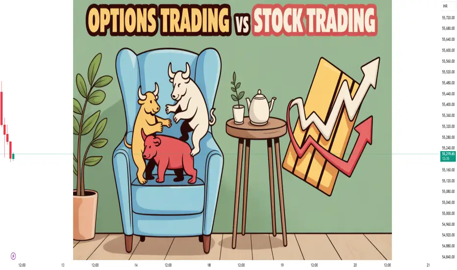
Options Trading vs Stock Trading1. Introduction
In financial markets, two of the most popular ways to trade are stock trading and options trading. While they may seem similar because they both involve securities listed on exchanges, they are fundamentally different in structure, risk, reward potential, and required skill level.
Think of stock trading as owning the house and options trading as renting or securing the right to buy/sell the house in the future. Both can make you money, but the way they work — and the risks they carry — are completely different.
In this guide, we’ll break down:
What each is and how it works
Key differences in ownership, leverage, and risk
Pros and cons of each
Which suits different types of traders and investors
Real-world examples and strategies
2. What is Stock Trading?
Definition
Stock trading is the buying and selling of shares in publicly listed companies. When you buy a stock, you own a piece of that company. This ownership comes with certain rights (like voting in shareholder meetings) and potential benefits (like dividends).
How It Works
You buy shares of a company on the stock exchange.
If the company grows and its value increases, the stock price goes up — you can sell for a profit.
If the company struggles, the stock price drops — you can incur losses.
You can hold stocks for minutes (day trading), months (swing trading), or years (investing).
Example:
If you buy 100 shares of Reliance Industries at ₹2,500 and the price rises to ₹2,700, your profit is:
ini
Copy
Edit
Profit = (2700 - 2500) × 100 = ₹20,000
3. What is Options Trading?
Definition
Options trading involves contracts that give you the right, but not the obligation, to buy or sell an asset (like a stock) at a specific price before a specific date.
Two Types of Options
Call Option – Right to buy at a set price (bullish view)
Put Option – Right to sell at a set price (bearish view)
Key Difference
Owning an option does not mean you own the stock — you own a derivative contract whose value is linked to the stock’s price.
Example:
You buy a call option for TCS with a strike price of ₹3,500 expiring in 1 month.
If TCS rises to ₹3,700, your option gains value — you can sell it for a profit without ever owning the stock.
4. Core Differences Between Stock and Options Trading
Feature Stock Trading Options Trading
Ownership You own part of the company You own a contract, not the company
Leverage Limited High leverage possible
Risk Can lose 100% if stock goes to zero Can lose entire premium (buyer) or face unlimited loss (seller)
Complexity Easier to understand More complex with multiple strategies
Capital Required Higher for large positions Lower due to leverage
Time Decay No time limit Value decreases as expiry nears
Profit Potential Unlimited upside (long), limited downside Can be structured for any market condition
Holding Period Can hold indefinitely Has fixed expiry dates
5. How You Make Money in Each
In Stock Trading
Price Appreciation – Buy low, sell high.
Dividends – Regular payouts from company profits.
Short Selling – Borrowing shares to sell at high prices and buying back lower.
In Options Trading
Buying Calls – Profit when stock price rises above strike + premium.
Buying Puts – Profit when stock price falls below strike - premium.
Writing (Selling) Options – Earn premium but take on obligation to buy/sell if exercised.
Spreads and Strategies – Combine options to profit in volatile, neutral, or directional markets.
6. Risk and Reward Profiles
Stock Trading Risk
Price risk: If the company fails, the stock can drop drastically.
Market risk: General downturns affect most stocks.
Overnight risk: News or global events can gap prices.
Reward:
Potential for significant gains if the company grows over time.
Options Trading Risk
For Buyers: Maximum loss is the premium paid; risk of total loss is high if market doesn’t move in time.
For Sellers: Potentially unlimited loss if market moves against you.
Time Decay: Options lose value as expiry approaches, hurting buyers but benefiting sellers.
Reward:
Leverage can lead to high percentage returns on small investments.
7. Leverage and Capital Efficiency
Stocks: To buy 100 shares of Infosys at ₹1,500, you need ₹1,50,000.
Options: You might control the same 100 shares with a call option costing ₹5,000–₹10,000.
Leverage means your returns can be multiplied, but so can your losses.
8. Liquidity and Flexibility
Stocks generally have high liquidity in large-cap companies.
Options can have lower liquidity, especially in far-out strikes or in less popular stocks.
Flexibility: Options allow hedging (protecting your stock position), creating income strategies, or betting on volatility.
9. Strategy Examples
Stock Trading Strategies
Buy and Hold
Swing Trading
Momentum Trading
Value Investing
Options Trading Strategies
Covered Call
Protective Put
Iron Condor
Straddle/Strangle
Bull Call Spread / Bear Put Spread
10. Taxes and Costs
In India, stock trades incur STT, brokerage, and capital gains tax.
Options trades incur STT on the premium, brokerage, and are taxed as business income for active traders.
11. Psychological Differences
Stock traders can afford to be more patient — long-term investing smooths out volatility.
Options traders face time pressure, making decision-making more intense.
Emotional discipline is more critical in options due to leverage and quick losses.
12. When to Choose Stocks vs Options
Scenario Better Choice
Long-term wealth building Stocks
Low capital but high return potential Options
Steady dividend income Stocks
Hedging a portfolio Options
Betting on short-term price moves Options
Lower stress, simpler approach Stocks
13. Common Mistakes
In Stock Trading
Chasing hot tips
Overtrading
Ignoring fundamentals
In Options Trading
Not understanding time decay
Overusing leverage
Selling naked calls without risk controls
14. Real-World Example Comparison
Let’s say HDFC Bank is trading at ₹1,500.
Stock Trade:
Buy 100 shares = ₹1,50,000 investment
If stock rises to ₹1,560, profit = ₹6,000 (4% return).
Options Trade:
Buy 1 call option (lot size 550 shares, premium ₹20) = ₹11,000 investment
If stock rises to ₹1,560, option premium might rise to ₹50:
Profit = ₹16,500 (150% return).
But if the stock doesn’t rise before expiry?
Stock trader loses nothing (unless price drops).
Option trader loses entire ₹11,000 premium.
15. The Bottom Line
Stock trading is ownership-based, simpler, and generally better for building long-term wealth.
Options trading is contract-based, more complex, and better suited for short-term speculation or hedging.
Both have roles in a smart trader’s toolkit — the key is knowing when and how to use each.
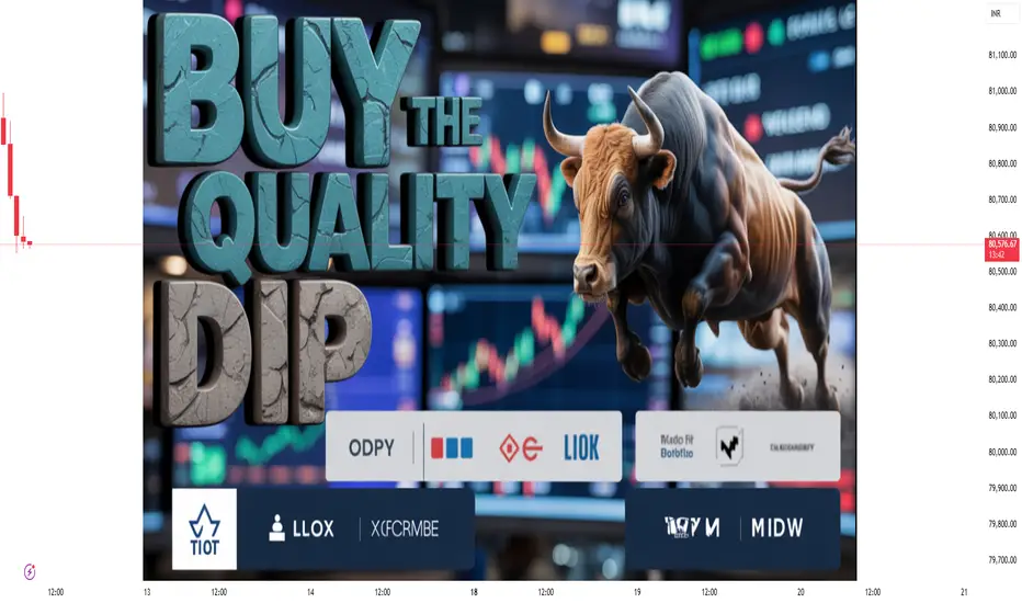
High-Quality Dip Buying1. Introduction – The Essence of Dip Buying
The phrase “Buy the dip” is one of the most common in financial markets — from Wall Street veterans to retail traders on social media. The core idea is simple:
When an asset’s price temporarily falls within an overall uptrend, smart traders buy at that lower price, expecting it to recover and make new highs.
But here’s the reality — not all dips are worth buying. Many traders rush in too soon, only to see the price fall further.
This is why High-Quality Dip Buying is different — it’s about buying dips with probability, timing, and market structure on your side, not just reacting to a red candle.
The goal here is strategic patience, technical confirmation, and risk-controlled execution.
2. Why Dip Buying Works (When Done Right)
Dip buying works because:
Trend Continuation – In a strong uptrend, pullbacks are natural pauses before the next leg higher.
Liquidity Pockets – Price often dips into zones where big players add positions.
Psychological Discounts – Market participants love “getting in at a better price,” creating buying pressure after a drop.
Mean Reversion – Markets often revert to an average after short-term overreactions.
But — without confirming the quality of the dip, traders risk catching a falling knife (a price that keeps dropping without support).
3. What Makes a “High-Quality” Dip?
A dip becomes high quality when:
It occurs in a strong underlying trend (measured with moving averages, higher highs/higher lows, or macro fundamentals).
The pullback is controlled, not panic-driven.
Volume behavior confirms accumulation — volume dries up during the dip and increases on recovery.
It tests a well-defined support zone (key levels, VWAP, 50-day MA, Fibonacci retracement, etc.).
Market sentiment remains bullish despite short-term weakness.
Macro or fundamental story stays intact — no major negative catalyst.
Think of it this way:
A low-quality dip is like buying a “discounted” product that’s broken.
A high-quality dip is like buying a brand-new iPhone during a holiday sale — same product, better price.
4. The Psychology Behind Dip Buying
Understanding trader psychology is critical.
Fear – When prices drop, many panic-sell. This creates opportunities for disciplined traders.
Greed – Some traders jump in too early without confirmation, leading to losses.
Patience – High-quality dip buyers wait for confirmation instead of guessing the bottom.
Confidence – They trust the trend and their plan, avoiding emotional exits.
In other words, dip buying rewards those who stay calm when others are reacting impulsively.
5. Market Conditions Where Dip Buying Thrives
High-quality dip buying works best in:
Strong Bull Markets – Indices and leading sectors are making higher highs.
Post-Correction Recoveries – Markets regain bullish momentum after a healthy pullback.
High-Liquidity Stocks/Assets – Blue chips, large caps, index ETFs, or top cryptos.
Clear Sector Leadership – Strong sectors (tech, healthcare, renewable energy) attract consistent dip buyers.
It’s risky in:
Bear markets (dips often turn into bigger drops)
Illiquid assets (wild volatility without strong support)
News-driven selloffs (fundamental damage)
6. Technical Tools for Identifying High-Quality Dips
A good dip buyer uses price action + indicators + volume.
a) Moving Averages
20 EMA / 50 EMA – Short to medium-term trend guides.
200 SMA – Long-term institutional trend.
High-quality dips often bounce near the 20 EMA in strong trends or the 50 EMA in moderate ones.
b) Support and Resistance Zones
Look for price retracing to:
Previous breakout levels
Trendline support
Volume profile high-volume nodes
c) Fibonacci Retracements
Common dip zones:
38.2% retracement – Healthy shallow pullback.
50% retracement – Neutral zone.
61.8% retracement – Deeper but often still bullish.
d) RSI (Relative Strength Index)
Strong trends often dip to RSI 40–50 before bouncing.
Avoid dips where RSI breaks below 30 and stays weak.
e) Volume Profile
Healthy dips = declining volume during pullback, rising volume on recovery.
7. Step-by-Step: Executing a High-Quality Dip Buy
Here’s a simple process:
Step 1 – Identify the Trend
Use moving averages and price structure (higher highs & higher lows).
Step 2 – Wait for the Pullback
Let price retrace to a strong support area.
Avoid chasing — patience is key.
Step 3 – Look for Confirmation
Reversal candlestick patterns (hammer, bullish engulfing).
Positive divergence in RSI/MACD.
Bounce on increased volume.
Step 4 – Plan Your Entry
Scale in: Start with partial size at the support, add on confirmation.
Use limit orders at planned levels.
Step 5 – Set Stop Loss
Place below recent swing low or key support.
Step 6 – Manage the Trade
Trail stop as price moves in your favor.
Take partial profits at predefined levels.
8. Risk Management in Dip Buying
Even high-quality dips can fail. Protect yourself by:
Never going all-in — scale in.
Using stop losses — don’t hold if structure breaks.
Sizing based on volatility — smaller size for volatile assets.
Limiting trades — avoid overtrading every dip.
9. Real Market Examples
Example 1 – Stock Market
Apple (AAPL) in a bull market often pulls back to the 20 EMA before continuing higher. Traders buying these dips with confirmation have historically seen strong returns.
Example 2 – Cryptocurrency
Bitcoin in a strong uptrend (2020–2021) had multiple 15–20% dips to the 50-day MA — each becoming an opportunity before making new highs.
Example 3 – Index ETFs
SPY ETF during 2019–2021 often dipped to the 50 EMA before strong rallies.
10. Common Mistakes in Dip Buying
Catching a falling knife — Buying without confirmation.
Ignoring news events — Buying into negative fundamental shifts.
Overleveraging — Increasing risk on a guess.
Buying every dip — Not all dips are equal.
No exit plan — Holding losers too long.
Conclusion
High-quality dip buying isn’t about impulsively buying when prices drop. It’s a disciplined, structured, and patient approach that aligns trend, technical analysis, and psychology.
When executed with precision and risk management, it allows traders to buy strength at a discount and participate in powerful trend continuations.
The golden rule?
Never buy a dip just because it’s lower — buy because the trend, structure, and confirmation all align.
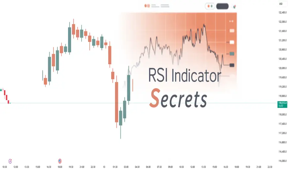
RSI Reversal Strategy 1. Introduction to RSI and Why Reversals Matter
In the world of trading, trends are exciting, but reversals are where many traders find their “gold mines.”
Why? Because reversals can catch market turning points before a new trend develops, giving you maximum profit potential from the very start of the move.
One of the most widely used tools to spot these turning points is the Relative Strength Index (RSI). Developed by J. Welles Wilder in 1978, the RSI measures the speed and magnitude of recent price changes to determine whether an asset is overbought or oversold.
In simple words:
RSI tells you when prices have gone too far, too fast, and may be ready to reverse.
It’s like a “market pressure gauge” — too much pressure on one side, and the price often snaps back.
The RSI Reversal Strategy uses these extreme readings to anticipate when a price trend is likely to stall and reverse direction.
2. The RSI Formula (for those who like the math)
While you don’t need to calculate RSI manually in modern charting platforms, it’s important to understand what’s going on under the hood:
𝑅
𝑆
𝐼
=
100
−
(
100
1
+
𝑅
𝑆
)
RSI=100−(
1+RS
100
)
Where:
RS = Average Gain over N periods ÷ Average Loss over N periods
N = The lookback period (commonly 14)
Interpretation:
RSI ranges from 0 to 100
Traditionally:
Above 70 = Overbought
Below 30 = Oversold
Extreme reversals are often spotted above 80 or below 20.
3. Why RSI Works for Reversals
Price movement isn’t random chaos — it’s driven by human behavior: fear, greed, panic, and FOMO.
When price rises too quickly, buyers eventually run out of fuel.
When price drops too sharply, sellers get exhausted.
The RSI measures momentum — and momentum always slows down before a reversal.
The RSI reversal logic is basically saying: “If this much buying or selling pressure was unsustainable before, it’s probably unsustainable now.”
4. Types of RSI Reversal Setups
There are several patterns you can use with RSI to detect reversals. Let’s go step-by-step.
4.1 Classic Overbought/Oversold Reversal
Idea:
When RSI > 70 (or 80), the asset may be overbought → look for short opportunities.
When RSI < 30 (or 20), the asset may be oversold → look for long opportunities.
Example Logic:
RSI crosses above 70 → wait for it to fall back below 70 → enter short.
RSI crosses below 30 → wait for it to climb back above 30 → enter long.
Pros: Very simple, beginner-friendly.
Cons: Works better in ranging markets, can fail in strong trends.
4.2 RSI Divergence Reversal
Idea:
Price makes a new high, but RSI fails to make a new high — or vice versa.
This signals that momentum is weakening, even though price hasn’t reversed yet.
Types:
Bearish Divergence: Price forms higher highs, RSI forms lower highs → possible top.
Bullish Divergence: Price forms lower lows, RSI forms higher lows → possible bottom.
Why it works: Divergence shows that momentum is not supporting the current price movement — a common pre-reversal sign.
4.3 RSI Failure Swing
Idea:
An RSI reversal where the indicator attempts to re-test an extreme level but fails.
Bullish Failure Swing:
RSI drops below 30 (oversold)
RSI rises above 30, then drops again but stays above 30
RSI then breaks the previous high → bullish signal
Bearish Failure Swing:
RSI rises above 70 (overbought)
RSI drops below 70, then rises again but stays below 70
RSI then breaks the previous low → bearish signal
4.4 RSI Reversal Zone Strategy
Idea:
Instead of only looking at 30/70, use custom zones like 20/80 or 25/75 to filter out false signals in trending markets.
5. Timeframes and Market Suitability
RSI works in all markets — stocks, forex, crypto, commodities — but the effectiveness changes with the timeframe.
Scalping/Intraday: 1-min, 5-min, 15-min → RSI 7 or RSI 14 with tighter zones (20/80)
Swing Trading: 1H, 4H, Daily → RSI 14 standard settings
Position Trading: Daily, Weekly → RSI 14 or 21 for smoother signals
Tip:
Shorter timeframes = more signals, but more noise.
Longer timeframes = fewer signals, but stronger reliability.
6. Complete RSI Reversal Strategy Rules (Basic Version)
Let’s build a straightforward rule set.
Parameters:
RSI period: 14
Zones: 30 (oversold), 70 (overbought)
Buy Setup:
RSI drops below 30
RSI rises back above 30
Confirm with price action (e.g., bullish engulfing candle)
Stop-loss below recent swing low
Take profit at 1:2 risk-reward or when RSI nears 70
Sell Setup:
RSI rises above 70
RSI drops back below 70
Confirm with price action (e.g., bearish engulfing candle)
Stop-loss above recent swing high
Take profit at 1:2 risk-reward or when RSI nears 30
7. Advanced RSI Reversal Strategy Enhancements
A pure RSI reversal system can be prone to false signals, especially during strong trends. Here’s how to improve it:
7.1 Combine with Support & Resistance
Only take RSI oversold longs near a support zone.
Only take RSI overbought shorts near a resistance zone.
7.2 Add Volume Confirmation
Look for volume spikes or unusual activity when RSI hits reversal zones — stronger reversal probability.
7.3 Use Multiple Timeframe Confirmation
If you see an RSI reversal on a 15-min chart, check the 1H chart.
When both timeframes align, the reversal is more likely to work.
7.4 Combine with Candlestick Patterns
Reversal candlestick patterns like:
Hammer / Inverted Hammer
Doji
Engulfing
Morning/Evening Star
… can make RSI signals much more reliable.
7.5 RSI Trendline Breaks
Draw trendlines directly on RSI. If RSI breaks its own trendline, it can signal an early reversal before price follows.
8. Risk Management for RSI Reversal Trading
Even the best reversal setups fail sometimes — especially in strong trends where RSI can stay overbought or oversold for a long time.
Golden Rules:
Never risk more than 1–2% of your capital on a single trade.
Always place a stop-loss — don’t assume the reversal will happen immediately.
Use a risk-reward ratio of at least 1:2.
Avoid revenge trading after a loss — overtrading is the #1 account killer.
9. Example Trade Walkthrough
Let’s go through a bullish RSI reversal trade on a stock.
Market: Reliance Industries (Daily chart)
Observation: RSI drops to 22 (extremely oversold) while price nears a major support level from last year.
Trigger: RSI crosses back above 30 with a bullish engulfing candle on the daily chart.
Entry: ₹2,350
Stop-loss: ₹2,280 (below swing low)
Target: ₹2,500 (risk-reward ~1:2)
Result: Price rallies to ₹2,520 in 7 trading days.
10. Common Mistakes to Avoid
Using RSI blindly without price action
RSI needs context — never enter just because it’s overbought or oversold.
Trading against strong trends
RSI can stay extreme for a long time; wait for price action confirmation.
Too small timeframes for beginners
Lower timeframes have too much noise — start with daily/4H charts.
Ignoring market news
Fundamental events can invalidate technical signals instantly.
Conclusion
The RSI Reversal Strategy is powerful because it taps into one of the most consistent behaviors in the market — momentum exhaustion.
When applied with proper filters like support/resistance, candlestick confirmation, and disciplined risk management, it can become a high-probability trading edge.
However — and this is key — no strategy is bulletproof. The RSI Reversal Strategy will fail sometimes, especially in parabolic moves or during strong news-driven trends. Your long-term success depends on how well you manage risk and filter bad signals.
Think of RSI as your early warning radar, not an autopilot. Let it tell you when to pay attention, then confirm with your trading plan before taking action.
Part7 Trading Master ClassPractical Tips for Success
Backtest strategies on historical data.
Start with paper trading before using real money.
Track your trades in a journal.
Combine technical analysis with options knowledge.
Trade liquid options with tight bid-ask spreads.
Final Thoughts
Options are like a Swiss Army knife in trading — versatile, powerful, and potentially dangerous if misused. The right strategy depends on:
Market view (up, down, sideways, volatile, stable)
Risk tolerance
Timeframe
Experience level
By starting with basic strategies like covered calls or protective puts, then moving into spreads, straddles, and condors, you can build a strong foundation. With practice, risk management, and discipline, options trading can be a valuable tool in your investment journey.

Part12 Trading Master ClassAdvanced Options Strategies
Butterfly Spread
When to Use: Expect stock to stay near a specific price.
How It Works: Buy 1 ITM option, sell 2 ATM options, buy 1 OTM option.
Risk: Limited.
Reward: Highest if stock ends at middle strike.
Example: Stock ₹100, buy call ₹95, sell 2 calls ₹100, buy call ₹105.
Calendar Spread
When to Use: Expect low short-term volatility but possible long-term move.
How It Works: Sell short-term option, buy long-term option at same strike.
Risk: Limited to net premium.
Reward: Comes from time decay of short option.

Part4 Institutional TradingStraddle
When to Use: Expect big move but unsure direction.
How It Works: Buy call and put at same strike & expiry.
Risk: High premium cost.
Reward: Big if price moves sharply up or down.
Example: Stock at ₹100, buy call ₹100 (₹4) and put ₹100 (₹4). Cost ₹8. Needs a big move to profit.
Strangle
When to Use: Expect big move but want cheaper entry than straddle.
How It Works: Buy OTM call and put.
Risk: Cheaper than straddle but needs larger move.
Example: Stock at ₹100, buy call ₹105 (₹3) and put ₹95 (₹3). Cost ₹6.
Iron Condor
When to Use: Expect low volatility.
How It Works: Sell an OTM call spread + sell an OTM put spread.
Risk: Limited by spread width.
Reward: Limited to premium collected.
Example: Stock at ₹100, sell call ₹110, buy call ₹115; sell put ₹90, buy put ₹85.

Part2 Ride The Big Moves Intermediate Options Strategies
Bull Call Spread
When to Use: Expect moderate price rise.
How It Works: Buy a call at a lower strike, sell a call at higher strike.
Risk: Limited to net premium paid.
Reward: Limited to strike difference minus premium.
Example: Buy call at ₹100 (₹5), sell call at ₹110 (₹2). Net cost ₹3. Max profit ₹7.
Bear Put Spread
When to Use: Expect moderate decline.
How It Works: Buy put at higher strike, sell put at lower strike.
Risk: Limited to net premium paid.
Reward: Limited but cheaper than buying a single put.
Example: Buy put ₹105 (₹6), sell put ₹95 (₹3). Net cost ₹3. Max profit ₹7.

Part9 Trading Master Class Why Traders Use Options
Options aren’t just for speculation — they have multiple uses:
Speculation – Betting on price moves.
Hedging – Protecting an existing investment from loss.
Income Generation – Selling options for premium income.
Risk Management – Limiting losses through defined-risk trades.
Basic Options Strategies (Beginner Level)
Buying Calls
When to Use: You expect the price to go up.
How It Works: You buy a call option to lock in a lower purchase price.
Risk: Limited to the premium paid.
Reward: Unlimited upside.
Example: Stock at ₹100, buy a call at ₹105 strike for ₹3 premium. If stock rises to ₹120, your profit = ₹12 – ₹3 = ₹9 per share.

Psychology & Risk Management in Trading 1. Introduction
Trading is often thought of as a purely numbers-driven game — charts, technical indicators, fundamental analysis, and economic data. But in reality, the true battlefield is inside your head. Two traders can have access to the exact same market data, yet end up with completely different results. The difference lies in psychology and risk management.
Psychology determines how you make decisions under pressure.
Risk management determines whether you survive long enough to benefit from good decisions.
Think of trading as a three-legged stool:
Strategy – Your technical/fundamental system for entering and exiting trades.
Psychology – Your ability to stick to the plan under real conditions.
Risk Management – Your safeguard against catastrophic loss.
If one leg is missing, the stool collapses. A profitable strategy without psychological discipline becomes useless. A strong mindset without proper risk controls eventually faces ruin. And perfect risk management without skill or discipline simply results in slow losses.
Our goal here is to align mindset with money management for long-term success.
2. Understanding Trading Psychology
2.1. Why Psychology Matters More Than You Think
When you’re trading, money is not just numbers — it represents:
Security (fear of losing it)
Freedom (desire to win more)
Ego (feeling smart or dumb based on market outcomes)
This emotional attachment creates mental biases that cloud judgment. Unlike a chessboard, the market is an uncertain game — the same move can lead to a win or loss depending on external forces beyond your control.
The primary enemy is not “the market,” but you:
Closing winning trades too early out of fear.
Holding onto losing trades hoping they’ll recover.
Overtrading to “make back” losses.
Avoiding valid setups after a losing streak.
2.2. The Main Psychological Biases in Trading
1. Loss Aversion
Humans hate losing more than they like winning. Research shows losing $100 feels twice as bad as gaining $100 feels good.
In trading, this causes:
Refusing to take stop losses.
Adding to losing positions to “average down.”
2. Overconfidence Bias
After a streak of wins, traders often overestimate their skill.
Example: Turning a $1,000 account into $2,000 in a week might lead to doubling trade size without a valid reason.
3. Confirmation Bias
Seeking only information that supports your existing view. If you’re bullish on gold, you might only read bullish news and ignore bearish signals.
4. Recency Bias
Giving too much weight to recent events. A trader who just experienced a big rally might expect it to continue, ignoring long-term resistance levels.
5. Fear of Missing Out (FOMO)
Jumping into trades without proper analysis because you see the market moving.
6. Revenge Trading
Trying to “get back” at the market after a loss by taking impulsive trades.
2.3. Emotional States and Their Effects
Fear – Leads to hesitation, missed opportunities, and premature exits.
Greed – Leads to over-leveraging and chasing setups.
Hope – Keeps traders in losing trades far longer than necessary.
Regret – Causes paralysis, stopping you from entering new opportunities.
Euphoria – False sense of invincibility, leading to reckless trades.
3. Mastering the Trader’s Mindset
3.1. Accepting Uncertainty
Markets are probabilistic, not certain. The best trade setups still lose sometimes. The key is to think in terms of probabilities, not certainties.
Mental shift:
Bad trade ≠ losing trade.
Good trade ≠ winning trade.
A “good trade” is one where you followed your plan and managed risk — regardless of the outcome.
3.2. Developing Discipline
Discipline means doing what your trading plan says every time, even when you feel like doing otherwise.
Practical ways to build discipline:
Pre-market checklist (entry/exit rules, risk per trade, market conditions).
Post-trade review to identify emotional decisions.
Simulated trading to practice following rules without monetary pressure.
3.3. Managing Emotional Cycles
Traders often go through repeated emotional phases:
Excitement – New strategy, first wins.
Euphoria – Overconfidence and overtrading.
Fear/Panic – Sharp drawdown after reckless trades.
Desperation – Trying to recover losses quickly.
Resignation – Stepping back, reevaluating.
Rebuilding – Adopting better discipline.
Your goal is to flatten the cycle, reducing extreme highs and lows.
4. Risk Management: The Survival Mechanism
4.1. The Goal of Risk Management
Trading is not about avoiding losses — losses are inevitable. The aim is to control the size of your losses so they don’t destroy your capital or confidence.
4.2. The Three Pillars of Risk Management
1. Position Sizing
Determine how much capital to risk per trade. Common rules:
Risk only 1–2% of total capital on any single trade.
Example: If you have ₹1,00,000 and risk 1% per trade, your max loss is ₹1,000.
2. Stop Losses
Predetermined exit points to limit losses.
Hard stops – Fixed at a price level.
Trailing stops – Move with the trade to lock in profits.
3. Risk-Reward Ratio
A measure of potential reward vs. risk.
Example:
Risk: ₹500
Potential Reward: ₹1,500
R:R = 1:3 (good)
4.3. The Power of Capital Preservation
Here’s why big losses are dangerous:
Lose 10% → Need 11% gain to recover.
Lose 50% → Need 100% gain to recover.
The bigger the loss, the harder the comeback. Capital preservation should be your #1 priority.
4.4. Avoiding Overleveraging
Leverage magnifies both gains and losses. Many traders blow accounts not because their strategy was bad, but because they used excessive leverage.
5. Integrating Psychology with Risk Management
5.1. The Feedback Loop
Poor psychology → Poor risk decisions → Bigger losses → Worse psychology.
You must break the loop by locking in good risk rules before trading.
5.2. The Risk Management Mindset
Treat each trade as just one of thousands you’ll make.
Focus on execution quality, not daily P/L.
Celebrate following your plan, not just winning.
5.3. Journaling
A trading journal should include:
Entry/exit points and reasons.
Risk per trade.
Emotional state before/during/after.
Lessons learned.
Over time, patterns emerge that reveal weaknesses in both mindset and risk control.
6. Practical Tips for Building Psychological Strength
Meditation & Mindfulness – Keeps emotions in check.
Physical Health – A healthy body supports a calm mind.
Sleep – Fatigue increases impulsive decisions.
Routine – Structured trading hours reduce stress.
Detach from P/L – Judge performance over months, not days.
7. Case Studies: When Psychology Meets Risk
Case Study 1 – The Overconfident Scalper
Wins 10 trades in a row, doubles position size.
One loss wipes out previous gains.
Lesson: Stick to fixed risk % per trade regardless of winning streaks.
Case Study 2 – The Hopeful Investor
Holds losing position for months.
Avoids taking stop loss because “it’ll recover.”
Lesson: Hope is not a strategy; use predefined exits.
8. Conclusion
Trading success is 20% strategy and 80% mindset + risk control. The market will always test your patience, discipline, and emotional control. By mastering your psychology and implementing rock-solid risk management, you give yourself the best chance not just to make money — but to stay in the game long enough to grow it.

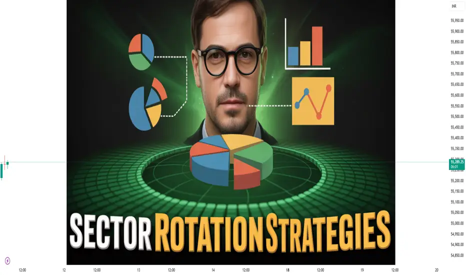
Sector Rotation Strategies1. Introduction: What is Sector Rotation?
Imagine the stock market as a giant relay race, but instead of runners passing a baton, it’s different sectors of the economy passing investment leadership to each other. Sometimes technology stocks sprint ahead, other times energy stocks lead the race, then maybe healthcare takes the spotlight. This cyclical shift in market leadership is what traders call Sector Rotation.
Sector rotation strategies aim to predict and act on these shifts, moving money into sectors expected to outperform and out of sectors likely to underperform.
It’s based on one powerful observation:
Not all sectors move in the same direction at the same time.
Even during bull markets, some sectors outperform others. And during bear markets, some sectors lose less (or even gain).
By aligning investments with economic cycles, market sentiment, and sector strength, traders and investors can potentially generate higher returns with lower risk.
2. Why Sector Rotation Works
The strategy works because different sectors benefit from different phases of the economic and market cycle:
Economic Growth boosts certain sectors (e.g., consumer discretionary, technology).
Recession or slowdown benefits defensive sectors (e.g., utilities, healthcare).
Inflationary spikes benefit commodities and energy.
Falling interest rates favor growth-oriented sectors.
The key driver here is capital flow. Big institutional investors (mutual funds, pension funds, hedge funds) don’t move all at once into the whole market — they rotate capital into sectors they expect to lead based on macroeconomic forecasts, earnings trends, and market psychology.
3. The Core Concept: The Economic Cycle & Sector Leadership
Sector rotation is deeply tied to business cycles. A typical economic cycle has four main stages:
Early Expansion (Recovery phase)
Mid Expansion (Growth phase)
Late Expansion (Overheating phase)
Recession (Contraction phase)
Here’s how different sectors tend to perform in each phase:
Phase Economic Traits Leading Sectors
Early Expansion Low interest rates, GDP growth starting, optimism Technology, Consumer Discretionary, Industrials
Mid Expansion Strong growth, rising demand, stable inflation Materials, Energy, Financials
Late Expansion Inflation rising, interest rates climbing Energy, Materials, Commodities
Recession Slowing growth, high unemployment, fear Healthcare, Utilities, Consumer Staples
This isn’t a fixed law — think of it as probabilities, not certainties.
4. Offensive vs Defensive Sectors
Sectors can broadly be divided into offensive (cyclical) and defensive (non-cyclical) categories.
Offensive (Cyclical) Sectors
Technology
Consumer Discretionary
Industrials
Financials
Materials
Energy
These sectors perform best when the economy is growing and consumers/businesses are spending.
Defensive (Non-Cyclical) Sectors
Healthcare
Utilities
Consumer Staples
Telecommunications
These sectors provide steady demand regardless of economic conditions.
5. Tools & Indicators for Sector Rotation
To implement a sector rotation strategy, traders use data-driven analysis combined with macroeconomic observation. Here are the main tools:
5.1 Relative Strength Analysis (RS)
Compare sector ETFs or indexes against a benchmark (e.g., S&P 500).
Tools: Relative Strength Ratio (RSI of sector performance vs market).
5.2 Economic Indicators
GDP Growth Rate
Interest Rates (Fed rate hikes/cuts)
Inflation trends
Consumer Confidence Index
PMI (Purchasing Managers Index)
5.3 Market Breadth & Momentum
Advance/Decline Line
Moving Averages (50, 200-day)
MACD for sector ETFs
5.4 ETF & Index Tracking
Commonly used sector ETFs in the U.S.:
XLK – Technology
XLY – Consumer Discretionary
XLF – Financials
XLE – Energy
XLV – Healthcare
XLP – Consumer Staples
XLU – Utilities
6. Sector Rotation Strategies in Practice
6.1 Top-Down Approach
Analyze macroeconomic conditions (Are we in early expansion? Late cycle?).
Identify sectors likely to lead in that stage.
Select strong stocks within those leading sectors.
Example:
If GDP is growing and interest rates are low, technology and consumer discretionary sectors might lead. Pick top-performing stocks in those sectors.
6.2 Momentum-Based Rotation
Rotate into sectors showing the strongest short- to medium-term performance.
Exit sectors showing weakening momentum.
6.3 Seasonality Rotation
Some sectors perform better at certain times of the year (e.g., retail in Q4 due to holiday shopping).
6.4 Quantitative Rotation
Use algorithms and backtesting to determine optimal rotation intervals and triggers.
7. The Intermarket Connection
Sector rotation doesn’t exist in isolation — it’s linked to bonds, commodities, and currencies.
Bond yields rising → Favors financials (banks earn more on lending spreads).
Oil prices rising → Benefits energy sector, hurts transportation.
Strong dollar → Hurts export-heavy sectors, benefits importers.
8. Real-World Examples of Sector Rotation
Example 1: Post-COVID Recovery (2020–2021)
Early 2020: Pandemic crash → Defensive sectors like healthcare, utilities outperformed.
Mid 2020–2021: Recovery & stimulus → Tech, consumer discretionary, and financials surged.
Late 2021: Inflation & rate hikes talk → Energy and materials took the lead.
Example 2: High Inflation Period (2022)
Fed rate hikes → Tech underperformed.
Energy and utilities outperformed.
Defensive sectors cushioned losses during market drops.
9. Risks & Limitations of Sector Rotation
Timing Risk: Entering a sector too early or too late can lead to losses.
False Signals: Economic data is often revised; market sentiment can override fundamentals.
Transaction Costs & Taxes: Frequent rotation = higher costs.
Over-Optimization: Backtested strategies may fail in real-world conditions.
10. Building Your Own Sector Rotation Strategy
Here’s a simple framework:
Determine the Market Cycle:
Look at GDP trends, inflation, interest rates, unemployment.
Select Likely Winning Sectors:
Use RS analysis and sector ETF charts.
Confirm with Technicals:
Moving averages, momentum oscillators.
Choose Best-in-Class Stocks or ETFs:
Pick leaders with strong fundamentals and technical setups.
Set Exit Rules:
RS weakening? Macro shift? Hit stop-loss.
Conclusion
Sector Rotation Strategies are not about predicting the market perfectly — they’re about stacking probabilities in your favor by aligning with the strongest sectors in the prevailing economic climate.
When done right:
You ride the wave of sector leadership instead of fighting it.
You reduce risk by avoiding weak sectors.
You improve performance by capturing the strongest trends.
Remember:
The stock market isn’t one giant boat — it’s a fleet of ships. Some sail faster in certain winds, some slow down. Sector rotation is simply choosing the right ship at the right time.
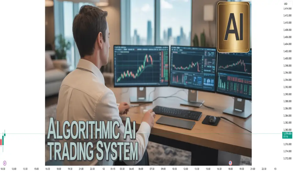
AI-Powered Algorithmic Trading 1. Introduction: The Fusion of AI and Algorithmic Trading
Algorithmic trading (or algo trading) refers to the use of computer programs to execute trading orders based on pre-defined rules. These rules can be based on timing, price, quantity, or any mathematical model.
Traditionally, algorithms were static—they executed strategies exactly as they were coded, without adapting to market changes in real time.
AI-powered algorithmic trading is different.
It integrates machine learning (ML) and artificial intelligence (AI) into trading systems, making them dynamic, adaptive, and self-improving.
Instead of blindly following a fixed script, an AI algorithm can:
Learn from historical market data
Identify evolving patterns
Adjust strategies based on changing conditions
Predict potential price movements
Manage risk dynamically
The result?
Trading systems that behave more like experienced human traders—except they operate at lightning speed and can process massive datasets in real time.
2. Why AI is Revolutionizing Algorithmic Trading
Before AI, algorithmic trading was powerful but rigid. If market conditions changed drastically—say, during a financial crisis or a geopolitical shock—the system might fail, simply because it was designed for "normal" conditions.
AI changes that by:
Pattern recognition: Detecting non-obvious market correlations.
Natural language processing (NLP): Interpreting news, earnings reports, and even social media sentiment in real-time.
Reinforcement learning: Learning from past trades and improving performance over time.
Adaptability: Shifting strategies instantly when volatility spikes or liquidity dries up.
In essence, AI empowers trading algorithms to think, not just follow orders.
3. Core Components of AI-Powered Algorithmic Trading Systems
To understand how these systems work, let’s break down the core building blocks:
3.1 Data Collection and Preprocessing
AI thrives on data—without quality data, even the most advanced AI model will fail.
Sources include:
Historical price data (open, high, low, close, volume)
Order book data (bid/ask depth)
News headlines & articles
Social media (Twitter, Reddit, StockTwits sentiment)
Macroeconomic indicators (interest rates, GDP growth, inflation)
Alternative data (satellite images, credit card transactions, shipping data)
Data preprocessing involves:
Cleaning: Removing errors or irrelevant information
Normalization: Scaling data for AI models
Feature engineering: Creating meaningful variables from raw data (e.g., moving averages, RSI, volatility)
3.2 Machine Learning Models
The heart of AI trading lies in ML models. Some popular ones include:
Supervised learning: Models like linear regression, random forests, or neural networks that predict future prices based on labeled historical data.
Unsupervised learning: Clustering methods to find patterns in unlabeled data (e.g., grouping similar trading days).
Reinforcement learning (RL): The AI learns optimal strategies through trial and error, receiving rewards for profitable trades.
Deep learning: Advanced neural networks (CNNs, LSTMs, Transformers) to handle complex time-series data and sentiment analysis.
3.3 Trading Strategy Generation
AI models help generate or refine strategies such as:
Trend-following (moving average crossovers)
Mean reversion (buying dips, selling rallies)
Statistical arbitrage (pairs trading, cointegration strategies)
Market making (providing liquidity and profiting from the bid-ask spread)
Event-driven (earnings surprises, mergers, economic announcements)
AI adds a twist—it can:
Adjust parameters dynamically
Identify optimal holding periods
Combine multiple strategies for diversification
3.4 Execution Algorithms
Once a trading signal is generated, execution algorithms ensure it’s carried out efficiently:
VWAP (Volume-Weighted Average Price) – Executes to match market volume patterns
TWAP (Time-Weighted Average Price) – Executes evenly over time
Implementation Shortfall – Balances execution cost vs. risk
Sniper/Stealth Orders – Hide large orders to avoid moving the market
AI improves execution by:
Predicting short-term order book dynamics
Avoiding periods of low liquidity
Detecting spoofing or manipulation
3.5 Risk Management
Risk is the biggest enemy in trading. AI systems incorporate:
Dynamic position sizing – Adjusting trade size based on volatility
Stop-loss adaptation – Moving stops based on changing conditions
Portfolio optimization – Balancing risk across multiple assets
Stress testing – Simulating extreme scenarios
AI models can predict drawdowns before they happen and adjust exposure accordingly.
4. Advantages of AI-Powered Algorithmic Trading
Speed: Executes trades in milliseconds.
Scalability: Can trade hundreds of assets simultaneously.
Objectivity: Removes human emotions like fear and greed.
Complex analysis: Processes terabytes of data that humans cannot.
Adaptability: Learns and evolves in real-time.
5. Challenges and Risks
AI isn’t a magic bullet—it comes with challenges:
Overfitting: AI may perform well on historical data but fail in real markets.
Black box problem: Deep learning models can be hard to interpret.
Data quality risk: Garbage in = garbage out.
Market regime shifts: AI models may fail in unprecedented situations.
Regulatory concerns: AI-driven trading must comply with strict financial regulations.
6. AI in Action – Real-World Use Cases
6.1 Hedge Funds
Firms like Renaissance Technologies and Two Sigma leverage AI for predictive modeling, order execution, and portfolio optimization.
6.2 High-Frequency Trading (HFT)
Firms deploy AI to detect microsecond price inefficiencies and exploit them before competitors.
6.3 Retail Trading Platforms
AI bots now help retail traders (e.g., Trade Ideas, TrendSpider) identify high-probability setups.
6.4 Sentiment-Driven Trading
AI scans Twitter, news feeds, and even Reddit forums to detect shifts in sentiment and trade accordingly.
7. Future Trends in AI-Powered Algorithmic Trading
Explainable AI (XAI): Making AI decisions transparent for regulators and traders.
Quantum computing integration: For lightning-fast optimization.
AI + Blockchain: Decentralized trading strategies and data verification.
Autonomous trading ecosystems: Fully self-managing portfolios with zero human intervention.
Cross-market intelligence: AI detecting correlations between equities, forex, commodities, and crypto in real-time.
8. Building Your Own AI-Powered Trading System – Step-by-Step
For traders who want to experiment:
Data sourcing: Choose reliable APIs (e.g., Alpha Vantage, Polygon.io, Quandl).
Choose a framework: Python (TensorFlow, PyTorch, scikit-learn) or R.
Feature engineering: Create technical and sentiment-based indicators.
Model training: Use supervised learning for prediction or reinforcement learning for strategy optimization.
Backtesting: Test strategies on historical data with realistic transaction costs.
Paper trading: Simulate live markets without risking real money.
Live deployment: Start with small capital and scale gradually.
Continuous learning: Update models with new data frequently.
9. Ethical & Regulatory Considerations
AI can cause market disruptions if misused:
Flash crashes: Rapid, AI-triggered selling can collapse prices.
Market manipulation: AI could unintentionally engage in manipulative patterns.
Bias in models: If training data is biased, trading decisions could be skewed.
Regulatory oversight: Authorities like SEBI (India), SEC (USA), and ESMA (Europe) monitor algorithmic trading closely.
10. Final Thoughts
AI-powered algorithmic trading is not just a technological leap—it’s a paradigm shift in how markets operate.
The combination of speed, intelligence, and adaptability makes AI an indispensable tool for modern traders and institutions.
However, successful deployment requires:
Robust data pipelines
Sound risk management
Ongoing monitoring and adaptation
In the right hands, AI can be a consistent alpha generator. In the wrong hands, it can be a high-speed path to losses.
The future will likely see more human-AI collaboration, where AI handles data-driven decisions and humans provide oversight, creativity, and strategic vision.
Options Trading Strategies 1. Introduction to Options Trading
Options are like a financial “contract” that gives you rights but not obligations.
When you buy an option, you are buying the right to buy or sell an asset at a specific price before a certain date.
They’re mainly used in stocks, commodities, indexes, and currencies.
Two main types of options:
Call Option – Right to buy an asset at a set price.
Put Option – Right to sell an asset at a set price.
Key terms:
Strike Price – The price at which you can buy/sell the asset.
Expiration Date – The last day you can use the option.
Premium – Price paid to buy the option.
In the Money (ITM) – Option has intrinsic value.
Out of the Money (OTM) – Option has no intrinsic value yet.
At the Money (ATM) – Strike price equals current market price.
Options give traders flexibility, leverage, and hedging power. But with great power comes great “margin calls” if you misuse them.
2. Why Traders Use Options
Options aren’t just for speculation — they have multiple uses:
Speculation – Betting on price moves.
Hedging – Protecting an existing investment from loss.
Income Generation – Selling options for premium income.
Risk Management – Limiting losses through defined-risk trades.
3. Basic Options Strategies (Beginner Level)
3.1 Buying Calls
When to Use: You expect the price to go up.
How It Works: You buy a call option to lock in a lower purchase price.
Risk: Limited to the premium paid.
Reward: Unlimited upside.
Example: Stock at ₹100, buy a call at ₹105 strike for ₹3 premium. If stock rises to ₹120, your profit = ₹12 – ₹3 = ₹9 per share.
3.2 Buying Puts
When to Use: You expect the price to go down.
How It Works: You buy a put option to sell at a higher price later.
Risk: Limited to the premium.
Reward: Significant (but capped at the strike price minus premium).
Example: Stock at ₹100, buy a put at ₹95 for ₹2 premium. If stock drops to ₹80, profit = ₹15 – ₹2 = ₹13.
3.3 Covered Call
When to Use: You own the stock but expect it to stay flat or slightly rise.
How It Works: Sell a call option against your owned stock to collect premium.
Risk: You must sell the stock if price exceeds strike.
Reward: Stock appreciation + premium income.
Example: Own stock at ₹100, sell call at ₹105 for ₹2. If stock stays below ₹105, you keep the ₹2.
3.4 Protective Put
When to Use: You own a stock and want downside protection.
How It Works: Buy a put to protect against price drops.
Risk: Premium cost.
Reward: Security against big losses.
Example: Own stock at ₹100, buy put at ₹95 for ₹2. Even if stock crashes to ₹50, you can still sell at ₹95.
4. Intermediate Options Strategies
4.1 Bull Call Spread
When to Use: Expect moderate price rise.
How It Works: Buy a call at a lower strike, sell a call at higher strike.
Risk: Limited to net premium paid.
Reward: Limited to strike difference minus premium.
Example: Buy call at ₹100 (₹5), sell call at ₹110 (₹2). Net cost ₹3. Max profit ₹7.
4.2 Bear Put Spread
When to Use: Expect moderate decline.
How It Works: Buy put at higher strike, sell put at lower strike.
Risk: Limited to net premium paid.
Reward: Limited but cheaper than buying a single put.
Example: Buy put ₹105 (₹6), sell put ₹95 (₹3). Net cost ₹3. Max profit ₹7.
4.3 Straddle
When to Use: Expect big move but unsure direction.
How It Works: Buy call and put at same strike & expiry.
Risk: High premium cost.
Reward: Big if price moves sharply up or down.
Example: Stock at ₹100, buy call ₹100 (₹4) and put ₹100 (₹4). Cost ₹8. Needs a big move to profit.
4.4 Strangle
When to Use: Expect big move but want cheaper entry than straddle.
How It Works: Buy OTM call and put.
Risk: Cheaper than straddle but needs larger move.
Example: Stock at ₹100, buy call ₹105 (₹3) and put ₹95 (₹3). Cost ₹6.
4.5 Iron Condor
When to Use: Expect low volatility.
How It Works: Sell an OTM call spread + sell an OTM put spread.
Risk: Limited by spread width.
Reward: Limited to premium collected.
Example: Stock at ₹100, sell call ₹110, buy call ₹115; sell put ₹90, buy put ₹85.
5. Advanced Options Strategies
5.1 Butterfly Spread
When to Use: Expect stock to stay near a specific price.
How It Works: Buy 1 ITM option, sell 2 ATM options, buy 1 OTM option.
Risk: Limited.
Reward: Highest if stock ends at middle strike.
Example: Stock ₹100, buy call ₹95, sell 2 calls ₹100, buy call ₹105.
5.2 Calendar Spread
When to Use: Expect low short-term volatility but possible long-term move.
How It Works: Sell short-term option, buy long-term option at same strike.
Risk: Limited to net premium.
Reward: Comes from time decay of short option.
5.3 Ratio Spread
When to Use: Expect limited move in one direction.
How It Works: Buy 1 option, sell multiple options at different strikes.
Risk: Unlimited on one side if not hedged.
5.4 Diagonal Spread
When to Use: Expect gradual move over time.
How It Works: Buy long-term option at one strike, sell short-term option at different strike.
6. Risk Management in Options
Even though options can limit loss, traders often misuse them and blow accounts.
Key risk tips:
Never risk more than 2–3% of capital on one trade.
Understand implied volatility — high IV inflates premiums.
Avoid selling naked options without sufficient margin.
Always set stop-loss rules.
7. Understanding Greeks (The DNA of Options Pricing)
Delta – How much the option price changes per ₹1 move in stock.
Gamma – How fast delta changes.
Theta – Time decay rate.
Vega – Sensitivity to volatility changes.
Rho – Interest rate sensitivity.
Mastering the Greeks means you understand why your option is moving, not just that it’s moving.
8. Common Mistakes to Avoid
Holding OTM options too close to expiry hoping for a miracle.
Selling naked calls without understanding unlimited risk.
Over-leveraging with too many contracts.
Ignoring commissions and slippage.
Not adjusting positions when market changes.
9. Practical Tips for Success
Backtest strategies on historical data.
Start with paper trading before using real money.
Track your trades in a journal.
Combine technical analysis with options knowledge.
Trade liquid options with tight bid-ask spreads.
10. Final Thoughts
Options are like a Swiss Army knife in trading — versatile, powerful, and potentially dangerous if misused. The right strategy depends on:
Market view (up, down, sideways, volatile, stable)
Risk tolerance
Timeframe
Experience level
By starting with basic strategies like covered calls or protective puts, then moving into spreads, straddles, and condors, you can build a strong foundation. With practice, risk management, and discipline, options trading can be a valuable tool in your investment journey.
Part4 Institutional TradingRisk Management in Strategies
Never sell naked calls unless fully hedged.
Position size to avoid overexposure.
Use stop-loss or delta hedging.
Monitor implied volatility — don’t sell cheap, don’t buy expensive.
12. Strategy Selection Framework
Market View: Bullish, Bearish, Neutral, Volatile?
Volatility Level: High IV (sell premium), Low IV (buy premium).
Capital & Risk Tolerance: Large capital allows complex spreads.
Time Frame: Short-term events vs. long-term trends.
Common Mistakes to Avoid
Trading without an exit plan.
Ignoring liquidity (wide bid-ask spreads hurt).
Selling options without understanding margin.
Overtrading during high emotions.
Not adjusting when market changes.
Advanced Adjustments
Rolling: Extend expiry or change strike to adapt.
Scaling: Enter gradually to average costs.
Delta Hedging: Neutralize directional risk dynamically.

Part9 Trading MasterclassCategories of Options Strategies
Directional Strategies – Profit from a clear bullish or bearish bias.
Neutral Strategies – Profit from time decay or volatility drops.
Volatility-Based Strategies – Profit from big moves or volatility increases.
Hedging Strategies – Reduce risk on existing positions.
Directional Strategies
Bullish Strategies
These make money when the underlying price rises.
Long Call
Setup: Buy 1 Call
When to Use: Expect sharp upside.
Risk: Limited to premium paid.
Reward: Unlimited.
Example: Nifty at 22,000, buy 22,200 Call for ₹150. If Nifty rises to 22,500, option might be worth ₹300+, doubling your investment.
Bull Call Spread
Setup: Buy 1 ITM/ATM Call + Sell 1 higher strike Call.
Purpose: Lower cost vs. long call.
Risk: Limited to net premium paid.
Reward: Limited to difference between strikes minus premium.
Example: Buy 22,000 Call for ₹200, Sell 22,500 Call for ₹80 → Net cost ₹120. Max profit ₹380 (if Nifty at or above 22,500).
Bull Put Spread (Credit Spread)
Setup: Sell 1 higher strike Put + Buy 1 lower strike Put.
Purpose: Earn premium in bullish to neutral markets.
Risk: Limited to spread width minus premium.
Example: Sell 22,000 Put ₹200, Buy 21,800 Put ₹100 → Credit ₹100.

Part8 Trading MasterclassIntroduction to Options Trading Strategies
Options are like the “Swiss army knife” of the financial markets — flexible tools that can be shaped to fit bullish, bearish, neutral, or volatile market views. They’re contracts that give you the right, but not the obligation, to buy or sell an asset at a specific price (strike) on or before a certain date (expiry).
While most beginners think options are just for making huge leveraged bets, seasoned traders use strategies — combinations of buying and selling calls and puts — to control risk, generate income, or hedge portfolios.
Why Use Strategies Instead of Simple Buy/Sell?
Risk Management: You can cap your losses while keeping upside potential.
Income Generation: Strategies like covered calls and credit spreads generate consistent cash flow.
Direction Neutrality: You can profit even when the market moves sideways.
Volatility Play: You can design trades to profit from expected volatility spikes or drops.
Hedging: Protect stock holdings against adverse moves.

Inflation Nightmare Continues1. The Meaning of Inflation — Let’s Start Simple
Inflation is when the prices of goods and services go up over time, which means the value of your money goes down.
If today ₹100 buys you a decent meal, but next year the same meal costs ₹120, that’s inflation in action.
Mild inflation (around 2–4% a year) is normal and healthy for economic growth.
High inflation (8% and above) can hurt savings, investments, and everyday life.
Hyperinflation (over 50% per month) is destructive — think Zimbabwe in the 2000s or Venezuela recently.
2. Why Are We Calling It a “Nightmare”?
Inflation is being called a nightmare right now because:
It’s Persistent — Even after central banks raised interest rates, prices haven’t fallen much.
It’s Global — From the US to Europe to India, inflation has been hitting households.
It’s Sticky — Even if commodity prices fall, wages, rents, and services often stay high.
It’s Eating Savings — People feel poorer because their money buys less.
3. How Inflation Sneaks Into Your Life
It’s not just the “big items” that get more expensive; inflation creeps into everything:
Groceries: The same basket of vegetables costs ₹300 instead of ₹250 last year.
Transport: Fuel price hikes make cabs, buses, and even flight tickets costlier.
Electricity & Gas: Utility bills shoot up.
Rent: Landlords raise prices because their own costs go up.
Services: Your barber, plumber, or even your gym may charge more.
The scariest part? Inflation often outpaces salary growth — meaning even if you earn more this year, you might actually be poorer in real terms.
4. The Root Causes of Today’s Inflation Nightmare
This is not a single-factor problem. The nightmare is a combination of multiple forces:
a) The Pandemic Aftershock
COVID-19 shut down factories and disrupted supply chains.
When economies reopened, demand bounced back faster than supply.
Example: Car prices soared because factories couldn’t get enough microchips.
b) Energy Price Surge
The Russia–Ukraine war disrupted oil, gas, and wheat supplies.
Energy prices are a key driver — higher fuel costs affect transport, food, manufacturing, and more.
c) Excessive Money Printing
Governments worldwide pumped trillions into economies during the pandemic (stimulus checks, subsidies, etc.).
More money chasing the same amount of goods pushes prices up.
d) Supply Chain Disruptions
Global shipping delays, port congestion, and higher freight costs.
Raw materials became expensive, so finished goods also became expensive.
e) Wage Pressures
In some sectors, workers demanded higher pay to keep up with rising living costs.
Businesses raised prices to cover those wage hikes.
5. The Global Picture — Why This Isn’t Just a Local Problem
United States
Inflation hit 40-year highs in 2022 (around 9%).
Federal Reserve raised interest rates sharply.
Inflation cooled slightly but still above target.
Europe
Energy crisis after the Ukraine war hit Europe harder.
Many countries saw double-digit inflation.
India
Inflation mostly in the 5–7% range, but food prices (vegetables, pulses) rose sharply in 2023–24.
Rural households feeling more pain because essentials take a bigger share of their income.
Emerging Markets
Currency depreciation makes imported goods costlier.
Debt repayment in dollars becomes harder.
6. How Inflation Eats Into Your Pocket — Real-Life Examples
Let’s say you earn ₹50,000 a month.
Last year, groceries cost ₹8,000, now they cost ₹9,600.
Rent rose from ₹15,000 to ₹17,000.
Electricity + gas: ₹3,000 → ₹3,800.
Transport (fuel or commute): ₹4,000 → ₹5,000.
Net result: Even if you got a 5% salary hike (₹2,500 more), your expenses rose by ₹6,400.
You are effectively ₹3,900 poorer each month.
7. The Psychological Impact — Why People Feel Stressed
Inflation isn’t just numbers — it’s emotional:
Constant Worry: People check prices before buying basic goods.
Lifestyle Cuts: Skipping vacations, eating out less, delaying purchases.
Savings Anxiety: Fear that money in the bank loses value over time.
Future Uncertainty: Will my children afford the same lifestyle I have today?
8. How Governments and Central Banks Fight Inflation
They usually use two main tools:
a) Monetary Policy — Raising Interest Rates
Makes borrowing expensive → slows spending → reduces demand → cools prices.
But it can also slow economic growth and increase unemployment.
b) Fiscal Policy — Cutting Government Spending or Subsidies
Reduces the amount of money flowing in the economy.
Politically unpopular because it can hurt the poor.
The problem now: Even with high interest rates, inflation is not falling as quickly as expected — meaning the causes are not just demand-driven, but also supply-driven.
9. Why This Inflation Is “Sticky”
“Sticky inflation” means prices don’t go down easily, even if the original cause is gone.
Wages: Once salaries are increased, they rarely get reduced.
Contracts: Long-term supply deals lock in higher prices.
Consumer Behavior: Once people get used to higher prices, businesses don’t feel pressure to cut them.
10. Winners and Losers in High Inflation
Winners:
Borrowers (your loan repayment is worth less in future money).
Commodity producers (oil, metals, food sellers).
Investors in inflation-hedged assets (gold, real estate).
Losers:
Savers (cash loses value).
Fixed-income earners (pensions, fixed salaries).
Import-dependent businesses.
Final Thoughts — Why Awareness Is Key
Inflation isn’t just an economic chart in the news — it’s the invisible tax we all pay.
Understanding it means you can take action to protect your money and plan your future.
If the nightmare continues, those who adapt early will suffer less damage.

Quantitative Trading1. Introduction – What Is Quantitative Trading?
Imagine trading not with gut feelings or rumors from a chatroom, but with math, algorithms, and data analysis as your weapons. That’s quantitative trading — often shortened to “quant trading.”
In simple terms, quantitative trading uses mathematical models, statistical techniques, and computer algorithms to identify and execute trades. Instead of “I think the stock will go up,” it’s “My model shows a 72.4% probability that this stock will rise 0.7% within the next hour, based on the last 10 years of data.”
Key traits of quant trading:
Data-driven: Relies on historical and real-time market data.
Rule-based: Trades are triggered by predefined criteria.
Automated: Computers execute trades in milliseconds.
Testable: Strategies can be backtested before real money is risked.
2. Origins – How Quant Trading Was Born
Quantitative trading didn’t appear overnight. It evolved over decades as technology, financial theory, and computing power improved.
1960s–70s: Early quantitative finance emerged from academic research. Harry Markowitz’s Modern Portfolio Theory and the Efficient Market Hypothesis (EMH) laid groundwork. Computers started processing market data.
1980s: Wall Street firms began using statistical arbitrage and program trading. Firms like Renaissance Technologies and D.E. Shaw emerged as pioneers.
1990s: Faster internet, electronic exchanges, and better hardware allowed quants to dominate niche markets.
2000s onward: High-frequency trading (HFT) exploded, using ultra-fast algorithms to trade in microseconds. Machine learning began creeping in.
Today: Quant trading blends statistics, AI, big data, and global market connectivity — an arena where human traders often can’t compete on speed.
3. The Core Idea – Models, Data, Execution
Quantitative trading rests on three pillars:
3.1 Models
A model is like a recipe for trading — a set of rules based on mathematics and logic.
Example: “If stock XYZ has risen for 3 days in a row and volume is above average, buy; exit after 2% gain.”
Models can be:
Statistical: Based on probability and regression analysis.
Algorithmic: Based on coded rules for execution.
Machine Learning: Letting the computer learn patterns from data.
3.2 Data
Quants thrive on data — and not just prices. They use:
Market Data: Prices, volumes, order book depth.
Fundamental Data: Earnings, balance sheets.
Alternative Data: Social media sentiment, satellite imagery, shipping logs.
3.3 Execution
The best model is useless if execution is sloppy. This means:
Minimizing slippage (difference between expected and actual trade price).
Managing latency (speed of order execution).
Using smart order routing to get best prices.
4. Common Quant Strategies
4.1 Statistical Arbitrage (StatArb)
Uses mathematical correlations between assets to exploit temporary mispricings.
Example: If Coke (KO) and Pepsi (PEP) usually move together but KO rises faster today, sell KO and buy PEP expecting them to converge.
4.2 Mean Reversion
Assumes prices revert to their average over time.
Example: If stock normally trades around $50 but drops to $48 without news, buy expecting it to bounce back.
4.3 Momentum
Rides trends.
Example: If a stock’s price and volume are both rising over weeks, buy — trend followers assume it will keep going until momentum fades.
4.4 Market Making
Providing liquidity by placing simultaneous buy and sell orders, profiting from the bid-ask spread.
Requires fast execution and low transaction costs.
4.5 High-Frequency Trading (HFT)
Executes thousands of trades in milliseconds.
Profits from micro-inefficiencies.
4.6 Machine Learning Models
Use neural networks, random forests, or gradient boosting to predict price movements.
Example: AI detects that certain options market moves predict stock jumps within minutes.
5. Workflow of a Quantitative Trading Strategy
Step 1 – Idea Generation:
Brainstorm based on market anomalies, academic papers, or data patterns.
Step 2 – Data Collection:
Gather historical price data, fundamental stats, or alternative data sources.
Step 3 – Model Building:
Translate the trading idea into mathematical rules.
Step 4 – Backtesting:
Simulate the strategy on past data to see how it would have performed.
Step 5 – Risk Analysis:
Check drawdowns, volatility, and stress-test in various market conditions.
Step 6 – Execution:
Deploy in live markets with proper automation.
Step 7 – Monitoring & Optimization:
Adapt the model as markets evolve.
6. Risk Management in Quant Trading
Risk control is non-negotiable in quant trading. Key methods:
Position sizing: Limit trade size relative to portfolio.
Stop-loss rules: Automatically exit losing trades at a set threshold.
Diversification: Spread across strategies, assets, and time frames.
Factor exposure control: Avoid unintended risks (e.g., too much tech stock exposure).
Execution risk management: Handle slippage, outages, and sudden market moves.
7. Tools & Technology
7.1 Programming Languages
Python: Easy to learn, rich in finance libraries (Pandas, NumPy, scikit-learn).
R: Great for statistical analysis.
C++ / Java: For ultra-low latency systems.
7.2 Platforms & APIs
Bloomberg Terminal and Refinitiv Eikon for data.
Interactive Brokers API for execution.
QuantConnect, Quantopian (historical simulation & live trading).
7.3 Infrastructure
Co-location: Servers physically near exchanges to cut latency.
Cloud computing: Scalable processing power.
Data feeds: Direct from exchanges for speed.
8. The Human Side of Quant Trading
While it sounds robotic, humans still matter:
Quants design the models.
Traders oversee execution and intervene in unusual events.
Risk managers ensure compliance and capital preservation.
Engineers build and maintain systems.
In fact, some of the most successful quant firms — like Renaissance Technologies — blend mathematicians, physicists, and computer scientists with market experts.
9. Benefits of Quantitative Trading
Objectivity: No emotions like fear or greed.
Scalability: Can handle thousands of trades simultaneously.
Consistency: Executes strategy exactly as designed.
Speed: Captures opportunities humans miss.
Backtesting: Strategies can be tested before risking real money.
10. Limitations & Risks
Overfitting: Model works on past data but fails in live markets.
Market regime changes: Strategies that worked in one environment may fail in another.
Data quality issues: Garbage in, garbage out.
Crowded trades: Many quants chasing same signals can kill profits.
Black swans: Extreme, rare events can break assumptions.
Closing Thoughts
Quantitative trading has transformed financial markets — from a niche academic experiment to a global engine of liquidity and price discovery. The best quants don’t just code blindly; they understand markets, think statistically, and manage risk like a hawk.
In the end, quant trading is less about finding a perfect formula and more about constant adaptation. As markets evolve, strategies that survive are those that learn, adapt, and innovate faster than competitors.
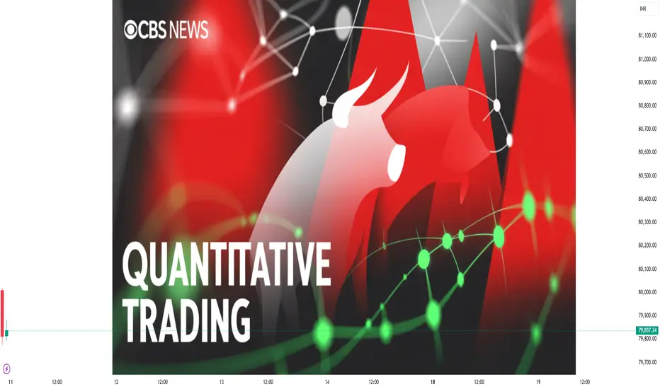
Institutional Trading1. Introduction
Institutional trading refers to the buying and selling of financial securities by large organizations such as banks, pension funds, hedge funds, mutual funds, insurance companies, sovereign wealth funds, and proprietary trading firms. These institutions trade in massive volumes, often involving millions of dollars in a single transaction.
Unlike retail traders, who typically trade through standard brokerage accounts, institutions operate with advanced infrastructure, direct market access, complex strategies, and regulatory privileges that allow them to execute trades with greater efficiency and lower costs.
Institutional traders are not only participants in the market — they shape the market. Their trades can influence prices, liquidity, and even the broader economic sentiment. Understanding how institutional trading works is essential for any serious trader or investor because institutions often set the tone for market trends.
2. Who Are Institutional Traders?
Institutional traders are professionals managing money on behalf of large organizations. Let’s break down the major categories:
a) Hedge Funds
Trade aggressively for profit, often using leverage, derivatives, and high-frequency strategies.
Example: Bridgewater Associates, Citadel, Renaissance Technologies.
They might take both long and short positions, exploiting market inefficiencies.
b) Mutual Funds
Manage pooled investments from retail investors.
Aim for long-term growth, income, or a balanced approach.
Example: Vanguard, Fidelity.
c) Pension Funds
Manage retirement savings for employees.
Focus on stability, long-term returns, and risk management.
Example: CalPERS (California Public Employees' Retirement System).
d) Sovereign Wealth Funds
State-owned investment funds managing surplus reserves.
Example: Norway Government Pension Fund Global, Abu Dhabi Investment Authority.
e) Insurance Companies
Invest premium income in bonds, equities, and other assets.
Require safe, predictable returns to meet policyholder obligations.
f) Investment Banks & Prop Trading Firms
Conduct proprietary trading using their own capital.
Example: Goldman Sachs, JPMorgan Chase.
3. Characteristics of Institutional Trading
Large Trade Sizes
Orders can be worth millions or billions.
Executed in blocks to avoid market disruption.
Sophisticated Strategies
Algorithmic trading, statistical arbitrage, market-making, options strategies.
Access to Better Pricing
Due to volume and relationships with brokers, they get lower commissions and tighter spreads.
Regulatory Framework
Must comply with SEC, SEBI, FCA, or other market regulators.
Have compliance teams to ensure adherence to laws.
Direct Market Access (DMA)
Can place trades directly into exchange order books.
4. How Institutional Trades Differ from Retail Trades
Feature Retail Trading Institutional Trading
Trade Size Small (few thousand USD) Massive (millions to billions)
Execution Through brokers, often at market rates Direct access, negotiated prices
Tools Limited charting, basic platforms Advanced analytics, AI, proprietary systems
Speed Milliseconds to seconds Microseconds to milliseconds
Market Impact Minimal Can move prices significantly
5. How Institutional Orders Are Executed
Because large trades can move prices, institutions often split orders into smaller parts using strategies such as:
a) VWAP (Volume Weighted Average Price)
Executes trades in line with market volume to minimize price impact.
b) TWAP (Time Weighted Average Price)
Spreads execution over a fixed time period.
c) Iceberg Orders
Only a fraction of the total order is visible to the market at any given time.
d) Algorithmic Trading
Automated execution using complex algorithms.
e) Dark Pools
Private exchanges where large orders can be matched without revealing them publicly.
Reduces market impact but has transparency concerns.
6. Institutional Trading Strategies
1. Fundamental Investing
Analyzing company financials, economic indicators, and industry trends.
Example: Pension funds buying blue-chip stocks for decades-long holding.
2. Quantitative Trading
Using mathematical models and statistical analysis.
Example: Renaissance Technologies using predictive algorithms.
3. High-Frequency Trading (HFT)
Microsecond-level trading to exploit tiny price discrepancies.
Requires ultra-low latency systems.
4. Event-Driven Strategies
Trading based on mergers, earnings announcements, political changes.
Example: Merger arbitrage.
5. Sector Rotation
Shifting funds into outperforming sectors.
Often tied to macroeconomic cycles.
6. Smart Money Concepts
Using liquidity, order flow, and price action to anticipate retail moves.
7. Institutional Footprints in the Market
Institutions leave behind clues in the market:
Unusual Volume Spikes – sudden jumps may indicate accumulation or distribution.
Block Trades – large off-market transactions recorded.
Option Flow – heavy institutional positions in specific strikes and expiries.
Retail traders often watch these footprints to follow institutional sentiment.
8. Tools & Technology Used by Institutions
Bloomberg Terminal – real-time data, analytics, and trading execution.
Refinitiv Eikon – market research and analysis.
Custom Trading Algorithms – developed in Python, C++, or Java.
Colocation Services – placing servers next to exchange data centers to minimize latency.
AI & Machine Learning – predictive analytics, sentiment analysis.
9. Advantages Institutions Have
Capital Power – Can hold positions through drawdowns.
Information Access – Analysts, insider corporate access (within legal limits).
Lower Costs – Reduced commissions due to scale.
Execution Speed – Direct market connections.
Market Influence – Ability to move prices in their favor.
10. Risks in Institutional Trading
Liquidity Risk
Large positions are hard to exit without impacting prices.
Counterparty Risk
If trading OTC (over-the-counter), the other party may default.
Regulatory Risk
Sudden rule changes affecting strategies.
Reputational Risk
Large losses can harm public trust (e.g., Archegos Capital collapse).
Systemic Risk
Large institutions failing can trigger market crises (e.g., Lehman Brothers in 2008).
Conclusion
Institutional trading is the backbone of global markets. Institutions have the resources, technology, and strategies to influence prices and liquidity in ways retail traders cannot.
For a retail trader, understanding institutional behavior can provide a significant edge. Watching their footprints — through volume, order flow, filings, and market structure — can help align your trades with the big players rather than against them.
The difference between trading with institutional flows and trading against them can be the difference between consistent profits and constant losses.