Part 8 Trading Master ClassCommon Mistakes to Avoid
Holding OTM options too close to expiry hoping for a miracle.
Selling naked calls without understanding unlimited risk.
Over-leveraging with too many contracts.
Ignoring commissions and slippage.
Not adjusting positions when market changes.
Practical Tips for Success
Backtest strategies on historical data.
Start with paper trading before using real money.
Track your trades in a journal.
Combine technical analysis with options knowledge.
Trade liquid options with tight bid-ask spreads.
X-indicator

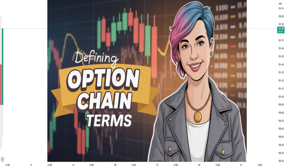
Part11 Trading Master ClassOption Chain Key Terms
Let’s go deep into each term one by one.
Strike Price
The predetermined price at which you can buy (Call) or sell (Put) the underlying asset if you exercise the option.
Every expiry has multiple strike prices — some above the current market price, some below.
Example:
If NIFTY is at 19,500:
19,500 Strike → ATM (At The Money)
19,600 Strike → OTM (Out of The Money) Call, ITM (In The Money) Put
19,400 Strike → ITM Call, OTM Put
Expiry Date
The last trading day for the option. After this date, the contract expires worthless if not exercised.
In India:
Index options (like NIFTY, BANKNIFTY) → Weekly expiries + Monthly expiries
Stock options → Monthly expiries
Call Option (CE)
Gives you the right (not obligation) to buy the underlying at the strike price.
Traders buy calls when they expect the price to rise.
Put Option (PE)
Gives you the right (not obligation) to sell the underlying at the strike price.
Traders buy puts when they expect the price to fall.

Option Chain Terms1. Introduction: What is an Option Chain?
An Option Chain (also called an options matrix) is like a detailed menu for all the available Call and Put options of a particular underlying asset (such as a stock, index, or commodity) for different strike prices and expiry dates.
If you’re a trader, the option chain is where you see all the numbers that decide your trading choices — prices, volumes, open interest, and Greeks.
Think of it as the cockpit of an airplane — lots of data, but if you know what each dial means, you can navigate smoothly.
Example:
If you open the NSE India website and look at the NIFTY Option Chain, you’ll see something like:
Strike Price CALL LTP CALL OI PUT LTP PUT OI
19500 ₹250 1,20,000 ₹15 80,000
19600 ₹180 95,000 ₹25 90,000
This is a simplified snapshot — in reality, there are more columns like bid-ask prices, implied volatility, and Greeks.
2. Core Sections of an Option Chain
An option chain is split into two halves:
Left Side: Call options (bullish contracts)
Right Side: Put options (bearish contracts)
Middle: Strike Prices (common to both)
Here’s how the layout looks visually:
markdown
Copy
Edit
CALL DATA | STRIKE PRICE | PUT DATA
-----------------------------------------------
OI Chg OI LTP IV | 19500 | IV LTP Chg OI OI
OI Chg OI LTP IV | 19600 | IV LTP Chg OI OI
3. Option Chain Key Terms
Let’s go deep into each term one by one.
3.1 Strike Price
The predetermined price at which you can buy (Call) or sell (Put) the underlying asset if you exercise the option.
Every expiry has multiple strike prices — some above the current market price, some below.
Example:
If NIFTY is at 19,500:
19,500 Strike → ATM (At The Money)
19,600 Strike → OTM (Out of The Money) Call, ITM (In The Money) Put
19,400 Strike → ITM Call, OTM Put
3.2 Expiry Date
The last trading day for the option. After this date, the contract expires worthless if not exercised.
In India:
Index options (like NIFTY, BANKNIFTY) → Weekly expiries + Monthly expiries
Stock options → Monthly expiries
3.3 Call Option (CE)
Gives you the right (not obligation) to buy the underlying at the strike price.
Traders buy calls when they expect the price to rise.
3.4 Put Option (PE)
Gives you the right (not obligation) to sell the underlying at the strike price.
Traders buy puts when they expect the price to fall.
3.5 LTP (Last Traded Price)
The most recent price at which the option contract traded.
Reflects the current market value of that option.
3.6 Bid Price & Ask Price
Bid Price: Maximum price buyers are willing to pay.
Ask Price: Minimum price sellers are willing to accept.
The gap between them is called the Bid-Ask Spread.
3.7 Bid Quantity & Ask Quantity
Bid Quantity: Number of contracts buyers want to purchase at the bid price.
Ask Quantity: Number of contracts sellers are offering at the ask price.
3.8 Volume
Total number of contracts traded during the current trading session.
High volume indicates strong interest and liquidity.
3.9 Open Interest (OI)
Total number of outstanding contracts that haven’t been closed or squared off.
Shows market positioning:
High OI in calls → Bearish or range-bound expectation.
High OI in puts → Bullish or range-bound expectation.
3.10 Change in Open Interest (Chg OI)
How much OI has increased or decreased from the previous session.
Used to detect fresh positions or unwinding.
3.11 Implied Volatility (IV)
Market’s expectation of future volatility.
Higher IV → Option premiums become expensive.
Lower IV → Options are cheaper.
3.12 Greeks in the Option Chain
Greeks measure how sensitive the option price is to changes in market factors:
Delta → Price change sensitivity to the underlying asset.
Gamma → Rate of change of Delta.
Theta → Time decay rate of the option price.
Vega → Sensitivity to changes in volatility.
Rho → Sensitivity to interest rate changes.
3.13 ATM, ITM, and OTM
ATM (At The Money): Strike price is equal to the current price.
ITM (In The Money): Option has intrinsic value.
OTM (Out of The Money): Option has no intrinsic value (only time value).
3.14 Premium
The price you pay to buy an option.
Premium = Intrinsic Value + Time Value.
3.15 Break-Even Point
Price level at which your option trade starts becoming profitable.
3.16 PCR (Put-Call Ratio)
Formula: PCR = Put OI / Call OI
High PCR (>1) → Bullish sentiment.
Low PCR (<1) → Bearish sentiment.
4. How to Read the Option Chain
Reading an option chain is about spotting where traders are placing their bets.
Step-by-step:
Identify ATM Strike.
See highest OI in Calls and Puts — this shows resistance and support levels.
Look at Change in OI to spot fresh activity.
Check IV movement for volatility expectations.
Use Greeks for risk assessment.
Example Analysis:
NIFTY at 19,500
Highest Call OI: 19,800 (Resistance)
Highest Put OI: 19,400 (Support)
PCR = 1.2 → Mildly bullish
5. Practical Use Cases
Finding Support & Resistance:
Highest Put OI → Support
Highest Call OI → Resistance
Spotting Breakouts:
Sudden drop in Call OI at resistance → Possible breakout.
Volatility Trading:
High IV → Consider selling options.
Low IV → Consider buying options.
6. Advanced Option Chain Insights
Long Buildup: Price ↑, OI ↑ → Bullish.
Short Buildup: Price ↓, OI ↑ → Bearish.
Short Covering: Price ↑, OI ↓ → Bullish reversal.
Long Unwinding: Price ↓, OI ↓ → Bearish reversal.
7. Common Mistakes to Avoid
Ignoring IV before entering trades.
Reading OI without considering price movement.
Not adjusting for upcoming news or events.
Trading illiquid strikes with wide bid-ask spreads.
8. Conclusion
An option chain is not just a table of numbers — it’s a real-time X-ray of trader sentiment.
By understanding every term — from LTP to IV, from Delta to PCR — you can turn raw data into actionable insights.
Private vs. Public Sector Banks 1. Introduction
Banks are the backbone of any economy. They are not just safe houses for our money; they act as credit suppliers, payment facilitators, and growth enablers for individuals, businesses, and governments.
In India — and in most countries — banks are broadly divided into public sector banks (PSBs) and private sector banks (Pvt banks). While both serve the same core purpose of financial intermediation, their ownership, management, operational style, and even their customer experience differ significantly.
Understanding Private vs. Public Sector Banks is not just an academic exercise — it’s crucial for:
Investors who want to choose where to put their money.
Job seekers deciding between PSU banking careers and private sector opportunities.
Customers looking for the best mix of safety, returns, and service quality.
Policy makers trying to design financial inclusion and credit growth policies.
2. What are Public Sector Banks?
Definition:
A public sector bank is a bank where the majority stake (more than 50%) is held by the government — either the central government, state government, or both.
Key Characteristics:
Ownership: Government-controlled.
Governance: Board of directors often includes government nominees.
Mandate: Balances commercial profitability with social objectives like financial inclusion.
Funding & Support: Can access government capital infusion during crises.
Regulation: Supervised by the Reserve Bank of India (RBI), but also influenced by government policies.
Examples in India:
State Bank of India (SBI) – India’s largest bank.
Punjab National Bank (PNB)
Bank of Baroda (BoB)
Canara Bank
Union Bank of India
Globally, similar examples exist — such as Bank of China or Royal Bank of Scotland (in the past).
3. What are Private Sector Banks?
Definition:
A private sector bank is owned and operated by private individuals or corporations, where the majority of shares are held by private stakeholders.
Key Characteristics:
Ownership: Private promoters and institutional investors.
Governance: Professional boards, often with market-driven incentives.
Mandate: Primarily driven by profitability, efficiency, and shareholder returns.
Customer Orientation: More aggressive in marketing, product innovation, and digital adoption.
Regulation: Supervised by the RBI but largely free from direct government operational control.
Examples in India:
HDFC Bank – India’s largest private sector bank.
ICICI Bank
Axis Bank
Kotak Mahindra Bank
Yes Bank
Globally, examples include JPMorgan Chase, HSBC, and Citibank.
4. Historical Context in India
The distinction between public and private banks in India is rooted in policy decisions.
Pre-Nationalisation Era (Before 1969)
Most banks were privately owned, often run by business families.
Credit was concentrated in urban areas; rural India had limited access.
Frequent bank failures occurred due to poor regulation.
Nationalisation (1969 & 1980)
In 1969, Prime Minister Indira Gandhi nationalised 14 major private banks.
In 1980, 6 more banks were nationalised.
Goal: Direct credit to agriculture, small industries, and backward areas.
Result: PSBs became dominant — controlling over 90% of banking business.
Post-Liberalisation (1991 onwards)
New private banks like HDFC Bank, ICICI Bank, and Axis Bank emerged.
RBI allowed foreign banks to operate more freely.
PSB dominance declined, but they still remain vital for rural outreach.
5. Ownership & Governance Differences
Feature Public Sector Banks Private Sector Banks
Ownership Majority (>50%) by Government Majority by private individuals/institutions
Board Control Government nominees, political influence possible Independent/professional management
Capital Infusion Often from government budget Raised from private investors or markets
Accountability Parliament, RBI, and public scrutiny Shareholders and RBI
6. Objectives & Mandates
Public Sector Banks:
Financial inclusion
Support for agriculture, MSMEs, and infrastructure
Government welfare scheme implementation (e.g., Jan Dhan Yojana)
Stability in rural credit supply
Private Sector Banks:
Profitability and market share growth
Product innovation and niche targeting
Maximizing shareholder returns
Efficiency and cost optimization
7. Operational Style & Customer Service
Public Sector Banks:
Tend to have larger rural branch networks.
Service quality can vary; bureaucratic processes are common.
Product range is adequate but less aggressive in innovation.
Loan approvals may be slower due to multiple verification layers.
Examples: SBI’s YONO app shows digital adaptation, but rollout is slower.
Private Sector Banks:
More urban-centric (though expanding into semi-urban and rural).
Aggressive in customer acquisition and cross-selling.
Loan approvals and service delivery are often faster.
Early adopters of technology — e.g., HDFC Bank’s mobile banking, ICICI’s iMobile app.
More flexible in product design.
8. Technology Adoption
Aspect Public Sector Banks Private Sector Banks
Digital Banking Gradual adoption; integration with legacy systems slows pace Rapid adoption; cloud & AI-powered tools
Customer Onboarding Often in-branch, with KYC paperwork Instant account opening via apps
Innovation Moderate; often after private sector pioneers Aggressive; lead in UPI, API banking
Example: HDFC Bank was among the first in India to launch a net banking platform in 1999. PSBs followed years later.
9. Financial Performance & Profitability
Private banks generally outperform PSBs in:
Return on Assets (RoA)
Return on Equity (RoE)
Net Interest Margin (NIM)
PSBs, however, have:
Larger deposit base due to government trust factor.
Wider financial inclusion footprint.
Example (FY24 Data, approx.):
HDFC Bank RoA: ~2.0%
SBI RoA: ~0.9%
HDFC Bank NIM: ~4.1%
SBI NIM: ~3.2%
10. Risk & NPA Levels
Public Sector Banks:
Historically higher Non-Performing Assets (NPAs) due to priority sector lending, political interference, and legacy loans.
Government recapitalises them when losses mount.
Private Sector Banks:
More selective in lending.
Lower NPA ratios on average.
But risk exists — e.g., Yes Bank crisis in 2020.
11. Role in the Economy
Public Sector Banks:
Act as financial shock absorbers.
Support government borrowing and welfare distribution.
Primary channel for rural development finance.
Private Sector Banks:
Drive innovation in payments, digital finance, and wealth management.
Cater to affluent and corporate clients more aggressively.
Attract foreign investment in India’s banking sector.
12. Global Comparisons
In countries like China, public banks dominate (e.g., Industrial and Commercial Bank of China).
In the US, most banks are privately owned, with government stepping in during crises (e.g., 2008 bailout).
India’s model is hybrid — both sectors coexist, serving different but overlapping needs.
Conclusion
The Public vs. Private Sector Bank debate is not about which is “better” in an absolute sense — both are indispensable pillars of the financial system.
Public sector banks ensure financial inclusion, rural development, and stability, while private sector banks drive efficiency, innovation, and competitive service.
For customers, the best choice often depends on priorities:
If trust, safety, and rural access are key — PSBs shine.
If speed, digital ease, and product innovation matter — private banks lead.
For the economy, a balanced dual banking ecosystem ensures stability and progress.

Mastering the Art of Risk Management in Trading 1. Introduction: Why Risk Management is the Heart of Trading
Trading is not about making big profits quickly — it’s about staying in the game long enough to let your edge work for you.
Think of trading like a professional sport. Skill matters, but survival matters more. Even the world’s best traders lose trades; what separates them from amateurs is how they manage those losses.
In simple terms:
Good trading without risk management = gambling.
Average trading with strong risk management = long-term success.
Warren Buffett’s famous rules apply perfectly here:
Don’t lose money.
Never forget rule #1.
2. Core Principles of Risk Management
Before we go deep into strategies, let’s lock in the foundation.
2.1 Risk is Inevitable
Every trade carries risk. The goal is not to avoid it but to control its size and impact.
2.2 Asymmetry in Trading
A 50% loss requires a 100% gain to break even. This means avoiding large drawdowns is far more important than chasing big wins.
Loss % Required Gain to Recover
10% 11.1%
25% 33.3%
50% 100%
75% 300%
2.3 Risk per Trade
Most professional traders risk 0.5%–2% of their account per trade.
This ensures no single bad trade can destroy the account.
3. The Psychology of Risk
Risk management is not just math — it’s deeply psychological.
Loss Aversion Bias: Humans feel losses twice as strongly as gains. This can push traders into revenge trading.
Overconfidence Bias: Winning streaks can lead to oversized positions.
Fear of Missing Out (FOMO): Chasing trades without proper entry rules increases risk.
A great risk management system removes emotional decision-making by setting clear, mechanical rules.
4. Position Sizing: The Risk Control Lever
Position sizing determines how much capital to put into a trade. Even if your strategy is perfect, bad sizing can blow up your account.
4.1 Fixed Fractional Method
Risk a fixed % of capital per trade.
Example: If account = ₹10,00,000 and risk = 1% → Risk per trade = ₹10,000.
If Stop Loss = ₹50 away from entry, position size = ₹10,000 ÷ ₹50 = 200 shares.
4.2 Volatility-Based Position Sizing
Adjust position size according to the volatility of the asset (ATR – Average True Range).
If ATR = ₹25 and your risk budget = ₹5,000, position size = ₹5,000 ÷ ₹25 = 200 shares.
4.3 Kelly Criterion (Advanced)
Maximizes capital growth based on win rate & reward/risk ratio.
Formula: K% = W – (1 – W) / R
Where:
W = Win probability
R = Reward/Risk ratio
Caution: Kelly is aggressive; use fractional Kelly for real trading.
5. Stop Loss Strategies: Your Safety Net
A stop loss is not a sign of weakness — it’s a shield.
5.1 Fixed Stop Loss
Predefined point in price where you exit.
5.2 Volatility Stop Loss
Adjust stop distance using ATR to account for market noise.
5.3 Time-Based Stop
Exit after a fixed time if the trade hasn’t moved in your favor.
5.4 Trailing Stop
Moves with price in your favor to lock in profits.
Golden Rule: Place stops based on market structure, not emotions.
6. Reward-to-Risk Ratio (RRR)
The RRR tells you how much you stand to gain for every unit you risk.
Example:
Risk: ₹1000
Reward: ₹3000
RRR = 3:1 → Even a 40% win rate is profitable.
High RRR trades allow more losers than winners while staying profitable.
7. Diversification & Correlation Risk
7.1 Asset Diversification
Avoid putting all capital into one asset or sector.
7.2 Correlation Risk
If you buy Nifty futures and Bank Nifty futures, you’re effectively doubling your risk because they move together.
8. Risk Management for Different Trading Styles
8.1 Day Trading
Keep daily loss limits (e.g., 3% of capital).
Avoid revenge trading after a loss.
8.2 Swing Trading
Use wider stops to allow for multi-day fluctuations.
Position sizing becomes even more critical.
8.3 Options Trading
Risk can be higher due to leverage.
Always calculate max loss before entering.
9. Risk Management Tools
ATR Indicator – For volatility-based stops.
Position Size Calculators – To control exposure.
Heat Maps & Correlation Tools – To avoid overexposure.
Journaling Software – To track mistakes.
10. Risk-Adjusted Performance Metrics
Professional traders measure performance relative to risk taken.
Sharpe Ratio – Risk-adjusted returns.
Sortino Ratio – Focuses on downside volatility.
Max Drawdown – Largest account drop during a period.
11. Building a Personal Risk Management Plan
Your plan should cover:
Max % of capital risked per trade.
Max daily/weekly loss limit.
Position sizing rules.
Stop loss & target placement method.
Diversification guidelines.
Rules for scaling in/out.
Plan for handling drawdowns.
12. Advanced Concepts
12.1 Portfolio Heat
Sum of all open trade risks; keep it below a set % of account.
12.2 Value at Risk (VaR)
Estimates the max expected loss over a time frame.
12.3 Stress Testing
Simulate worst-case scenarios (e.g., gap downs, black swans).
Conclusion: Risk Management is Your Superpower
In trading, capital is ammunition. Risk management ensures you never run out of bullets before the big opportunities arrive.
Mastering it is not optional — it’s the difference between a short-lived hobby and a long-term career.
Technical Analysis Concepts1. Introduction to Technical Analysis
Technical Analysis (TA) is the study of market price action—primarily through charts—to forecast future price movements.
It’s built on the idea that “Price discounts everything”, meaning that all known information—economic data, company performance, market sentiment—is already reflected in the price.
In simpler words:
If you want to know what’s happening in a market, don’t just listen to the news—look at the chart.
Key Principles of Technical Analysis
There are three main pillars:
Price Discounts Everything
Every fundamental factor—earnings, interest rates, political events—is already reflected in price.
Traders believe price moves because of demand and supply changes that show up on charts before news does.
Price Moves in Trends
Markets rarely move in random zig-zags—they tend to trend:
Uptrend: Higher highs and higher lows
Downtrend: Lower highs and lower lows
Sideways: No clear direction
History Tends to Repeat Itself
Human psychology—fear, greed, hope—hasn’t changed over centuries. Chart patterns that worked 50 years ago often still work today.
2. Types of Technical Analysis
Broadly, TA can be split into:
A. Chart Analysis (Price Action)
Patterns, trendlines, support, resistance
Focuses purely on price movements
B. Indicator-Based Analysis
Uses mathematical formulas applied to price/volume
Examples: RSI, MACD, Moving Averages
C. Volume Analysis
Studies how much activity supports a price move
Strong moves with high volume = higher reliability
D. Market Structure Analysis
Understanding swing highs/lows, liquidity zones, and institutional footprints
3. Charts and Timeframes
Technical analysis starts with a chart. There are different chart types:
Line Chart – Simplest, connects closing prices. Good for a big-picture view.
Bar Chart – Shows open, high, low, close (OHLC).
Candlestick Chart – The most popular, visually intuitive for traders.
Timeframes
Choosing the right timeframe depends on your trading style:
Scalpers: 1-min to 5-min charts
Intraday Traders: 5-min to 15-min
Swing Traders: 1-hour to daily
Position Traders/Investors: Weekly to monthly
Rule of thumb:
Higher timeframes = stronger signals, but slower trades.
Lower timeframes = faster signals, but more noise.
4. Trends and Trendlines
A trend is simply the market’s general direction.
Types of Trends
Uptrend → Higher highs, higher lows
Downtrend → Lower highs, lower lows
Sideways (Range-bound) → Price moves within a horizontal band
Trendlines
A trendline is drawn by connecting at least two significant highs or lows.
In an uptrend: Connect swing lows
In a downtrend: Connect swing highs
They act as dynamic support or resistance.
5. Support and Resistance
Support: A price level where buying pressure is strong enough to halt a downtrend.
Resistance: A price level where selling pressure stops an uptrend.
How They Work
Support → Demand > Supply → Price bounces
Resistance → Supply > Demand → Price drops
Pro Tip: Once broken, support often becomes resistance and vice versa—this is called role reversal.
6. Chart Patterns
Chart patterns are visual formations on a chart that indicate potential market moves.
A. Continuation Patterns (Trend likely to continue)
Flags – Short pauses after sharp moves
Pennants – Small symmetrical triangles
Rectangles – Price consolidates between parallel support/resistance
B. Reversal Patterns (Trend likely to change)
Head and Shoulders – Signals a bearish reversal
Double Top/Bottom – Two failed attempts to break a high/low
Triple Top/Bottom – Similar to double but with three attempts
C. Bilateral Patterns (Either direction possible)
Triangles – Symmetrical, ascending, descending
7. Candlestick Patterns
Candlestick patterns are short-term signals of buying or selling pressure.
Bullish Patterns
Hammer – Long lower shadow, small body
Bullish Engulfing – Large bullish candle covers previous bearish candle
Morning Star – Three-candle reversal pattern
Bearish Patterns
Shooting Star – Long upper shadow
Bearish Engulfing – Large bearish candle covers prior bullish candle
Evening Star – Three-candle bearish reversal
8. Technical Indicators
Indicators help confirm price action or generate signals.
A. Trend Indicators
Moving Averages (SMA, EMA)
MACD – Measures momentum and trend changes
Parabolic SAR – Trailing stop tool
B. Momentum Indicators
RSI – Overbought (>70) / Oversold (<30) conditions
Stochastic Oscillator – Compares closing price to price range
CCI – Commodity Channel Index for momentum shifts
C. Volatility Indicators
Bollinger Bands – Show price deviation from average
ATR (Average True Range) – Measures volatility strength
D. Volume Indicators
OBV (On-Balance Volume) – Volume flow analysis
VWAP – Volume-weighted average price, used by institutions
9. Volume Profile and Market Structure
Volume Profile shows how much trading occurred at each price level, not just over time.
It highlights:
High Volume Nodes (HVN) → Strong price acceptance
Low Volume Nodes (LVN) → Price rejection zones
Market Structure is about identifying:
Higher highs / higher lows (uptrend)
Lower highs / lower lows (downtrend)
Liquidity pools (where stops are likely)
10. Dow Theory
Dow Theory is the grandfather of trend analysis.
Its principles:
Market discounts everything.
Market has three trends: Primary, secondary, minor.
Trends have three phases: Accumulation, public participation, distribution.
A trend is valid until a clear reversal occurs.
Conclusion
Technical analysis is not about predicting the future with 100% accuracy—it’s about improving probabilities.
A good TA trader:
Understands trends and patterns
Combines multiple tools for confirmation
Manages risk and keeps emotions in check
Remember:
TA gives you the edge, risk management keeps you in the game.

High-Quality Dip Buying1. Introduction – The Essence of Dip Buying
The phrase “Buy the dip” is one of the most common in financial markets — from Wall Street veterans to retail traders on social media. The core idea is simple:
When an asset’s price temporarily falls within an overall uptrend, smart traders buy at that lower price, expecting it to recover and make new highs.
But here’s the reality — not all dips are worth buying. Many traders rush in too soon, only to see the price fall further.
This is why High-Quality Dip Buying is different — it’s about buying dips with probability, timing, and market structure on your side, not just reacting to a red candle.
The goal here is strategic patience, technical confirmation, and risk-controlled execution.
2. Why Dip Buying Works (When Done Right)
Dip buying works because:
Trend Continuation – In a strong uptrend, pullbacks are natural pauses before the next leg higher.
Liquidity Pockets – Price often dips into zones where big players add positions.
Psychological Discounts – Market participants love “getting in at a better price,” creating buying pressure after a drop.
Mean Reversion – Markets often revert to an average after short-term overreactions.
But — without confirming the quality of the dip, traders risk catching a falling knife (a price that keeps dropping without support).
3. What Makes a “High-Quality” Dip?
A dip becomes high quality when:
It occurs in a strong underlying trend (measured with moving averages, higher highs/higher lows, or macro fundamentals).
The pullback is controlled, not panic-driven.
Volume behavior confirms accumulation — volume dries up during the dip and increases on recovery.
It tests a well-defined support zone (key levels, VWAP, 50-day MA, Fibonacci retracement, etc.).
Market sentiment remains bullish despite short-term weakness.
Macro or fundamental story stays intact — no major negative catalyst.
Think of it this way:
A low-quality dip is like buying a “discounted” product that’s broken.
A high-quality dip is like buying a brand-new iPhone during a holiday sale — same product, better price.
4. The Psychology Behind Dip Buying
Understanding trader psychology is critical.
Fear – When prices drop, many panic-sell. This creates opportunities for disciplined traders.
Greed – Some traders jump in too early without confirmation, leading to losses.
Patience – High-quality dip buyers wait for confirmation instead of guessing the bottom.
Confidence – They trust the trend and their plan, avoiding emotional exits.
In other words, dip buying rewards those who stay calm when others are reacting impulsively.
5. Market Conditions Where Dip Buying Thrives
High-quality dip buying works best in:
Strong Bull Markets – Indices and leading sectors are making higher highs.
Post-Correction Recoveries – Markets regain bullish momentum after a healthy pullback.
High-Liquidity Stocks/Assets – Blue chips, large caps, index ETFs, or top cryptos.
Clear Sector Leadership – Strong sectors (tech, healthcare, renewable energy) attract consistent dip buyers.
It’s risky in:
Bear markets (dips often turn into bigger drops)
Illiquid assets (wild volatility without strong support)
News-driven selloffs (fundamental damage)
6. Technical Tools for Identifying High-Quality Dips
A good dip buyer uses price action + indicators + volume.
a) Moving Averages
20 EMA / 50 EMA – Short to medium-term trend guides.
200 SMA – Long-term institutional trend.
High-quality dips often bounce near the 20 EMA in strong trends or the 50 EMA in moderate ones.
b) Support and Resistance Zones
Look for price retracing to:
Previous breakout levels
Trendline support
Volume profile high-volume nodes
c) Fibonacci Retracements
Common dip zones:
38.2% retracement – Healthy shallow pullback.
50% retracement – Neutral zone.
61.8% retracement – Deeper but often still bullish.
d) RSI (Relative Strength Index)
Strong trends often dip to RSI 40–50 before bouncing.
Avoid dips where RSI breaks below 30 and stays weak.
e) Volume Profile
Healthy dips = declining volume during pullback, rising volume on recovery.
7. Step-by-Step: Executing a High-Quality Dip Buy
Here’s a simple process:
Step 1 – Identify the Trend
Use moving averages and price structure (higher highs & higher lows).
Step 2 – Wait for the Pullback
Let price retrace to a strong support area.
Avoid chasing — patience is key.
Step 3 – Look for Confirmation
Reversal candlestick patterns (hammer, bullish engulfing).
Positive divergence in RSI/MACD.
Bounce on increased volume.
Step 4 – Plan Your Entry
Scale in: Start with partial size at the support, add on confirmation.
Use limit orders at planned levels.
Step 5 – Set Stop Loss
Place below recent swing low or key support.
Step 6 – Manage the Trade
Trail stop as price moves in your favor.
Take partial profits at predefined levels.
8. Risk Management in Dip Buying
Even high-quality dips can fail. Protect yourself by:
Never going all-in — scale in.
Using stop losses — don’t hold if structure breaks.
Sizing based on volatility — smaller size for volatile assets.
Limiting trades — avoid overtrading every dip.
9. Real Market Examples
Example 1 – Stock Market
Apple (AAPL) in a bull market often pulls back to the 20 EMA before continuing higher. Traders buying these dips with confirmation have historically seen strong returns.
Example 2 – Cryptocurrency
Bitcoin in a strong uptrend (2020–2021) had multiple 15–20% dips to the 50-day MA — each becoming an opportunity before making new highs.
Example 3 – Index ETFs
SPY ETF during 2019–2021 often dipped to the 50 EMA before strong rallies.
10. Common Mistakes in Dip Buying
Catching a falling knife — Buying without confirmation.
Ignoring news events — Buying into negative fundamental shifts.
Overleveraging — Increasing risk on a guess.
Buying every dip — Not all dips are equal.
No exit plan — Holding losers too long.
Conclusion
High-quality dip buying isn’t about impulsively buying when prices drop. It’s a disciplined, structured, and patient approach that aligns trend, technical analysis, and psychology.
When executed with precision and risk management, it allows traders to buy strength at a discount and participate in powerful trend continuations.
The golden rule?
Never buy a dip just because it’s lower — buy because the trend, structure, and confirmation all align.
RSI Reversal Strategy 1. Introduction to RSI and Why Reversals Matter
In the world of trading, trends are exciting, but reversals are where many traders find their “gold mines.”
Why? Because reversals can catch market turning points before a new trend develops, giving you maximum profit potential from the very start of the move.
One of the most widely used tools to spot these turning points is the Relative Strength Index (RSI). Developed by J. Welles Wilder in 1978, the RSI measures the speed and magnitude of recent price changes to determine whether an asset is overbought or oversold.
In simple words:
RSI tells you when prices have gone too far, too fast, and may be ready to reverse.
It’s like a “market pressure gauge” — too much pressure on one side, and the price often snaps back.
The RSI Reversal Strategy uses these extreme readings to anticipate when a price trend is likely to stall and reverse direction.
2. The RSI Formula (for those who like the math)
While you don’t need to calculate RSI manually in modern charting platforms, it’s important to understand what’s going on under the hood:
𝑅
𝑆
𝐼
=
100
−
(
100
1
+
𝑅
𝑆
)
RSI=100−(
1+RS
100
)
Where:
RS = Average Gain over N periods ÷ Average Loss over N periods
N = The lookback period (commonly 14)
Interpretation:
RSI ranges from 0 to 100
Traditionally:
Above 70 = Overbought
Below 30 = Oversold
Extreme reversals are often spotted above 80 or below 20.
3. Why RSI Works for Reversals
Price movement isn’t random chaos — it’s driven by human behavior: fear, greed, panic, and FOMO.
When price rises too quickly, buyers eventually run out of fuel.
When price drops too sharply, sellers get exhausted.
The RSI measures momentum — and momentum always slows down before a reversal.
The RSI reversal logic is basically saying: “If this much buying or selling pressure was unsustainable before, it’s probably unsustainable now.”
4. Types of RSI Reversal Setups
There are several patterns you can use with RSI to detect reversals. Let’s go step-by-step.
4.1 Classic Overbought/Oversold Reversal
Idea:
When RSI > 70 (or 80), the asset may be overbought → look for short opportunities.
When RSI < 30 (or 20), the asset may be oversold → look for long opportunities.
Example Logic:
RSI crosses above 70 → wait for it to fall back below 70 → enter short.
RSI crosses below 30 → wait for it to climb back above 30 → enter long.
Pros: Very simple, beginner-friendly.
Cons: Works better in ranging markets, can fail in strong trends.
4.2 RSI Divergence Reversal
Idea:
Price makes a new high, but RSI fails to make a new high — or vice versa.
This signals that momentum is weakening, even though price hasn’t reversed yet.
Types:
Bearish Divergence: Price forms higher highs, RSI forms lower highs → possible top.
Bullish Divergence: Price forms lower lows, RSI forms higher lows → possible bottom.
Why it works: Divergence shows that momentum is not supporting the current price movement — a common pre-reversal sign.
4.3 RSI Failure Swing
Idea:
An RSI reversal where the indicator attempts to re-test an extreme level but fails.
Bullish Failure Swing:
RSI drops below 30 (oversold)
RSI rises above 30, then drops again but stays above 30
RSI then breaks the previous high → bullish signal
Bearish Failure Swing:
RSI rises above 70 (overbought)
RSI drops below 70, then rises again but stays below 70
RSI then breaks the previous low → bearish signal
4.4 RSI Reversal Zone Strategy
Idea:
Instead of only looking at 30/70, use custom zones like 20/80 or 25/75 to filter out false signals in trending markets.
5. Timeframes and Market Suitability
RSI works in all markets — stocks, forex, crypto, commodities — but the effectiveness changes with the timeframe.
Scalping/Intraday: 1-min, 5-min, 15-min → RSI 7 or RSI 14 with tighter zones (20/80)
Swing Trading: 1H, 4H, Daily → RSI 14 standard settings
Position Trading: Daily, Weekly → RSI 14 or 21 for smoother signals
Tip:
Shorter timeframes = more signals, but more noise.
Longer timeframes = fewer signals, but stronger reliability.
6. Complete RSI Reversal Strategy Rules (Basic Version)
Let’s build a straightforward rule set.
Parameters:
RSI period: 14
Zones: 30 (oversold), 70 (overbought)
Buy Setup:
RSI drops below 30
RSI rises back above 30
Confirm with price action (e.g., bullish engulfing candle)
Stop-loss below recent swing low
Take profit at 1:2 risk-reward or when RSI nears 70
Sell Setup:
RSI rises above 70
RSI drops back below 70
Confirm with price action (e.g., bearish engulfing candle)
Stop-loss above recent swing high
Take profit at 1:2 risk-reward or when RSI nears 30
7. Advanced RSI Reversal Strategy Enhancements
A pure RSI reversal system can be prone to false signals, especially during strong trends. Here’s how to improve it:
7.1 Combine with Support & Resistance
Only take RSI oversold longs near a support zone.
Only take RSI overbought shorts near a resistance zone.
7.2 Add Volume Confirmation
Look for volume spikes or unusual activity when RSI hits reversal zones — stronger reversal probability.
7.3 Use Multiple Timeframe Confirmation
If you see an RSI reversal on a 15-min chart, check the 1H chart.
When both timeframes align, the reversal is more likely to work.
7.4 Combine with Candlestick Patterns
Reversal candlestick patterns like:
Hammer / Inverted Hammer
Doji
Engulfing
Morning/Evening Star
… can make RSI signals much more reliable.
7.5 RSI Trendline Breaks
Draw trendlines directly on RSI. If RSI breaks its own trendline, it can signal an early reversal before price follows.
8. Risk Management for RSI Reversal Trading
Even the best reversal setups fail sometimes — especially in strong trends where RSI can stay overbought or oversold for a long time.
Golden Rules:
Never risk more than 1–2% of your capital on a single trade.
Always place a stop-loss — don’t assume the reversal will happen immediately.
Use a risk-reward ratio of at least 1:2.
Avoid revenge trading after a loss — overtrading is the #1 account killer.
9. Example Trade Walkthrough
Let’s go through a bullish RSI reversal trade on a stock.
Market: Reliance Industries (Daily chart)
Observation: RSI drops to 22 (extremely oversold) while price nears a major support level from last year.
Trigger: RSI crosses back above 30 with a bullish engulfing candle on the daily chart.
Entry: ₹2,350
Stop-loss: ₹2,280 (below swing low)
Target: ₹2,500 (risk-reward ~1:2)
Result: Price rallies to ₹2,520 in 7 trading days.
10. Common Mistakes to Avoid
Using RSI blindly without price action
RSI needs context — never enter just because it’s overbought or oversold.
Trading against strong trends
RSI can stay extreme for a long time; wait for price action confirmation.
Too small timeframes for beginners
Lower timeframes have too much noise — start with daily/4H charts.
Ignoring market news
Fundamental events can invalidate technical signals instantly.
Conclusion
The RSI Reversal Strategy is powerful because it taps into one of the most consistent behaviors in the market — momentum exhaustion.
When applied with proper filters like support/resistance, candlestick confirmation, and disciplined risk management, it can become a high-probability trading edge.
However — and this is key — no strategy is bulletproof. The RSI Reversal Strategy will fail sometimes, especially in parabolic moves or during strong news-driven trends. Your long-term success depends on how well you manage risk and filter bad signals.
Think of RSI as your early warning radar, not an autopilot. Let it tell you when to pay attention, then confirm with your trading plan before taking action.
Part6 Learn Institution TradingIntroduction to Options Trading
Options are like a financial “contract” that gives you rights but not obligations.
When you buy an option, you are buying the right to buy or sell an asset at a specific price before a certain date.
They’re mainly used in stocks, commodities, indexes, and currencies.
Two main types of options:
Call Option – Right to buy an asset at a set price.
Put Option – Right to sell an asset at a set price.
Key terms:
Strike Price – The price at which you can buy/sell the asset.
Expiration Date – The last day you can use the option.
Premium – Price paid to buy the option.
In the Money (ITM) – Option has intrinsic value.
Out of the Money (OTM) – Option has no intrinsic value yet.
At the Money (ATM) – Strike price equals current market price.
Options give traders flexibility, leverage, and hedging power. But with great power comes great “margin calls” if you misuse them.
Why Traders Use Options
Options aren’t just for speculation — they have multiple uses:
Speculation – Betting on price moves.
Hedging – Protecting an existing investment from loss.
Income Generation – Selling options for premium income.
Risk Management – Limiting losses through defined-risk trades.

Part7 Trading Master ClassPractical Tips for Success
Backtest strategies on historical data.
Start with paper trading before using real money.
Track your trades in a journal.
Combine technical analysis with options knowledge.
Trade liquid options with tight bid-ask spreads.
Final Thoughts
Options are like a Swiss Army knife in trading — versatile, powerful, and potentially dangerous if misused. The right strategy depends on:
Market view (up, down, sideways, volatile, stable)
Risk tolerance
Timeframe
Experience level
By starting with basic strategies like covered calls or protective puts, then moving into spreads, straddles, and condors, you can build a strong foundation. With practice, risk management, and discipline, options trading can be a valuable tool in your investment journey.

Part1 Ride The Big MovesUnderstanding Greeks (The DNA of Options Pricing)
Delta – How much the option price changes per ₹1 move in stock.
Gamma – How fast delta changes.
Theta – Time decay rate.
Vega – Sensitivity to volatility changes.
Rho – Interest rate sensitivity.
Mastering the Greeks means you understand why your option is moving, not just that it’s moving.
Common Mistakes to Avoid
Holding OTM options too close to expiry hoping for a miracle.
Selling naked calls without understanding unlimited risk.
Over-leveraging with too many contracts.
Ignoring commissions and slippage.
Not adjusting positions when market changes.

Part4 Institutional TradingStraddle
When to Use: Expect big move but unsure direction.
How It Works: Buy call and put at same strike & expiry.
Risk: High premium cost.
Reward: Big if price moves sharply up or down.
Example: Stock at ₹100, buy call ₹100 (₹4) and put ₹100 (₹4). Cost ₹8. Needs a big move to profit.
Strangle
When to Use: Expect big move but want cheaper entry than straddle.
How It Works: Buy OTM call and put.
Risk: Cheaper than straddle but needs larger move.
Example: Stock at ₹100, buy call ₹105 (₹3) and put ₹95 (₹3). Cost ₹6.
Iron Condor
When to Use: Expect low volatility.
How It Works: Sell an OTM call spread + sell an OTM put spread.
Risk: Limited by spread width.
Reward: Limited to premium collected.
Example: Stock at ₹100, sell call ₹110, buy call ₹115; sell put ₹90, buy put ₹85.

Part2 Ride The Big Moves Intermediate Options Strategies
Bull Call Spread
When to Use: Expect moderate price rise.
How It Works: Buy a call at a lower strike, sell a call at higher strike.
Risk: Limited to net premium paid.
Reward: Limited to strike difference minus premium.
Example: Buy call at ₹100 (₹5), sell call at ₹110 (₹2). Net cost ₹3. Max profit ₹7.
Bear Put Spread
When to Use: Expect moderate decline.
How It Works: Buy put at higher strike, sell put at lower strike.
Risk: Limited to net premium paid.
Reward: Limited but cheaper than buying a single put.
Example: Buy put ₹105 (₹6), sell put ₹95 (₹3). Net cost ₹3. Max profit ₹7.

Part8 Trading Master ClassIntroduction to Options Trading
Options are like a financial “contract” that gives you rights but not obligations.
When you buy an option, you are buying the right to buy or sell an asset at a specific price before a certain date.
They’re mainly used in stocks, commodities, indexes, and currencies.
Two main types of options:
Call Option – Right to buy an asset at a set price.
Put Option – Right to sell an asset at a set price.
Key terms:
Strike Price – The price at which you can buy/sell the asset.
Expiration Date – The last day you can use the option.
Premium – Price paid to buy the option.
In the Money (ITM) – Option has intrinsic value.
Out of the Money (OTM) – Option has no intrinsic value yet.
At the Money (ATM) – Strike price equals current market price.
Options give traders flexibility, leverage, and hedging power. But with great power comes great “margin calls” if you misuse them.

Psychology & Risk Management in Trading 1. Introduction
Trading is often thought of as a purely numbers-driven game — charts, technical indicators, fundamental analysis, and economic data. But in reality, the true battlefield is inside your head. Two traders can have access to the exact same market data, yet end up with completely different results. The difference lies in psychology and risk management.
Psychology determines how you make decisions under pressure.
Risk management determines whether you survive long enough to benefit from good decisions.
Think of trading as a three-legged stool:
Strategy – Your technical/fundamental system for entering and exiting trades.
Psychology – Your ability to stick to the plan under real conditions.
Risk Management – Your safeguard against catastrophic loss.
If one leg is missing, the stool collapses. A profitable strategy without psychological discipline becomes useless. A strong mindset without proper risk controls eventually faces ruin. And perfect risk management without skill or discipline simply results in slow losses.
Our goal here is to align mindset with money management for long-term success.
2. Understanding Trading Psychology
2.1. Why Psychology Matters More Than You Think
When you’re trading, money is not just numbers — it represents:
Security (fear of losing it)
Freedom (desire to win more)
Ego (feeling smart or dumb based on market outcomes)
This emotional attachment creates mental biases that cloud judgment. Unlike a chessboard, the market is an uncertain game — the same move can lead to a win or loss depending on external forces beyond your control.
The primary enemy is not “the market,” but you:
Closing winning trades too early out of fear.
Holding onto losing trades hoping they’ll recover.
Overtrading to “make back” losses.
Avoiding valid setups after a losing streak.
2.2. The Main Psychological Biases in Trading
1. Loss Aversion
Humans hate losing more than they like winning. Research shows losing $100 feels twice as bad as gaining $100 feels good.
In trading, this causes:
Refusing to take stop losses.
Adding to losing positions to “average down.”
2. Overconfidence Bias
After a streak of wins, traders often overestimate their skill.
Example: Turning a $1,000 account into $2,000 in a week might lead to doubling trade size without a valid reason.
3. Confirmation Bias
Seeking only information that supports your existing view. If you’re bullish on gold, you might only read bullish news and ignore bearish signals.
4. Recency Bias
Giving too much weight to recent events. A trader who just experienced a big rally might expect it to continue, ignoring long-term resistance levels.
5. Fear of Missing Out (FOMO)
Jumping into trades without proper analysis because you see the market moving.
6. Revenge Trading
Trying to “get back” at the market after a loss by taking impulsive trades.
2.3. Emotional States and Their Effects
Fear – Leads to hesitation, missed opportunities, and premature exits.
Greed – Leads to over-leveraging and chasing setups.
Hope – Keeps traders in losing trades far longer than necessary.
Regret – Causes paralysis, stopping you from entering new opportunities.
Euphoria – False sense of invincibility, leading to reckless trades.
3. Mastering the Trader’s Mindset
3.1. Accepting Uncertainty
Markets are probabilistic, not certain. The best trade setups still lose sometimes. The key is to think in terms of probabilities, not certainties.
Mental shift:
Bad trade ≠ losing trade.
Good trade ≠ winning trade.
A “good trade” is one where you followed your plan and managed risk — regardless of the outcome.
3.2. Developing Discipline
Discipline means doing what your trading plan says every time, even when you feel like doing otherwise.
Practical ways to build discipline:
Pre-market checklist (entry/exit rules, risk per trade, market conditions).
Post-trade review to identify emotional decisions.
Simulated trading to practice following rules without monetary pressure.
3.3. Managing Emotional Cycles
Traders often go through repeated emotional phases:
Excitement – New strategy, first wins.
Euphoria – Overconfidence and overtrading.
Fear/Panic – Sharp drawdown after reckless trades.
Desperation – Trying to recover losses quickly.
Resignation – Stepping back, reevaluating.
Rebuilding – Adopting better discipline.
Your goal is to flatten the cycle, reducing extreme highs and lows.
4. Risk Management: The Survival Mechanism
4.1. The Goal of Risk Management
Trading is not about avoiding losses — losses are inevitable. The aim is to control the size of your losses so they don’t destroy your capital or confidence.
4.2. The Three Pillars of Risk Management
1. Position Sizing
Determine how much capital to risk per trade. Common rules:
Risk only 1–2% of total capital on any single trade.
Example: If you have ₹1,00,000 and risk 1% per trade, your max loss is ₹1,000.
2. Stop Losses
Predetermined exit points to limit losses.
Hard stops – Fixed at a price level.
Trailing stops – Move with the trade to lock in profits.
3. Risk-Reward Ratio
A measure of potential reward vs. risk.
Example:
Risk: ₹500
Potential Reward: ₹1,500
R:R = 1:3 (good)
4.3. The Power of Capital Preservation
Here’s why big losses are dangerous:
Lose 10% → Need 11% gain to recover.
Lose 50% → Need 100% gain to recover.
The bigger the loss, the harder the comeback. Capital preservation should be your #1 priority.
4.4. Avoiding Overleveraging
Leverage magnifies both gains and losses. Many traders blow accounts not because their strategy was bad, but because they used excessive leverage.
5. Integrating Psychology with Risk Management
5.1. The Feedback Loop
Poor psychology → Poor risk decisions → Bigger losses → Worse psychology.
You must break the loop by locking in good risk rules before trading.
5.2. The Risk Management Mindset
Treat each trade as just one of thousands you’ll make.
Focus on execution quality, not daily P/L.
Celebrate following your plan, not just winning.
5.3. Journaling
A trading journal should include:
Entry/exit points and reasons.
Risk per trade.
Emotional state before/during/after.
Lessons learned.
Over time, patterns emerge that reveal weaknesses in both mindset and risk control.
6. Practical Tips for Building Psychological Strength
Meditation & Mindfulness – Keeps emotions in check.
Physical Health – A healthy body supports a calm mind.
Sleep – Fatigue increases impulsive decisions.
Routine – Structured trading hours reduce stress.
Detach from P/L – Judge performance over months, not days.
7. Case Studies: When Psychology Meets Risk
Case Study 1 – The Overconfident Scalper
Wins 10 trades in a row, doubles position size.
One loss wipes out previous gains.
Lesson: Stick to fixed risk % per trade regardless of winning streaks.
Case Study 2 – The Hopeful Investor
Holds losing position for months.
Avoids taking stop loss because “it’ll recover.”
Lesson: Hope is not a strategy; use predefined exits.
8. Conclusion
Trading success is 20% strategy and 80% mindset + risk control. The market will always test your patience, discipline, and emotional control. By mastering your psychology and implementing rock-solid risk management, you give yourself the best chance not just to make money — but to stay in the game long enough to grow it.

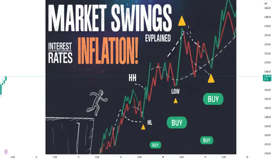
Inflation & Interest Rate Impact on Markets 1. Introduction – Why This Topic Matters
Inflation and interest rates are like the heartbeat and blood pressure of the global economy. When they rise or fall, every financial market — from stocks and bonds to commodities and currencies — reacts. These two forces can determine:
The cost of money (borrowing/lending rates)
The value of assets (how much investors are willing to pay for future earnings)
Consumer spending power (how much people can buy with their money)
Investment flows (where capital moves globally)
Understanding how they interact is crucial for traders, investors, policymakers, and even businesses planning budgets.
2. Understanding Inflation
Inflation is the general rise in prices over time, which reduces the purchasing power of money.
2.1 Types of Inflation
Demand-Pull Inflation
Driven by strong consumer demand outpacing supply.
Example: Post-pandemic reopening in 2021–2022 led to huge spending surges and price hikes.
Cost-Push Inflation
Driven by rising production costs (wages, raw materials, energy).
Example: Oil price spike due to geopolitical tensions.
Built-In Inflation
When workers demand higher wages to keep up with prices, which increases costs for businesses, causing more inflation — the wage-price spiral.
Hyperinflation
Extreme, rapid price increases (often 50%+ per month).
Example: Zimbabwe in the 2000s, Venezuela in the 2010s.
2.2 Measuring Inflation
CPI (Consumer Price Index) — Measures average price change for a basket of goods/services.
PPI (Producer Price Index) — Measures wholesale/production cost changes.
Core Inflation — CPI without volatile food & energy prices (better for long-term trends).
PCE (Personal Consumption Expenditures) — The Fed’s preferred measure in the U.S.
2.3 Causes of Inflation Surges
Supply chain disruptions (COVID-19 impact)
Commodity shocks (oil, metals, food)
Loose monetary policy (low interest rates, money printing)
Fiscal stimulus (government spending boosts demand)
3. Understanding Interest Rates
Interest rates represent the cost of borrowing money, usually set by central banks for short-term lending.
3.1 Types of Rates
Policy Rate
Set by central banks (e.g., U.S. Fed Funds Rate, RBI Repo Rate in India).
Market Rates
Determined by supply/demand in bond markets (long-term yields like the 10-year Treasury).
Real vs. Nominal Rates
Nominal rate = stated rate
Real rate = nominal rate − inflation rate
Example: If interest rate = 5% and inflation = 6%, the real rate is −1% (losing purchasing power).
3.2 Why Central Banks Adjust Rates
To fight inflation — raise rates to cool spending.
To boost growth — cut rates to encourage borrowing.
To stabilize currency — higher rates attract foreign capital, strengthening the currency.
4. The Inflation–Interest Rate Relationship
The two are deeply linked.
High inflation → central banks raise interest rates to slow the economy.
Low inflation or deflation → central banks cut rates to stimulate demand.
This relationship is central to monetary policy.
4.1 The Lag Effect
Interest rate changes take 6–18 months to fully impact inflation and growth. This delay means policymakers act based on forecasts, not current numbers.
4.2 The Risk of Over-Tightening or Under-Tightening
Over-tightening: Raising rates too much can cause recession.
Under-tightening: Keeping rates low for too long can cause runaway inflation.
5. Impact on Financial Markets
5.1 Stock Markets
High Inflation + Rising Rates
Bad for growth stocks (tech, startups) because future earnings are discounted more heavily.
Sectors like utilities, real estate, and consumer discretionary may underperform.
Moderate Inflation + Stable Rates
Can support equities, especially cyclical sectors (industrials, consumer goods).
Low Inflation + Low Rates
Great for growth stocks and speculative investments.
Historical Example:
In 2022, the U.S. Fed hiked rates aggressively to fight 40-year-high inflation. The S&P 500 dropped ~19% for the year, with tech-heavy Nasdaq falling ~33%.
5.2 Bond Markets
When rates rise → bond prices fall (inverse relationship).
Inflation erodes fixed returns from bonds.
TIPS (Treasury Inflation-Protected Securities) outperform during high inflation because they adjust payouts to CPI.
5.3 Currency Markets (Forex)
Higher rates → stronger currency (capital inflows).
Lower rates → weaker currency.
Inflation can weaken a currency if it erodes trust in stability.
Example: The U.S. dollar index (DXY) surged in 2022 due to aggressive Fed hikes.
5.4 Commodities
Inflation often boosts commodity prices (oil, gold, agricultural products).
Gold performs well in high inflation but can underperform when rates rise sharply (due to higher opportunity cost of holding non-yielding assets).
5.5 Real Estate
Higher rates → higher mortgage costs → cooling housing demand.
Inflation in construction materials → higher building costs.
6. Sector-by-Sector Effects
Sector High Inflation Impact High Interest Rate Impact
Technology Negative Very Negative
Energy Positive Neutral to Positive
Consumer Staples Neutral to Positive Neutral
Consumer Discretionary Negative Negative
Financials Positive (loan demand) Positive (better margins)
Real Estate Negative (costs up) Negative (loan cost high)
7. Historical Case Studies
7.1 1970s Stagflation
Inflation above 10%, slow growth, oil shocks.
Fed raised rates to 20% in early 1980s to crush inflation.
Stocks suffered, gold surged.
7.2 2008 Global Financial Crisis
Low inflation but collapsing growth.
Central banks cut rates to near-zero.
Stock markets rebounded post-2009.
7.3 2021–2023 Post-COVID Inflation Surge
Supply chain bottlenecks, stimulus, and energy shocks.
Fed and ECB hiked rates fastest in decades.
Equity valuations compressed, bonds sold off, dollar strengthened.
8. Trading & Investment Strategies
8.1 For High Inflation Environments
Favor real assets (commodities, real estate, infrastructure).
Use inflation-protected bonds.
Short-duration fixed income instead of long bonds.
8.2 For Rising Interest Rates
Reduce exposure to long-duration assets.
Consider value stocks over growth stocks.
Use currency carry trades in favor of higher-rate countries.
8.3 For Falling Rates
Increase equity exposure, especially growth sectors.
Extend bond duration to lock in higher yields before they drop.
Real estate investment can rebound.
9. The Psychology of Markets
Inflation and rate hikes affect sentiment — fear of recession, optimism in easing cycles.
Expectation management by central banks is as important as actual moves.
Markets often price in changes before they happen.
10. Key Takeaways
Inflation and interest rates are interconnected — one drives changes in the other.
Their effects ripple through stocks, bonds, commodities, currencies, and real estate.
Different sectors and asset classes respond differently.
Historical patterns offer guidance but each cycle has unique triggers.
Traders can position based on anticipated shifts rather than reacting late.
Smart Money Concepts1. Introduction: What is Smart Money Concepts?
Smart Money Concepts (SMC) is a modern price action trading methodology that focuses on how big players — institutions, hedge funds, banks, and market makers — move the market.
The core belief: price is manipulated by "smart money" to accumulate positions before large moves, and if you can track their footprints, you can ride their moves instead of getting trapped like retail traders.
In SMC, you don’t rely on indicators that lag behind price. Instead, you learn to read the raw story of price action: where liquidity lies, where stop hunts happen, and where imbalances push price.
Think of it like this:
Retail trading is reacting to price.
SMC trading is predicting what price will want to do, based on smart money’s needs.
2. Core Principles of SMC
SMC builds around a few non-negotiable principles:
2.1 Market Structure
Price moves in waves (higher highs, higher lows in an uptrend, or lower highs, lower lows in a downtrend).
Smart money manipulates these structures:
Break of Structure (BOS): When price breaks a significant swing point in the direction of the trend.
Change of Character (ChoCH): A shift in market bias — often the first sign of trend reversal.
Example:
If we’re in an uptrend and suddenly a major low is broken, this isn’t “random selling.” It’s likely a smart money signal that distribution has started.
2.2 Liquidity
Smart money hunts liquidity pools — areas where retail traders have stop-loss orders:
Above recent highs → stop-losses of short sellers.
Below recent lows → stop-losses of long traders.
Why? Because triggering these stops provides the volume big players need to enter large positions without causing huge slippage.
2.3 Order Blocks
An Order Block is the last opposite candle before a strong impulsive move.
For example:
In an uptrend: the last bearish candle before a strong bullish push.
In a downtrend: the last bullish candle before a strong bearish push.
Order blocks are institutional footprints — zones where smart money likely placed big orders.
2.4 Imbalance & Fair Value Gap (FVG)
Sometimes price moves so fast in one direction that it leaves a gap between candles’ wicks — meaning no trades happened in that range.
Price often revisits these Fair Value Gaps to “rebalance” the market before continuing.
2.5 Premium & Discount Zones
Using Fibonacci retracement, the 50% level divides the market into:
Premium (above 50%) → expensive zone for buying, better for selling.
Discount (below 50%) → cheap zone for buying, better for selling.
Smart money often buys at a discount and sells at a premium.
3. How Smart Money Operates
Retail traders believe price moves randomly — smart money knows better.
3.1 Accumulation & Distribution
Markets cycle through:
Accumulation → Smart money quietly builds positions at low prices.
Manipulation → Stop hunts and fake breakouts to mislead retail traders.
Distribution → Price moves explosively in their intended direction.
3.2 Stop Hunts
Smart money deliberately pushes price to known liquidity areas:
Looks like a breakout to retail traders → but reverses right after.
This traps breakout traders and activates their stops, providing liquidity.
3.3 Inducement
Before moving toward the main liquidity pool, smart money creates a “bait” level to attract retail orders. This induces traders to place stops exactly where smart money wants.
4. SMC Tools & Key Components
4.1 Market Structure Tools
Swing highs/lows
BOS (Break of Structure)
ChoCH (Change of Character)
4.2 Liquidity Identification
Equal highs/lows (double tops/bottoms)
Trendline liquidity (breakouts)
Session highs/lows (London, New York, Asia)
4.3 Order Blocks
Bullish OB → for buys
Bearish OB → for sells
Refined OB → using lower timeframes for precision
4.4 Fair Value Gaps
Look for large impulse moves leaving gaps between candle wicks.
4.5 Fibonacci Levels
Use 50% as a bias divider, 61.8% & 78.6% for sniper entries.
5. The SMC Trading Process
Here’s a step-by-step method to apply SMC:
Step 1: Higher Timeframe Bias
Start from daily (D1) or 4H charts.
Identify market structure (uptrend, downtrend, or range).
Mark major BOS and ChoCH points.
Step 2: Identify Liquidity Pools
Look for equal highs/lows, trendlines, swing points.
Mark where retail traders are likely trapped.
Step 3: Locate Order Blocks
Find the last opposite candle before a strong move.
Confirm it aligns with your higher timeframe bias.
Step 4: Watch for Imbalance
Mark Fair Value Gaps for potential retracements.
Step 5: Entry Execution
Drop to lower timeframes (5M, 1M) for refined entries.
Wait for a lower timeframe BOS in the direction of your trade.
Step 6: Risk Management
Stop-loss just beyond the order block or liquidity sweep point.
Risk 1–2% per trade.
6. Example Trade Setup
Imagine EUR/USD is in an uptrend on 4H:
4H BOS confirmed bullish bias.
Liquidity found below equal lows at 1.0750.
Bullish order block spotted just below 1.0750.
Fair Value Gap in that same area.
On 5M chart → price sweeps liquidity, taps OB, breaks minor high.
Entry after BOS → SL below OB → TP at previous high.
7. SMC vs Traditional Technical Analysis
Aspect Traditional TA SMC
Indicators Uses RSI, MACD, Moving Averages Pure price action
Focus Patterns (Head & Shoulders, etc.) Liquidity, order flow
Timing Often late entries Precision entries
Mindset Follow trend Follow smart money
8. Common Mistakes in SMC Trading
Over-marking charts → clutter leads to confusion.
Forcing trades without waiting for confirmation.
Ignoring higher timeframe bias.
Not managing risk — precision doesn’t mean perfection.
9. Psychology of SMC Trading
SMC can give very high RR trades (1:5, 1:10), but the patience required can be tough.
You need:
Discipline to wait for setups.
Emotional detachment from market noise.
Confidence to enter when it feels counterintuitive.
10. Final Thoughts: Why SMC Works
SMC works because it aligns your trading with the actual drivers of price — the big money.
Instead of being prey, you become a shadow of the predator.
Key takeaways:
Market is a liquidity game.
Learn where smart money is likely to act.
Trade less, but with sniper precision.

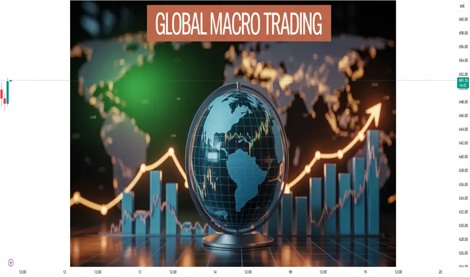
Global Macro Trading1. Introduction to Global Macro Trading
Global macro trading is like playing chess on a planetary board.
Instead of just focusing on a single company or sector, you’re watching how the entire world economy moves—tracking interest rates, currencies, commodities, geopolitical tensions, and policy changes—then placing trades based on your macroeconomic outlook.
At its core:
“Macro” = Large-scale economic factors
Goal = Profit from broad market moves triggered by these factors.
It’s the domain where George Soros famously “broke the Bank of England” in 1992 by shorting the pound, and where hedge funds like Bridgewater use economic cycles to decide positions.
2. The Philosophy Behind Global Macro
The idea is simple: economies move in cycles—boom, slowdown, recession, recovery.
These cycles are driven by:
Interest rates
Inflation & deflation
Government policies
Trade balances
Currency strength/weakness
Geopolitical events
Global macro traders seek to anticipate big shifts—not just day-to-day noise—and bet accordingly.
The moves are often multi-asset: FX, commodities, equities, and bonds all come into play.
3. Key Tools of the Global Macro Trader
Global macro traders don’t just glance at charts—they build a full “global dashboard” of indicators.
A. Economic Data
GDP Growth Rates – Signs of expansion or contraction.
Inflation – CPI, PPI, and core inflation measures.
Employment data – Non-farm payrolls (US), unemployment rates.
Purchasing Managers Index (PMI) – Early signal of economic health.
Consumer Confidence – Sentiment as a leading indicator.
B. Central Bank Policy
Interest Rate Changes – Fed, ECB, BoJ, RBI decisions.
Quantitative Easing/Tightening – Money supply adjustments.
Forward Guidance – Central bank speeches hinting future moves.
C. Market Sentiment
VIX (Volatility Index)
COT (Commitment of Traders) reports
Currency positioning data
D. Geopolitical Risks
Wars, sanctions, trade disputes.
Elections in major economies.
Energy supply disruptions.
4. Core Instruments Used in Global Macro
Global macro traders use multiple asset classes because economic trends ripple across markets.
Currencies (FX) – Betting on relative strength between nations.
Example: Shorting the yen if Japan keeps rates ultra-low while the US hikes.
Government Bonds – Positioning for rising or falling yields.
Example: Buying US Treasuries in risk-off conditions.
Equity Indices – Long or short entire markets.
Example: Shorting the FTSE 100 if UK recession fears rise.
Commodities – Crude oil, gold, copper, agricultural goods.
Example: Long gold during geopolitical instability.
Derivatives – Futures, options, and swaps to hedge or leverage.
5. Styles of Global Macro Trading
Global macro is not one-size-fits-all. Traders pick different timeframes and strategies.
A. Discretionary Macro
Human-driven decision-making.
Uses news, analysis, and gut instinct.
Pros: Flexibility in unusual events.
Cons: Subjective, emotional bias risk.
B. Systematic Macro
Algorithmic, rules-based.
Uses historical correlations, signals.
Pros: Discipline, backtesting possible.
Cons: May miss sudden regime changes.
C. Event-Driven Macro
Trades around specific catalysts.
Examples: Brexit vote, OPEC meeting, US elections.
D. Thematic Macro
Focuses on big themes over months or years.
Example: Betting on long-term dollar weakness due to US debt growth.
6. Fundamental Analysis in Macro
Here’s how a macro trader might think:
Example: US Interest Rates Rise
USD likely strengthens (carry trade appeal).
US Treasuries yields rise → prices fall.
Emerging market currencies weaken (capital flows to USD).
Gold may fall as yield-bearing assets look more attractive.
The chain reaction thinking is key—every macro event has a ripple effect.
7. Technical Analysis in Macro
While fundamentals set the direction, technicals help with timing.
Moving Averages – Identify trend direction.
Breakouts & Support/Resistance – Confirm market shifts.
Fibonacci Levels – Gauge pullback/reversal zones.
Volume Profile – See where major players are active.
Intermarket Correlation Charts – Compare FX, bonds, and commodities.
8. Risk Management in Macro Trading
Macro trades can be big winners—but also big losers—because they often involve leverage.
Key principles:
Never risk more than 1–2% of capital on a single trade.
Diversify across asset classes.
Use stop-loss orders.
Hedge positions (e.g., long oil but short an oil-sensitive currency).
9. Examples of Historical Macro Trades
A. Soros & the Pound (1992)
Bet: UK pound overvalued in the ERM.
Action: Shorted GBP heavily.
Result: £1 billion profit in one day.
B. Paul Tudor Jones & 1987 Crash
Used macro signals to foresee stock market collapse.
Went short S&P 500 futures.
C. Oil Spike 2008
Many traders went long crude as supply fears rose and USD weakened.
10. The Global Macro Trading Process
Macro Research
Economic releases, policy trends, historical cycles.
Hypothesis Building
Example: “If the Fed keeps rates high while ECB cuts, EUR/USD will fall.”
Instrument Selection
Pick the cleanest trade (FX, bonds, commodities).
Position Sizing
Based on risk tolerance and conviction.
Execution & Timing
Use technicals for entry/exit.
Monitoring
Constantly reassess as data comes in.
Exit Strategy
Profit targets and stop-losses in place.
Final Takeaways
Global macro trading is the Formula 1 of financial markets—fast, complex, and requiring mastery of multiple disciplines.
Success depends on:
Staying informed.
Thinking in cause-and-effect chains.
Managing risk religiously.
Being adaptable to changing regimes.
A disciplined global macro trader can profit in bull markets, bear markets, and everything in between—because they’re not tied to one asset or region.
Instead, they follow the money and the momentum wherever it flows.
Volume Profile & Market Structure Analysis1. Introduction
If you’ve been trading for a while, you’ve probably noticed something: prices don’t move randomly. They dance around certain areas, stall at specific levels, and reverse at others. That’s no coincidence. It’s market structure at play — the way price organizes itself — and volume profile helps us see where the market cares most.
Think of market structure as the skeleton of price action and volume profile as the X-ray showing where the “meat” (volume) is attached. Together, they can give traders a huge edge in understanding the battlefield between buyers and sellers.
2. The Basics of Volume Profile
2.1 What Is Volume Profile?
Volume Profile is a charting tool that plots the amount of trading volume at each price level over a chosen time period. Instead of showing volume below the chart (like a regular volume histogram), it plots it horizontally along the price axis.
It tells you:
Where the most trading activity happened (high volume nodes)
Where little activity happened (low volume nodes)
Which price levels acted as magnets or barriers for price
Key Components:
Point of Control (POC): The price level where the most volume traded.
Value Area (VA): The range of prices where ~70% of the total volume occurred (Value Area High = VAH, Value Area Low = VAL).
High Volume Nodes (HVN): Price levels with heavy trading interest.
Low Volume Nodes (LVN): Price levels with minimal trading activity.
2.2 Why Volume Profile Matters
Shows Market Consensus: Prices with high volume indicate agreement between buyers and sellers — they’re comfortable transacting there.
Identifies Support/Resistance: HVNs often act like magnets, LVNs often act like rejection zones.
Helps Spot Breakouts/Breakdowns: Low volume areas can lead to fast price movement when breached.
2.3 Reading Volume Profile
Imagine a bell curve on its side.
The fattest part = POC (most trades)
The middle “bulge” = Value Area
The thin edges = rejection zones
When price is inside the value area, expect choppy behavior. When it’s outside, you might be looking at a trending opportunity — but only if there’s a reason (like news, earnings, or macro shifts).
3. The Basics of Market Structure
3.1 What Is Market Structure?
Market Structure refers to the natural ebb and flow of price. In simple terms, it’s how price swings form:
Higher Highs (HH)
Higher Lows (HL)
Lower Highs (LH)
Lower Lows (LL)
By reading this, we can tell if the market is trending, ranging, or reversing.
3.2 Market Phases
Every market moves through four basic phases:
Accumulation: Smart money builds positions in a range (low volatility).
Markup: Price trends upward as demand outweighs supply.
Distribution: Smart money sells into strength (sideways movement).
Markdown: Price trends downward as supply outweighs demand.
3.3 Structure Breaks
A Break of Structure (BOS) happens when the price breaks past a prior high or low in a way that changes trend direction.
A Change of Character (CHoCH) is an early clue — the first hint of a possible trend change before the BOS.
4. Marrying Volume Profile with Market Structure
This is where the real magic happens.
Market structure tells you where the market is going; volume profile tells you where the market will likely react.
4.1 Scenario 1: Trending Market
In an uptrend:
Look for pullbacks into Value Area Lows (VAL) or HVNs from previous sessions — these often act as strong support.
If price breaks above the previous day’s Value Area High (VAH) with strong volume, you could see continuation.
In a downtrend:
Pullbacks into VAHs often act as resistance.
Breakdown through VAL with low volume ahead can lead to fast drops.
4.2 Scenario 2: Ranging Market
HVNs = chop zones (don’t expect big moves until price escapes).
LVNs = potential breakout points (low liquidity zones where price can “jump” quickly).
4.3 Example Trade Setup
Let’s say:
The market is in an uptrend (structure: HH, HL).
Price retraces into the prior day’s Value Area Low (VAL).
At that level, you see absorption (buyers stepping in aggressively).
You enter long, targeting the POC and then VAH as profit zones.
5. Advanced Volume Profile Concepts
5.1 Session Profiles vs. Composite Profiles
Session Profile: One day’s worth of volume data.
Composite Profile: Multiple days/weeks/months combined — useful for swing trading and identifying macro levels.
5.2 Single Prints
Areas where price moved quickly, leaving behind minimal volume. They often get revisited (price likes to “fill in” these gaps).
5.3 Volume Gaps
Price can accelerate through low volume zones because there’s little resistance from previous trades.
6. Advanced Market Structure Concepts
6.1 Liquidity Pools
Clusters of stop-loss orders above swing highs/lows. Price often grabs these liquidity levels before reversing.
6.2 Internal vs. External Structure
Internal: Small swings inside a larger move — useful for fine-tuning entries.
External: Larger market swings — defines the main trend.
6.3 Supply & Demand Zones
Areas where strong buying or selling initiated. Often align with volume profile HVNs or LVNs.
7. Combining Both for Strategic Entries
7.1 The Confluence Principle
A trade idea is stronger when:
Market structure aligns with your bias (trend/range).
Volume profile shows a significant level at that same point.
Price action confirms (candlestick pattern, momentum, or order flow).
7.2 Step-by-Step Process
Identify trend via market structure.
Draw key swing highs/lows.
Overlay Volume Profile for the relevant timeframe.
Mark POC, VAH, VAL, HVNs, LVNs.
Wait for price to approach these levels.
Enter only when price action confirms.
8. Risk Management with Volume Profile & Structure
Stop Placement: Beyond LVNs or beyond swing points.
Position Sizing: Smaller when trading into HVNs (chop zones), larger in breakout from LVNs.
Trade Invalidation: If price closes beyond your structure level without reaction, exit.
9. Common Mistakes
Chasing Breakouts Without Volume Confirmation: Price can fake out easily.
Ignoring Higher Timeframes: A small pullback on the 5-min might be just noise in a daily uptrend.
Overloading Charts: Too many volume profiles from different timeframes can confuse your bias.
10. Practical Example — Case Study
Let’s walk through a real example (hypothetical data for teaching):
Nifty 50 daily chart shows higher highs & higher lows (uptrend).
Composite Volume Profile for last 20 days shows HVN at 21,800 and LVN at 21,550.
Price pulls back to 21,550 (LVN + previous swing low).
Intraday chart shows bullish engulfing candle with rising volume.
Entry: Long at 21,560.
Stop: 21,500 (below LVN & swing low).
Target 1: 21,800 (HVN).
Target 2: 21,950 (next resistance).
Result: Price rallies to both targets. This works because structure (uptrend) aligned with low-volume bounce and momentum shift.
Final Thoughts
Volume Profile & Market Structure Analysis isn’t magic — it’s simply a better map of the market’s landscape. Market structure shows you the roads (trend/range/reversal paths), and volume profile shows you the traffic jams and freeways.
Used together, they:
Pinpoint high-probability zones
Reduce false breakouts
Align your trades with institutional footprints
In short, if you want to trade like the pros, you need to think like the pros — and pros care about both where price is going and where volume is sitting.
Options Trading Strategies 1. Introduction to Options Trading
Options are like a financial “contract” that gives you rights but not obligations.
When you buy an option, you are buying the right to buy or sell an asset at a specific price before a certain date.
They’re mainly used in stocks, commodities, indexes, and currencies.
Two main types of options:
Call Option – Right to buy an asset at a set price.
Put Option – Right to sell an asset at a set price.
Key terms:
Strike Price – The price at which you can buy/sell the asset.
Expiration Date – The last day you can use the option.
Premium – Price paid to buy the option.
In the Money (ITM) – Option has intrinsic value.
Out of the Money (OTM) – Option has no intrinsic value yet.
At the Money (ATM) – Strike price equals current market price.
Options give traders flexibility, leverage, and hedging power. But with great power comes great “margin calls” if you misuse them.
2. Why Traders Use Options
Options aren’t just for speculation — they have multiple uses:
Speculation – Betting on price moves.
Hedging – Protecting an existing investment from loss.
Income Generation – Selling options for premium income.
Risk Management – Limiting losses through defined-risk trades.
3. Basic Options Strategies (Beginner Level)
3.1 Buying Calls
When to Use: You expect the price to go up.
How It Works: You buy a call option to lock in a lower purchase price.
Risk: Limited to the premium paid.
Reward: Unlimited upside.
Example: Stock at ₹100, buy a call at ₹105 strike for ₹3 premium. If stock rises to ₹120, your profit = ₹12 – ₹3 = ₹9 per share.
3.2 Buying Puts
When to Use: You expect the price to go down.
How It Works: You buy a put option to sell at a higher price later.
Risk: Limited to the premium.
Reward: Significant (but capped at the strike price minus premium).
Example: Stock at ₹100, buy a put at ₹95 for ₹2 premium. If stock drops to ₹80, profit = ₹15 – ₹2 = ₹13.
3.3 Covered Call
When to Use: You own the stock but expect it to stay flat or slightly rise.
How It Works: Sell a call option against your owned stock to collect premium.
Risk: You must sell the stock if price exceeds strike.
Reward: Stock appreciation + premium income.
Example: Own stock at ₹100, sell call at ₹105 for ₹2. If stock stays below ₹105, you keep the ₹2.
3.4 Protective Put
When to Use: You own a stock and want downside protection.
How It Works: Buy a put to protect against price drops.
Risk: Premium cost.
Reward: Security against big losses.
Example: Own stock at ₹100, buy put at ₹95 for ₹2. Even if stock crashes to ₹50, you can still sell at ₹95.
4. Intermediate Options Strategies
4.1 Bull Call Spread
When to Use: Expect moderate price rise.
How It Works: Buy a call at a lower strike, sell a call at higher strike.
Risk: Limited to net premium paid.
Reward: Limited to strike difference minus premium.
Example: Buy call at ₹100 (₹5), sell call at ₹110 (₹2). Net cost ₹3. Max profit ₹7.
4.2 Bear Put Spread
When to Use: Expect moderate decline.
How It Works: Buy put at higher strike, sell put at lower strike.
Risk: Limited to net premium paid.
Reward: Limited but cheaper than buying a single put.
Example: Buy put ₹105 (₹6), sell put ₹95 (₹3). Net cost ₹3. Max profit ₹7.
4.3 Straddle
When to Use: Expect big move but unsure direction.
How It Works: Buy call and put at same strike & expiry.
Risk: High premium cost.
Reward: Big if price moves sharply up or down.
Example: Stock at ₹100, buy call ₹100 (₹4) and put ₹100 (₹4). Cost ₹8. Needs a big move to profit.
4.4 Strangle
When to Use: Expect big move but want cheaper entry than straddle.
How It Works: Buy OTM call and put.
Risk: Cheaper than straddle but needs larger move.
Example: Stock at ₹100, buy call ₹105 (₹3) and put ₹95 (₹3). Cost ₹6.
4.5 Iron Condor
When to Use: Expect low volatility.
How It Works: Sell an OTM call spread + sell an OTM put spread.
Risk: Limited by spread width.
Reward: Limited to premium collected.
Example: Stock at ₹100, sell call ₹110, buy call ₹115; sell put ₹90, buy put ₹85.
5. Advanced Options Strategies
5.1 Butterfly Spread
When to Use: Expect stock to stay near a specific price.
How It Works: Buy 1 ITM option, sell 2 ATM options, buy 1 OTM option.
Risk: Limited.
Reward: Highest if stock ends at middle strike.
Example: Stock ₹100, buy call ₹95, sell 2 calls ₹100, buy call ₹105.
5.2 Calendar Spread
When to Use: Expect low short-term volatility but possible long-term move.
How It Works: Sell short-term option, buy long-term option at same strike.
Risk: Limited to net premium.
Reward: Comes from time decay of short option.
5.3 Ratio Spread
When to Use: Expect limited move in one direction.
How It Works: Buy 1 option, sell multiple options at different strikes.
Risk: Unlimited on one side if not hedged.
5.4 Diagonal Spread
When to Use: Expect gradual move over time.
How It Works: Buy long-term option at one strike, sell short-term option at different strike.
6. Risk Management in Options
Even though options can limit loss, traders often misuse them and blow accounts.
Key risk tips:
Never risk more than 2–3% of capital on one trade.
Understand implied volatility — high IV inflates premiums.
Avoid selling naked options without sufficient margin.
Always set stop-loss rules.
7. Understanding Greeks (The DNA of Options Pricing)
Delta – How much the option price changes per ₹1 move in stock.
Gamma – How fast delta changes.
Theta – Time decay rate.
Vega – Sensitivity to volatility changes.
Rho – Interest rate sensitivity.
Mastering the Greeks means you understand why your option is moving, not just that it’s moving.
8. Common Mistakes to Avoid
Holding OTM options too close to expiry hoping for a miracle.
Selling naked calls without understanding unlimited risk.
Over-leveraging with too many contracts.
Ignoring commissions and slippage.
Not adjusting positions when market changes.
9. Practical Tips for Success
Backtest strategies on historical data.
Start with paper trading before using real money.
Track your trades in a journal.
Combine technical analysis with options knowledge.
Trade liquid options with tight bid-ask spreads.
10. Final Thoughts
Options are like a Swiss Army knife in trading — versatile, powerful, and potentially dangerous if misused. The right strategy depends on:
Market view (up, down, sideways, volatile, stable)
Risk tolerance
Timeframe
Experience level
By starting with basic strategies like covered calls or protective puts, then moving into spreads, straddles, and condors, you can build a strong foundation. With practice, risk management, and discipline, options trading can be a valuable tool in your investment journey.
Revenge Trading – The Silent Account KillerRevenge Trading – The Silent Account Killer
Have you ever taken a loss…
…then jumped right back into the market, not because there was a good setup, but because you wanted to get your money back?
That’s Revenge Trading — and it’s one of the fastest ways to blow up an account.
The Psychology Behind Revenge Trading
When we take a loss, our brain sees it as something stolen from us.
Our natural instinct? Fight back and “win it back.”
But markets don’t care about your feelings.
Trading from anger, frustration, or desperation leads to impulsive decisions, oversized positions, and ignoring your plan.
It’s like driving at full speed right after an accident — you’re more likely to crash again.
The Downward Spiral
Loss → emotional pain
Emotional trading → bigger losses
Bigger losses → more frustration
More frustration → total account wipeout
This cycle has destroyed more traders than bad strategies ever have.
How to Break the Cycle
1. Step away after a loss.
Take a walk, breathe, and let emotions settle.
2. Accept the loss.
Losses are part of trading, not proof you’re a bad trader.
3. Review your trade, not your PnL.
Ask: “Did I follow my plan?” — not “How much did I lose?”
4. Lower size after a losing streak.
Focus on execution, not recovery.
5. Remember: the market will always be there.
You don’t have to win it back today.
The Real Goal
Trading is not about winning every trade.
It’s about staying in the game long enough for your edge to work over time.
Revenge trading shortens your career; discipline extends it.
💬 Question for you:
Have you ever revenge traded?
What helped you stop? Share your experience — it might save another trader’s account.

Part4 Institutional TradingRisk Management in Strategies
Never sell naked calls unless fully hedged.
Position size to avoid overexposure.
Use stop-loss or delta hedging.
Monitor implied volatility — don’t sell cheap, don’t buy expensive.
12. Strategy Selection Framework
Market View: Bullish, Bearish, Neutral, Volatile?
Volatility Level: High IV (sell premium), Low IV (buy premium).
Capital & Risk Tolerance: Large capital allows complex spreads.
Time Frame: Short-term events vs. long-term trends.
Common Mistakes to Avoid
Trading without an exit plan.
Ignoring liquidity (wide bid-ask spreads hurt).
Selling options without understanding margin.
Overtrading during high emotions.
Not adjusting when market changes.
Advanced Adjustments
Rolling: Extend expiry or change strike to adapt.
Scaling: Enter gradually to average costs.
Delta Hedging: Neutralize directional risk dynamically.

Part9 Trading MasterclassCategories of Options Strategies
Directional Strategies – Profit from a clear bullish or bearish bias.
Neutral Strategies – Profit from time decay or volatility drops.
Volatility-Based Strategies – Profit from big moves or volatility increases.
Hedging Strategies – Reduce risk on existing positions.
Directional Strategies
Bullish Strategies
These make money when the underlying price rises.
Long Call
Setup: Buy 1 Call
When to Use: Expect sharp upside.
Risk: Limited to premium paid.
Reward: Unlimited.
Example: Nifty at 22,000, buy 22,200 Call for ₹150. If Nifty rises to 22,500, option might be worth ₹300+, doubling your investment.
Bull Call Spread
Setup: Buy 1 ITM/ATM Call + Sell 1 higher strike Call.
Purpose: Lower cost vs. long call.
Risk: Limited to net premium paid.
Reward: Limited to difference between strikes minus premium.
Example: Buy 22,000 Call for ₹200, Sell 22,500 Call for ₹80 → Net cost ₹120. Max profit ₹380 (if Nifty at or above 22,500).
Bull Put Spread (Credit Spread)
Setup: Sell 1 higher strike Put + Buy 1 lower strike Put.
Purpose: Earn premium in bullish to neutral markets.
Risk: Limited to spread width minus premium.
Example: Sell 22,000 Put ₹200, Buy 21,800 Put ₹100 → Credit ₹100.
