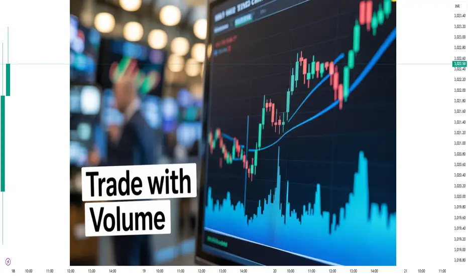
Basics of Volume AnalysisIntroduction
Volume is one of the most crucial yet underrated elements in trading and technical analysis. While most traders focus on price alone, professionals know that volume provides the fuel behind price movements. It answers the “how much” behind the “how far.” In simple words, volume tells us the strength or weakness of a move.
Without volume, price movement can be misleading because a rally or sell-off without sufficient participation may not sustain. Hence, understanding and analyzing volume correctly can help traders distinguish between real moves and false signals.
This comprehensive guide explains the basics of volume analysis, its role in trading, the theories behind it, and how traders can practically use it to improve decision-making.
Chapter 1: What is Volume in Trading?
Volume refers to the total number of shares, contracts, or lots traded in a particular asset within a specified time frame (such as 1 minute, 5 minutes, daily, or weekly).
For example:
If 10,000 shares of Reliance Industries are traded in one day, then the daily volume of Reliance is 10,000 shares.
In futures and options, volume refers to the number of contracts bought and sold.
In forex trading, volume is usually represented as the number of ticks (price changes) in a given time.
Key Points About Volume:
Volume measures activity and participation in the market.
High volume means greater interest and liquidity.
Low volume means lack of participation and higher risk of false moves.
Volume is relative — 100,000 shares traded in a small-cap stock may be considered high, but the same volume in a large-cap stock may be low.
Chapter 2: Importance of Volume in Trading
Why should traders pay attention to volume? Because price without volume is like a car without fuel.
1. Confirmation of Trend
Rising prices with rising volume = strong uptrend.
Falling prices with rising volume = strong downtrend.
Rising prices with falling volume = weak uptrend (may reverse).
Falling prices with falling volume = weak downtrend (may reverse).
2. Identifying Reversals
Volume often spikes at major reversal points, as large traders and institutions enter or exit.
3. Recognizing Breakouts and Breakdowns
Breakout above resistance with strong volume = reliable.
Breakout above resistance with weak volume = false breakout risk.
4. Detecting Accumulation and Distribution
High volume near support levels suggests accumulation by smart money.
High volume near resistance suggests distribution (selling).
5. Liquidity & Execution
High-volume assets are easier to trade with minimal slippage.
Chapter 3: Theories Behind Volume Analysis
Several technical analysis theories stress the role of volume:
1. Dow Theory and Volume
Charles Dow, father of modern technical analysis, said volume must confirm the trend.
In an uptrend, volume should increase as prices rise and decrease on pullbacks.
In a downtrend, volume should increase as prices fall and decrease on rallies.
2. Volume Precedes Price
Many times, volume surges before price makes a significant move. Institutions build positions quietly, and this hidden activity shows up in volume before the price breakout.
3. Effort vs. Result Principle (Wyckoff Theory)
Effort = volume
Result = price movement
If effort (volume) is high but result (price move) is small, it indicates hidden resistance or absorption.
Chapter 4: Types of Volume Analysis
1. Simple Volume Analysis
Looking at volume bars below a candlestick chart to see if it confirms price movement.
2. Relative Volume
Comparing today’s volume with average historical volume.
Example: If a stock’s average daily volume is 1 million shares, but today it trades 5 million, something important is happening.
3. Volume Oscillators and Indicators
Many indicators are built on volume, such as:
On-Balance Volume (OBV)
Volume Weighted Average Price (VWAP)
Accumulation/Distribution Line
Chaikin Money Flow
Volume Price Trend (VPT)
Chapter 5: Practical Techniques of Volume Analysis
1. Volume with Support and Resistance
A breakout above resistance with high volume = trend continuation.
A breakout with low volume = false signal.
2. Volume Spikes
Sudden large increases in volume usually precede strong price moves or mark exhaustion at tops/bottoms.
3. Volume Divergence
If price makes new highs but volume decreases, the trend is weakening.
4. Volume in Consolidation
Low volume during sideways movement = healthy consolidation.
Rising volume in sideways = accumulation or distribution.
5. Volume & Candlestick Patterns
Bullish engulfing with high volume = strong reversal.
Doji with high volume = uncertainty and potential turning point.
Chapter 6: Popular Volume Indicators
1. On-Balance Volume (OBV)
OBV adds volume on up days and subtracts on down days. It helps identify accumulation or distribution trends.
2. Volume Weighted Average Price (VWAP)
VWAP shows the average price at which a stock has traded throughout the day, weighted by volume. Used by institutions for fair value.
3. Accumulation/Distribution Line
Measures how much of a stock’s volume is flowing in or out.
4. Chaikin Money Flow (CMF)
Shows buying and selling pressure over a period based on volume and closing price.
5. Volume Price Trend (VPT)
Combines percentage price change with volume to confirm strength of trends.
Chapter 7: Volume in Different Timeframes
1. Intraday Trading
Intraday traders use volume spikes to enter momentum trades.
VWAP is critical for institutional intraday positions.
2. Swing Trading
Swing traders watch volume on breakout of ranges.
They avoid low-volume stocks as moves may not sustain.
3. Long-Term Investing
Investors analyze accumulation phases with high volume at bottoms.
Volume helps identify institutional entry points.
Chapter 8: Case Studies
Example 1: Breakout Confirmation
Suppose Infosys stock has been consolidating between ₹1,400–₹1,450 for months. One day, it breaks above ₹1,450 with 3x average volume. This confirms buyers’ strength, and price is likely to sustain upward.
Example 2: False Breakout
Another stock breaks above resistance but on very low volume. Price quickly falls back. Here, volume warned traders of a trap.
Example 3: Market Tops
At market peaks, price may still rise, but volume gradually declines. This divergence signals weakening demand.
Chapter 9: Limitations of Volume Analysis
Different Markets Measure Volume Differently: Forex uses tick volume, not actual trade volume.
False Signals: High volume can also occur due to news or rumors, leading to traps.
Not Standalone: Should be combined with price action, trend analysis, and indicators.
Institutional Tricks: Smart money sometimes creates artificial volume to mislead retail traders.
Chapter 10: Best Practices for Traders
Always compare volume with price action, not alone.
Use relative volume (compare with historical averages).
Combine with technical tools like candlestick patterns, moving averages, or VWAP.
Avoid illiquid stocks with low volume.
Watch for volume divergences — they often precede reversals.
For intraday, focus on the first 30 minutes and last 30 minutes when volume is highest.
Conclusion
Volume analysis is like the heartbeat of the market. It reveals the hidden intentions of big players, confirms the strength of moves, and warns against false signals. By mastering volume, traders can improve their accuracy in identifying trends, reversals, breakouts, and consolidations.
While volume is not perfect and should not be used in isolation, it is one of the most powerful tools when combined with price action and other indicators. From Dow Theory to modern-day VWAP strategies, volume continues to be a central pillar of trading success.
For beginners, the journey starts with simply observing volume bars on price charts and gradually moving to advanced concepts like OBV, VWAP, and Wyckoff’s effort vs. result principle. Over time, volume analysis becomes second nature, helping traders see beyond the surface of price and into the market’s underlying strength.
X-indicator
Quarterly Results Trading in BanksIntroduction
Banking stocks hold a special place in the financial markets. Whether in India, the U.S., or any other part of the world, banks act as the backbone of the economy. Their quarterly earnings are closely tracked by investors, traders, regulators, and even policymakers because banks represent the health of credit growth, liquidity, interest rate transmission, and corporate activity.
Quarterly results trading in banks is a niche yet powerful strategy where traders position themselves before, during, or after the announcement of bank earnings. The volatility surrounding these results often creates opportunities for both short-term and swing traders. However, this is not a simple “buy on results day” strategy—success depends on understanding earnings drivers, market expectations, macroeconomic context, and technical setups.
This guide explores quarterly results trading in banks in-depth—covering how to analyze reports, predict moves, trade around volatility, and manage risks.
1. Why Bank Quarterly Results Matter
Banks are interest-rate-sensitive and macro-sensitive businesses. Their results reflect not just their own performance but also the broader economy. Let’s break down why they matter:
1.1 Indicators of Economic Health
Banks’ loan growth signals demand from businesses and consumers.
Non-Performing Assets (NPAs) show stress in corporate and retail borrowers.
Net Interest Margins (NIMs) indicate efficiency in lending vs borrowing costs.
1.2 Policy and Liquidity Sensitivity
RBI (or Fed in the U.S.) interest rate decisions directly impact banks’ earnings.
Liquidity conditions affect treasury gains/losses.
1.3 Heavyweights in Indices
In India, banks form a large chunk of Nifty 50 and Bank Nifty. Thus, quarterly results of major banks (HDFC Bank, ICICI Bank, SBI, Axis Bank, Kotak Bank) can swing the entire index.
1.4 Investor and FII Interest
Foreign Institutional Investors (FIIs) actively trade banking stocks, making them liquid and volatile during results season.
2. Anatomy of a Bank’s Quarterly Results
Unlike manufacturing or IT companies, banks have unique reporting metrics. Traders must understand these before making moves.
2.1 Key Metrics to Track
Net Interest Income (NII): Interest earned from loans minus interest paid on deposits.
Net Interest Margin (NIM): Profitability of lending.
Loan Growth: Total advances YoY and QoQ.
Deposit Growth: CASA (Current Account Savings Account) ratio is crucial.
Non-Performing Assets (NPA): Gross NPA and Net NPA indicate asset quality.
Provision Coverage Ratio (PCR): Measures buffer against bad loans.
Fee Income & Treasury Gains: Non-interest revenue streams.
Return on Assets (ROA) & Return on Equity (ROE): Profitability indicators.
2.2 Segment-Wise Performance
Retail vs Corporate lending.
Infrastructure/SME lending trends.
Digital banking adoption.
2.3 Market Expectations
Results are judged not in isolation but against analyst expectations and guidance. Example:
If HDFC Bank posts 20% profit growth but analysts expected 25%, the stock may fall.
A small improvement in NPAs can trigger a rally even if profits are flat.
3. Market Psychology Around Quarterly Results
Quarterly results trading is less about numbers and more about expectations vs reality.
3.1 Pre-Result Rally (Speculation Phase)
Traders anticipate strong/weak results and position themselves early.
Stocks often run up 5–10% before results, only to correct after the announcement (“buy the rumor, sell the news”).
3.2 Result Day Volatility
Options premiums shoot up due to high implied volatility (IV).
Directional moves are sharp but unpredictable.
3.3 Post-Result Trends
The first reaction may be wrong; big players (FIIs, mutual funds) enter gradually, leading to multi-day trends.
Example: A bank stock might dip on profit miss but later rally when analysts highlight improved asset quality.
4. Trading Strategies Around Quarterly Results
Now comes the actionable part—how traders actually make money from quarterly results.
4.1 Pre-Result Trading
4.1.1 Momentum Play
Look for stocks showing strong buildup in price and volume before results.
Example: If ICICI Bank is rising steadily with delivery-based buying, traders may ride the momentum expecting strong numbers.
4.1.2 Options Straddle/Strangle
Since results bring volatility, traders use long straddles/strangles (buying both call and put options) to benefit from big moves.
Works best if IV is not too high.
4.1.3 Sectoral Sympathy Play
If HDFC Bank posts strong results, peers like Axis and Kotak may also rally even before their results.
4.2 Result Day Trading
4.2.1 Intraday Reaction Trading
Trade the immediate move after numbers are announced.
Example: Profit beats + lower NPAs = bullish candle = intraday long.
4.2.2 Fade the Overreaction
Sometimes the market overreacts.
Example: Stock falls 4% on slightly weak profit but asset quality improved—smart traders buy the dip.
4.2.3 Options IV Crush Strategy
Results announcement causes implied volatility to collapse.
Traders can sell straddles/strangles just before results to capture premium decay.
4.3 Post-Result Trading
4.3.1 Trend Following
Strong results often lead to multi-week rallies.
Example: SBI after strong quarterly results in 2023 kept rising for weeks.
4.3.2 Analyst Upgrade/Downgrade Reaction
Monitor brokerage reports. Stocks move sharply when Goldman, CLSA, or Nomura revise targets.
4.3.3 Pair Trading
Go long on strong-result bank and short on weak-result peer.
Example: Long ICICI Bank (good results), short Kotak Bank (disappointing results).
5. Case Studies: Quarterly Results Trading in Indian Banks
5.1 HDFC Bank Q1 FY24
Profit grew 30%, NII rose strongly.
Stock initially fell due to merger concerns but rallied later as analysts upgraded.
Lesson: First-day reaction is not always final.
5.2 SBI Q3 FY23
Record profits + lowest NPAs in decades.
Stock rallied 8% in 2 days.
Lesson: Asset quality improvement drives big moves.
5.3 ICICI Bank Q2 FY23
Strong NIMs, digital growth.
Stock jumped 10% in a week, leading Bank Nifty higher.
Lesson: Market rewards consistency.
6. Risk Management in Quarterly Results Trading
6.1 Position Sizing
Never go all-in on result day. Limit exposure to 2–5% of portfolio.
6.2 Volatility Protection
Use options to hedge positions. For example, buy puts if holding large long positions.
6.3 Avoid Overtrading
Many traders burn capital chasing every tick. Results volatility is sharp; patience pays.
6.4 Macro Factors
Even if bank results are strong, global factors (Fed hikes, crude oil, FII outflows) may drag stocks down.
7. Tools and Analysis Methods
7.1 Technical Analysis
Support/Resistance Levels for pre-result positioning.
Volume Profile to track accumulation/distribution.
Candlestick Patterns post-results for confirmation.
7.2 Fundamental Analysis
Compare QoQ and YoY trends.
Peer comparison to judge relative performance.
7.3 Sentiment Analysis
Track news, social media, and analyst expectations.
7.4 Options Data
Open Interest (OI) buildup signals trader positioning.
PCR (Put-Call Ratio) indicates sentiment.
8. Opportunities & Pitfalls
8.1 Opportunities
Volatility-driven profits.
Strong trending moves after results.
Options strategies like IV crush trading.
8.2 Pitfalls
Overestimating results impact.
Ignoring macro/global triggers.
Getting trapped in whipsaws.
Holding naked option positions.
9. Quarterly Results Trading vs Other Earnings Plays
Banks: Highly macro-driven, sensitive to RBI/Fed.
IT Sector: More dependent on U.S. client spending and forex.
FMCG: Stable, less volatile.
Thus, bank results trading = high risk, high reward.
10. Long-Term Implications of Quarterly Results
While traders focus on short-term gains, quarterly results also help investors:
Identify consistent compounders like HDFC Bank or ICICI Bank.
Spot early signs of stress (like Yes Bank before its collapse).
Gauge sectoral shifts—retail vs corporate lending trends.
Conclusion
Quarterly results trading in banks is not just about reacting to numbers—it’s about interpreting expectations, economic signals, market psychology, and technical setups. The volatility around earnings gives traders multiple opportunities: pre-result speculation, result-day intraday plays, and post-result trend following.
But it is also one of the riskiest forms of trading because moves can be unpredictable. Success depends on discipline, risk management, and a balanced approach combining fundamentals with technicals.
In India, where banking stocks dominate indices like Nifty and Bank Nifty, mastering quarterly results trading can give traders a serious edge. The key is not just to chase profits but to understand the story behind the numbers.
Part 2 Candle Sticks PatternHow Options Work in Trading
Imagine a stock is trading at ₹1,000.
You believe it will rise to ₹1,100 in a month. You could:
Buy the stock: You need ₹1,000 per share.
Buy a call option: You pay a small premium (say ₹50) for the right to buy at ₹1,000 later.
If the stock rises to ₹1,100:
Stock profit = ₹100
Call option profit = ₹100 (intrinsic value) - ₹50 (premium) = ₹50 net profit (but with much lower capital).
This leverage makes options attractive but also risky — if the stock doesn’t rise, your premium is lost.
Categories of Options Strategies
Options strategies can be divided into three main categories:
Directional Strategies – Profit from price movements.
Non-Directional (Neutral) Strategies – Profit from sideways markets.
Hedging Strategies – Protect existing positions.
Directional Strategies
These are for traders with a clear market view.

Learn Institutional TradingIntroduction to Options Trading
Options trading is one of the most flexible and powerful tools in the financial markets. Unlike stocks, where you simply buy and sell ownership of a company, options are derivative contracts that give you the right, but not the obligation, to buy or sell an underlying asset at a predetermined price within a specified time frame.
The beauty of options lies in their strategic possibilities — they allow traders to make money in rising, falling, or even sideways markets, often with less capital than buying stocks outright. But with that flexibility comes complexity, so understanding strategies is crucial.
Key Terms in Options Trading
Before we jump into strategies, let’s understand the key terms:
Call Option – Gives the right to buy the underlying asset at a fixed price (strike price) before expiry.
Put Option – Gives the right to sell the underlying asset at a fixed price before expiry.
Strike Price – The price at which you can buy/sell the asset.
Premium – The price you pay to buy an option.
Expiry Date – The date the option contract ends.
ITM (In-the-Money) – When exercising the option would be profitable.
ATM (At-the-Money) – Strike price is close to the current market price.
OTM (Out-of-the-Money) – Option has no intrinsic value yet.
Lot Size – Minimum number of shares/contracts per option.
Intrinsic Value – The real value if exercised now.
Time Value – Extra premium based on time left to expiry.

Part 4 Learn Institutional TradingProtective Put
When to Use: To insure against downside.
Setup: Own stock + Buy put option.
Risk: Premium paid.
Reward: Stock can rise, but downside is protected.
Example: Own TCS at ₹3,000, buy 2,900 PE for ₹50.
Bull Call Spread
When to Use: Expect moderate rise.
Setup: Buy lower strike call + Sell higher strike call.
Risk: Limited.
Reward: Limited.
Example: Buy 20,000 CE @ ₹100, Sell 20,200 CE @ ₹50.
Bear Put Spread
When to Use: Expect moderate fall.
Setup: Buy higher strike put + Sell lower strike put.
Risk: Limited.
Reward: Limited.

Part 3 Learn Institutional TradingDirectional Strategies
These are for traders with a clear market view.
Long Call (Bullish)
When to Use: Expecting significant upward movement.
Setup: Buy a call option.
Risk: Limited to premium paid.
Reward: Unlimited.
Example: NIFTY at 20,000, you buy 20,100 CE for ₹100 premium. If NIFTY closes at 20,500, your profit = ₹400 - ₹100 = ₹300.
Long Put (Bearish)
When to Use: Expecting price drop.
Setup: Buy a put option.
Risk: Limited to premium.
Reward: Large if the asset falls.
Example: Stock at ₹500, buy 480 PE for ₹10. If stock drops to ₹450, profit = ₹30 - ₹10 = ₹20.
Covered Call (Mildly Bullish)
When to Use: Own the stock but expect limited upside.
Setup: Hold stock + Sell call option.
Risk: Stock downside risk.
Reward: Premium income + stock gains until strike price.
Example: Own Reliance at ₹2,500, sell 2,600 CE for ₹20 premium.

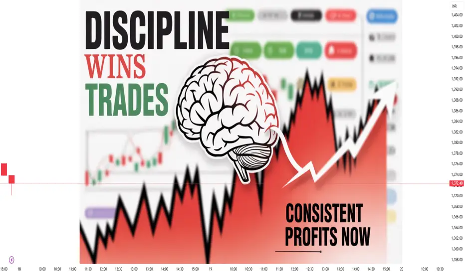
Trading Discipline with Biofeedback1. Introduction: Why Trading Discipline is Hard
In the world of financial markets, traders are constantly balancing analysis with emotion. Charts and data may look purely rational, but the human brain does not operate like a spreadsheet. Instead, traders face fear, greed, overconfidence, hesitation, and impulse — all in rapid cycles during market hours.
Trading discipline is the ability to execute a trading plan consistently, without being swayed by emotional impulses or external noise. It’s what separates a professional who survives years in the market from someone who burns out after a few months.
The challenge? Even the best-prepared trader can watch their discipline crumble in moments of market stress. This is where biofeedback comes in — a method for measuring and controlling physiological responses to improve self-control and decision-making under pressure.
2. What is Biofeedback in the Context of Trading?
Biofeedback is a technique where you use electronic monitoring devices to measure physiological functions — like heart rate, breathing rate, muscle tension, skin conductance, and brainwave activity — and then use that real-time data to learn how to control them.
In trading, biofeedback can help you:
Recognize early signs of stress before they impact your judgment.
Maintain an optimal arousal level for peak performance.
Train your nervous system to remain calm in volatile situations.
Develop habits that strengthen mental resilience over time.
Example:
A trader using a heart rate variability (HRV) monitor might notice their HRV drops significantly before a losing trade — a sign of rising stress. With practice, they can use breathing techniques to restore calm and prevent impulsive decisions.
3. The Science Behind Biofeedback for Traders
3.1. The Stress-Performance Curve
This is based on the Yerkes–Dodson Law, which shows that performance improves with physiological arousal — but only up to a point. Too little arousal (low alertness) leads to sluggish reactions; too much (high anxiety) causes poor judgment.
Biofeedback helps traders stay in the optimal performance zone — alert but calm.
3.2. Physiological Markers in Trading
When you place a trade or watch a volatile market, your body activates the sympathetic nervous system ("fight-or-flight" mode):
Heart rate increases → decision-making becomes reactive.
Breathing shortens → oxygen supply to the brain decreases.
Skin conductance rises → higher sweat response from stress.
Muscle tension increases → physical discomfort, fatigue.
Brainwaves shift → from alpha/theta (calm focus) to high beta (stress).
This physiological shift can override logic. Biofeedback helps you detect these changes before they hijack your behavior.
3.3. Neuroplasticity and Habit Formation
Biofeedback training taps into neuroplasticity — the brain’s ability to rewire itself through repeated experience. By pairing specific mental states (calm focus) with trading activities, you strengthen neural pathways that make discipline more automatic.
4. Why Discipline Breaks in Trading
Even with a perfect trading plan, discipline often fails because:
Emotional Hijacking — The amygdala overrides rational thought under stress.
Overtrading — Dopamine-driven urge to "chase" trades after wins or losses.
Loss Aversion — The tendency to avoid losses at all costs, leading to holding losers too long.
Confirmation Bias — Seeking only information that supports your existing trade.
Fatigue — Poor sleep or extended screen time reduces impulse control.
Biofeedback directly addresses points 1 and 5, and indirectly helps with the rest by improving awareness and emotional regulation.
5. Types of Biofeedback Tools for Traders
5.1. Heart Rate Variability (HRV) Monitors
Function: Measures beat-to-beat variations in heart rate.
Why it’s useful: Higher HRV = greater resilience and adaptability to stress.
Popular devices: Polar H10, Whoop, Elite HRV, Oura Ring.
5.2. Electroencephalography (EEG) Headsets
Function: Measures brainwave activity (alpha, beta, theta, gamma).
Why it’s useful: Identifies mental states — e.g., focus, relaxation, distraction.
Popular devices: Muse, Emotiv Insight.
5.3. Skin Conductance Sensors
Function: Measures electrical conductance of skin (linked to sweat response).
Why it’s useful: Early indicator of stress before conscious awareness.
Popular devices: Empatica E4, GSR2.
5.4. Breathing Feedback Devices
Function: Tracks breathing rate and depth.
Why it’s useful: Calm, diaphragmatic breathing maintains optimal arousal levels.
Popular devices: Spire Stone, Breathbelt.
5.5. Multi-Sensor Platforms
Combine HRV, skin conductance, temperature, movement, and EEG for a full picture.
Often integrated with mobile apps that guide breathing, meditation, or cognitive training.
6. The Biofeedback-Discipline Loop for Traders
Here’s how biofeedback fits into a trader’s workflow:
Baseline Measurement
Monitor your physiological state during calm, non-trading hours.
Establish "normal" HRV, heart rate, and brainwave patterns.
Stress Mapping
Record your physiological data during live trading.
Identify patterns before, during, and after trades — especially losing streaks.
Intervention Training
Use breathing, mindfulness, or focus exercises to restore optimal state.
Repeat until the intervention becomes automatic.
Real-Time Application
Wear biofeedback devices during trading.
Take action the moment stress markers exceed thresholds.
Review and Adjust
Analyze post-trade logs for emotional triggers and physiological patterns.
Update your discipline strategy accordingly.
7. Biofeedback Training Protocol for Traders
Phase 1: Awareness (2–3 Weeks)
Goal: Understand your physiological reactions to market events.
Action Steps:
Wear HRV and skin conductance sensors during trading.
Log market conditions and emotional states alongside data.
Identify recurring "stress spikes" and the situations causing them.
Phase 2: Regulation (3–4 Weeks)
Goal: Learn to control physiological stress responses.
Techniques:
Coherent Breathing: Inhale for 5.5 seconds, exhale for 5.5 seconds.
Progressive Muscle Relaxation: Tense and release muscles from head to toe.
Alpha Wave Training: Use EEG feedback to enter calm, focused states.
Phase 3: Integration (Ongoing)
Goal: Make emotional regulation part of your trading routine.
Action Steps:
Pre-market: 5 minutes of HRV breathing.
During trading: Monitor stress markers, take breaks if needed.
Post-market: Review biofeedback logs and trade journal together.
8. Case Studies
Case Study 1: The Impulsive Scalper
Problem: A day trader entered trades too quickly after losses, leading to overtrading.
Biofeedback Insight: HRV dropped sharply after losing trades; breathing became shallow.
Solution: Implemented 3-minute breathing reset after each loss. Over 6 weeks, reduced revenge trades by 70%.
Case Study 2: The Swing Trader with Exit Anxiety
Problem: Took profits too early due to fear of reversals.
Biofeedback Insight: EEG showed increased beta waves when price approached target.
Solution: Practiced alpha-wave breathing before exit decisions. Result: Average holding time increased by 15%, boosting profits.
Case Study 3: The New Trader with Market Open Stress
Problem: Felt overwhelmed at the opening bell, making erratic trades.
Biofeedback Insight: Skin conductance spiked dramatically at market open.
Solution: Added 10 minutes of pre-market meditation and HRV training. Result: 40% fewer impulsive trades in the first 30 minutes.
9. Advantages of Biofeedback for Trading Discipline
Objective self-awareness: Replaces guesswork with measurable data.
Prevents emotional spirals: Stops small mistakes from snowballing.
Speeds up learning: Accelerates habit formation for calm decision-making.
Customizable: Can be adapted to each trader’s unique stress patterns.
Integrates with trading journal: Creates a full picture of both mental and market performance.
10. Limitations and Considerations
Cost: High-quality devices can be expensive.
Learning curve: Requires time to interpret data and apply techniques.
Over-reliance: Biofeedback should enhance, not replace, psychological skill-building.
Privacy: Data storage should be secure, especially with cloud-based apps.
Conclusion
Trading discipline is not just a mental skill — it’s a mind-body skill. Biofeedback bridges the gap between the psychological and physiological sides of trading performance. By learning to recognize and control your body’s stress responses, you can keep your decision-making sharp, your execution consistent, and your emotions balanced even in high-pressure market environments.
Over time, biofeedback training rewires your nervous system for resilience, turning discipline from a constant battle into a natural, automatic state. And in the competitive world of trading, that could be the difference between long-term success and early burnout.
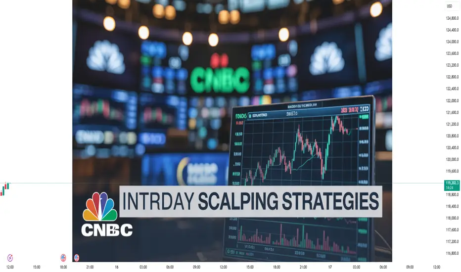
Intraday Scalping & Momentum Trading1. Introduction
In the high-speed world of financial markets, two strategies stand out for traders who thrive on quick decisions and rapid results: Intraday Scalping and Momentum Trading.
While both are short-term trading styles, they differ in execution speed, trade duration, and the logic behind entries and exits.
Intraday Scalping focuses on capturing tiny price movements — sometimes just a few points — multiple times throughout the trading session.
Momentum Trading aims to ride significant price moves caused by strong buying or selling pressure, often holding positions for minutes to hours until the trend exhausts.
In both strategies:
Speed is critical.
Precision is non-negotiable.
Discipline is the backbone.
2. The Core Concepts
2.1 Intraday Scalping
Scalping is like market sniping — taking small, precise shots. The goal is not to hit a home run but to consistently hit singles that add up.
Key traits:
Very short holding times (seconds to a few minutes).
Multiple trades per day (5–50+ depending on style).
Targets are small (0.1%–0.5% price move per trade).
Relies on high liquidity and tight bid-ask spreads.
Example:
Stock XYZ is trading at ₹100.25/₹100.30.
Scalper buys at ₹100.30.
Price ticks up to ₹100.40 in 30 seconds.
Exit at ₹100.40 — profit of ₹0.10 per share.
Tools used:
Level 2 order book (market depth).
Time & sales tape.
Tick charts (1-min, 15-sec).
Volume profile for micro-trends.
2.2 Momentum Trading
Momentum trading is like surfing a wave. Once a strong move starts (due to news, earnings, sector activity, or breakout), momentum traders jump in to ride the surge until it slows.
Key traits:
Holding time is longer than scalping (minutes to hours).
Focus on directional moves with high relative volume.
Larger price targets (0.5%–3% or more per trade).
Relies on trend continuation until exhaustion.
Example:
Stock ABC breaks resistance at ₹250 on high volume after earnings.
Trader buys at ₹252 expecting further upside.
Price runs to ₹260 before showing weakness.
Exit at ₹259 — profit of ₹7 per share.
Tools used:
1-min to 15-min charts.
Moving averages for trend confirmation.
Relative Volume (RVOL) scanners.
Momentum oscillators like RSI, MACD.
3. Scalping vs Momentum — Quick Comparison
Feature Scalping Momentum Trading
Trade Duration Seconds to few minutes Minutes to hours
Profit Target 0.1%–0.5% 0.5%–3%+
Risk per Trade Very small Small to medium
Frequency High (10–50 trades/day) Moderate (2–10 trades/day)
Chart Timeframes Tick, 15s, 1m 1m, 5m, 15m
Market Conditions High liquidity, volatile Trending, news-driven
Mindset Ultra-fast decisions Patient within trend
4. Market Conditions Suitable for Each
Scalping Works Best When:
Market is choppy but liquid.
Bid-ask spread is tight.
Price moves in micro-waves.
There is high intraday volatility without a clear trend.
Momentum Works Best When:
Market has strong trend days.
There’s a news catalyst or earnings.
Breakouts/breakdowns occur with volume surge.
A sector rotation drives capital into specific stocks.
5. Technical Tools & Indicators
For Scalping
VWAP (Volume Weighted Average Price) – Used as a magnet for price action; scalpers fade moves away from VWAP or trade rejections.
EMA 9 & EMA 20 – For micro-trend direction.
Order Flow Analysis – Reading the tape to identify big orders.
Bollinger Bands (1-min) – Spotting overextensions.
Volume Profile – Identifying intraday support/resistance.
For Momentum
Moving Averages (EMA 20, EMA 50) – Identify trend continuation.
MACD – Confirm momentum strength.
RSI (5 or 14 period) – Spotting overbought/oversold within a trend.
Breakout Levels – Pre-marked resistance/support zones.
Relative Volume (RVOL) – Ensures trade is supported by unusual buying/selling pressure.
6. Strategies
6.1 Scalping Strategies
A) VWAP Bounce Scalping
Wait for price to pull back to VWAP after a quick move.
Enter on rejection candles.
Exit after a small bounce.
B) Breakout Scalping
Identify micro-breakouts from 1-min consolidation.
Enter just before the breakout.
Exit within seconds once target is hit.
C) Market Maker Following
Watch for large limit orders on Level 2.
Follow their buying/selling pressure.
Exit when big order disappears.
6.2 Momentum Strategies
A) News Catalyst Plays
Scan for stocks with fresh positive/negative news.
Wait for first pullback after breakout.
Ride until momentum slows.
B) Trend Continuation
Identify stock above VWAP and moving averages.
Enter on EMA 9/EMA 20 bounce.
Exit when price closes below EMA 20.
C) High Relative Volume Breakouts
Use RVOL > 2.0 filter.
Enter when volume spikes confirm breakout.
Place stop-loss just under breakout level.
7. Risk Management
Both scalping and momentum trading require tight stop-losses because small moves against you can quickly turn into bigger losses.
For Scalping:
Stop-loss: 0.1%–0.3%.
Risk per trade: ≤ 0.5% of account.
Don’t average down — cut losses immediately.
For Momentum:
Stop-loss: 0.5%–1.5%.
Risk per trade: ≤ 1% of account.
Trail stops to lock in profits.
General Rules:
Use position sizing: Risk Amount ÷ Stop Size = Position Size.
Always account for slippage.
Never risk more than you can afford to lose in a single day.
8. Trading Psychology
For Scalpers:
Stay hyper-focused. Avoid hesitation. The moment you second-guess, the trade is gone. Mental fatigue sets in quickly — take breaks.
For Momentum Traders:
Patience is key. Don’t exit too early from fear or greed. Stick to the plan and avoid chasing after missed moves.
Mind Traps to Avoid:
Overtrading.
Revenge trading after a loss.
Ignoring stop-loss because “it might bounce back.”
Letting small losses turn into big ones.
9. Examples of a Trading Day
Scalping Example
9:20 AM: Identify stock XYZ near pre-market resistance.
9:25 AM: Scalper enters on small pullback.
9:26 AM: Price moves 0.15% up — exit instantly.
Repeat 12–15 times, ending with 8 wins, 4 losses.
Momentum Example
9:25 AM: News drops on ABC Ltd.
9:30 AM: Stock gaps up 3%, breaks resistance with volume.
Buy at ₹252, hold for 20 minutes as it climbs to ₹259.
Exit when volume declines and price closes under EMA 20.
10. Common Mistakes
Scalping:
Entering in low-volume stocks → big slippage.
Over-leveraging.
Trading during low volatility periods.
Momentum:
Chasing moves without pullback.
Ignoring broader market trend.
Overstaying in trade after momentum fades.
11. Advanced Tips
Use hotkeys to speed up entries and exits.
Trade during high liquidity hours (first and last 90 minutes of market).
Combine pre-market analysis with real-time setups.
Keep a trading journal to refine entries/exits.
12. Conclusion
Intraday Scalping and Momentum Trading are high-performance trading styles that can generate consistent profits for skilled traders — but they’re not for the faint-hearted.
They require:
Quick decision-making.
Iron discipline.
Solid risk management.
Technical precision.
The golden rule is: protect your capital first, profits will follow.
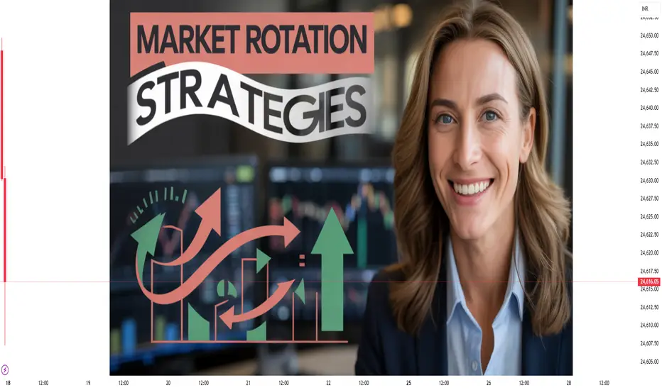
Market Rotation Strategies1. Introduction to Market Rotation
Market rotation (also called sector rotation or capital rotation) is a strategy where traders and investors shift their capital between different asset classes, sectors, or investment styles based on economic conditions, market sentiment, and performance trends.
The idea is simple: money flows like a river — it doesn’t disappear, it just changes direction. By positioning yourself where the money is flowing, you can potentially capture higher returns and reduce drawdowns.
Example: In an economic boom, technology and consumer discretionary stocks may outperform. But during a slowdown, utilities and healthcare might take the lead.
2. Why Market Rotation Works
Market rotation works because of capital flow dynamics. Institutional investors, hedge funds, pension funds, and large asset managers reallocate capital based on:
Economic Cycle – Growth, peak, contraction, and recovery phases affect which sectors lead or lag.
Interest Rates – Rising or falling rates change the attractiveness of certain assets.
Earnings Growth Expectations – Sectors with better forward earnings tend to attract inflows.
Risk Appetite – “Risk-on” phases favor aggressive sectors; “risk-off” phases favor defensive sectors.
Rotation strategies aim to front-run or follow these capital shifts.
3. Types of Market Rotation
Market rotation isn’t just about sectors. It happens across various dimensions:
A. Sector Rotation
Shifting between market sectors (e.g., tech, energy, financials, healthcare) depending on performance and macroeconomic signals.
Example Pattern in a Typical Economic Cycle:
Early Expansion: Industrials, Materials, Financials
Mid Expansion: Technology, Consumer Discretionary
Late Expansion: Energy, Basic Materials
Recession: Utilities, Healthcare, Consumer Staples
B. Style Rotation
Shifting between different investing styles such as:
Growth vs. Value
Large-cap vs. Small-cap
Dividend vs. Non-dividend stocks
Example: When interest rates rise, value stocks often outperform growth stocks.
C. Asset Class Rotation
Shifting between stocks, bonds, commodities, real estate, or even cash based on macroeconomic conditions.
Example: Moving from equities to bonds before an expected recession.
D. Geographic Rotation
Allocating funds between different countries or regions.
Example: Rotating from U.S. equities to emerging markets when global growth broadens.
4. The Economic Cycle & Market Rotation
Understanding the economic cycle is critical for timing rotations.
Four Main Phases:
Early Recovery: GDP starts growing, interest rates are low, credit expands.
Mid Cycle: Growth strong, inflation starts rising, central banks begin tightening.
Late Cycle: Growth slows, inflation high, corporate profits peak.
Recession: GDP contracts, unemployment rises, central banks cut rates.
Sector Leaders by Cycle:
Economic Phase Leading Sectors
Early Recovery Industrials, Financials, Technology
Mid Cycle Consumer Discretionary, Industrials, Tech
Late Cycle Energy, Materials, Healthcare
Recession Utilities, Consumer Staples, Healthcare
5. Tools & Indicators for Rotation Strategies
A. Relative Strength (RS) Analysis
Compares the performance of a sector/asset to a benchmark (e.g., S&P 500).
RS > 1: Outperforming
RS < 1: Underperforming
B. Moving Averages
Track momentum trends in sector ETFs or indexes.
50-day & 200-day MA crossovers can signal when to rotate.
C. MACD & RSI
Momentum oscillators can indicate when a sector is overbought/oversold.
D. Intermarket Analysis
Study correlations between:
Stocks & Bonds
Commodities & Currencies
Oil prices & Energy stocks
E. Economic Data
Key data points for rotation:
PMI (Purchasing Managers Index)
Inflation (CPI, PPI)
Interest Rate Trends
Earnings Reports
6. Step-by-Step: Building a Market Rotation Strategy
Step 1 – Define Your Universe
Choose what you’ll rotate between:
S&P 500 sectors (using ETFs like XLK for tech, XLF for financials)
Style indexes (e.g., Growth vs Value ETFs)
Asset classes (SPY, TLT, GLD, etc.)
Step 2 – Choose Your Indicators
Example:
3-month relative performance vs S&P 500
Above 50-day MA = bullish
Below 50-day MA = bearish
Step 3 – Establish Rotation Rules
Example:
Every month, buy the top 3 sectors ranked by RS.
Hold until the next review period.
Exit if RS drops below 0.9 or price closes below 200-day MA.
Step 4 – Risk Management
Max 20-30% of portfolio per sector
Stop-loss of 8-10% per position
Cash position allowed when no sector meets criteria
Step 5 – Backtest
Use historical data for at least 10 years.
Compare performance vs buy-and-hold S&P 500.
7. Example Rotation Strategy
Universe: 9 SPDR Sector ETFs
Indicator: 3-month price performance
Rules:
Each month, rank all sectors by 3-month returns.
Buy the top 3 equally weighted.
Hold for 1 month, then rebalance.
Exit if price drops below 200-day MA.
Result (historical):
Outperforms S&P 500 in trending markets.
Avoids big drawdowns in recessions.
8. Advanced Rotation Approaches
A. Factor Rotation
Rotate based on factors like:
Momentum
Low Volatility
Quality
Value
B. Tactical Asset Allocation (TAA)
Mix market rotation with risk-on/risk-off models.
Example:
Risk-on: Equities + Commodities
Risk-off: Bonds + Cash
C. Quantitative Rotation
Use algorithms to dynamically shift assets based on multi-factor models (momentum + macro + volatility).
D. Seasonal Rotation
Exploit seasonal trends.
Example: Energy stocks in winter, retail stocks in holiday season.
9. Risk Management in Market Rotation
Even with a rotation strategy:
Correlations can rise in market crashes (everything falls together).
Overtrading can eat into returns due to costs.
False signals can lead to whipsaws.
Mitigation:
Use confirmation from multiple indicators.
Diversify across at least 3 positions.
Keep cash buffer during high uncertainty.
10. Common Mistakes in Rotation Strategies
Chasing performance – Entering too late after a sector has already peaked.
Ignoring transaction costs – Frequent rebalancing reduces net gains.
Overfitting backtests – Strategy works historically but fails in real time.
Neglecting macro trends – Technicals alone may miss big shifts.
Conclusion
Market rotation strategies are about positioning capital where it has the highest probability of growth while avoiding weak areas.
Done right, rotation:
Improves returns
Reduces volatility
Aligns with economic and market cycles
But it requires discipline, data, and adaptability.
The market is dynamic — rotation strategies must evolve with it.
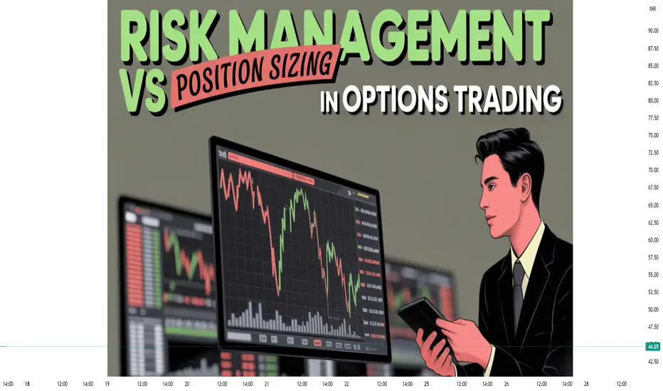
Risk Management & Position SizingRisk Management & Position Sizing: The Ultimate Trading Survival Blueprint
1. Introduction: Why Risk Management is the Real “Holy Grail” of Trading
If you spend time in trading communities or social media, you’ll often see traders obsessing over entry signals, technical indicators, and secret strategies. While these are important, they are not what keep a trader in the game over the long run.
The true difference between a consistent trader and a gambler lies in one thing:
Risk management.
You can have the best system in the world, but without risk control, one bad trade can wipe you out. On the other hand, even an average system can be profitable with proper risk and position sizing. This is why professional traders say:
“Your number one job is not to make money. It’s to protect your capital.”
“Risk what you can afford to lose, not what you hope to win.”
Risk management is not just about setting a stop-loss; it’s an entire framework for ensuring your account survives and grows steadily.
2. Understanding Risk in Trading
Before we talk about position sizing, we need to understand the different types of risk a trader faces:
2.1 Market Risk
The risk of losing money due to unfavorable price movements. This is the most obvious type and what stop-losses are designed to control.
2.2 Leverage Risk
Trading with borrowed capital can amplify both gains and losses. Over-leveraging is a common cause of account blow-ups.
2.3 Liquidity Risk
In illiquid markets, it might be hard to enter or exit at desired prices, leading to slippage.
2.4 Gap Risk
Overnight gaps or sudden news can cause prices to jump past your stop-loss, creating larger-than-expected losses.
2.5 Psychological Risk
Fear, greed, overconfidence, and revenge trading can lead to poor decisions.
3. The Two Pillars: Risk per Trade & Position Sizing
Risk management in trading has two main pillars:
Risk per trade – deciding how much of your account you’re willing to lose on a single trade.
Position sizing – calculating how many units, shares, or contracts you should trade based on your risk limit.
These two go hand in hand. You can’t size positions effectively unless you know your risk per trade.
4. Risk per Trade: The 1%–2% Rule
Most professional traders use a fixed percentage of their capital to determine risk per trade.
The most common guideline: risk 1–2% of your total trading capital per trade.
If your account is ₹5,00,000 and you risk 1% per trade, your maximum loss per trade = ₹5,000.
If you risk 2%, it’s ₹10,000.
Why this works:
It keeps losses small and survivable.
It allows you to take multiple trades without blowing up after a losing streak.
It aligns with long-term capital preservation.
Why Not Risk More?
Let’s say you risk 10% per trade and have a 5-trade losing streak:
Start: ₹5,00,000
After 1st loss (10%): ₹4,50,000
After 5th loss: ₹2,95,245 (down ~41%)
Recovering from that drawdown will require a massive +70% return.
5. Position Sizing: The Formula
Once you decide how much you’re willing to risk, you can calculate your position size.
Formula:
Position Size
=
Account Risk per Trade
Trade Risk per Unit
Position Size=
Trade Risk per Unit
Account Risk per Trade
Where:
Account Risk per Trade = Account Balance × % Risk per Trade
Trade Risk per Unit = Entry Price – Stop Loss Price
Example:
Account Balance: ₹5,00,000
Risk per trade: 1% = ₹5,000
Stock: Entry ₹250, Stop Loss ₹240 (risk ₹10 per share)
Position Size:
₹
5
,
000
₹
10
=
500
shares
₹10
₹5,000
=500 shares
You would buy 500 shares of that stock, risking ₹10 each for a total risk of ₹5,000.
6. Position Sizing for Different Markets
6.1 Equity (Stocks)
Use above formula directly.
Adjust for round lot sizes if required.
6.2 Futures
Futures contracts have a fixed lot size. You calculate if the lot fits within your risk limit.
If not, reduce leverage or skip the trade.
6.3 Options
Risk is often limited to the premium paid (for buyers).
For sellers, risk can be unlimited; margin calculations are crucial.
6.4 Forex & Crypto
Use pip or tick value in the calculation.
Since these markets are leveraged, always double-check the effective risk.
7. Advanced Position Sizing Techniques
Once you master the basics, you can explore more advanced sizing models.
7.1 Fixed Fractional Method
Always risk a fixed % of equity per trade (e.g., 1%).
Scales position size up as account grows.
7.2 Kelly Criterion
Calculates optimal bet size based on win rate and payoff ratio.
Can lead to aggressive risk levels; often traders use half-Kelly for safety.
Formula:
\text{Kelly %} = W - \frac{1-W}{R}
Where:
𝑊
W = Win rate
𝑅
R = Reward-to-risk ratio
7.3 Volatility-Based Position Sizing
Larger positions for stable markets, smaller for volatile ones.
Uses indicators like ATR (Average True Range) to set stop-losses.
8. Stop-Loss Placement: The Backbone of Position Sizing
Position sizing only works if you have a defined stop-loss.
Stop-loss placement should be:
Logical: Based on technical levels (support/resistance, moving averages, volatility bands).
Not too tight: Avoid being stopped out by normal fluctuations.
Not too wide: Avoid excessive losses.
9. Risk-Reward Ratio: Ensuring Positive Expectancy
You should never risk ₹1 to make ₹0.50.
Professional traders aim for minimum 1:2 or 1:3 risk-reward.
Example:
If risking ₹5,000 with a 1:3 ratio, your target profit is ₹15,000.
Even with a 40% win rate, you can be profitable.
10. Risk of Ruin: Why Survival Comes First
Risk of ruin measures the probability of losing all your trading capital.
The more you risk per trade, the higher your ruin probability.
Key takeaway:
Keep risk low (1–2%).
Avoid overtrading.
Maintain a positive expectancy.
Conclusion
Risk management and position sizing are the foundation of long-term trading success. They protect your capital, stabilize your emotions, and create consistent growth.
You can’t control the market, but you can always control your risk.
Support and ResistancePsychological Factors
Options trading is mentally challenging:
Overconfidence after a win can cause big losses.
Patience is key — many setups fail if entered too early.
Emotional control matters more than strategy.
Pro Tips for Successful Options Trading
Master 2-3 strategies before trying complex ones.
Use paper trading to practice.
Keep an eye on Option Chain data — OI buildup can hint at support/resistance.
Avoid holding long options to expiry unless sure — time decay will hurt.
Final Thoughts
Options trading is like a Swiss Army knife — powerful but dangerous if misused. With the right strategy, discipline, and risk management, traders can profit in any market condition. Whether you’re buying a simple call or building a complex Iron Condor, always remember: the market rewards preparation and patience.

Option Trading Practical Trading Examples
Let’s take a real-world India market scenario:
Event: Union Budget Day
High volatility expected.
Strategy: Buy Straddle (ATM CE + ATM PE).
Result: If NIFTY jumps or crashes by 300 points, profits can be significant.
Event: Stock Result Announcement (Infosys)
Medium move expected.
Strategy: Strangle (slightly OTM CE + OTM PE).
Result: Lower cost, profitable if stock moves big.
Risk Management in Options Trading
Options can wipe out capital quickly if used recklessly.
Follow these rules:
Never risk more than 2% of capital per trade.
Avoid over-leveraging — options give leverage, don’t overuse it.
Use stop-losses.
Avoid buying far OTM options unless speculating small amounts.
Track implied volatility — don’t overpay in high-IV environments.

Part 3 Learn Institutional TradingNon-Directional Strategies
Used when you expect low or high volatility but no clear trend.
Straddle
When to Use: Expecting big move either way.
Setup: Buy call + Buy put (same strike, same expiry).
Risk: High premium cost.
Reward: Large if price moves sharply.
Strangle
When to Use: Expect big move but want lower cost.
Setup: Buy OTM call + Buy OTM put.
Risk: Lower premium but needs bigger move to profit.
Iron Condor
When to Use: Expect sideways movement.
Setup: Sell OTM call + Buy higher OTM call, Sell OTM put + Buy lower OTM put.
Risk: Limited.
Reward: Premium income.

Part 2 Master Candlesticks PatternHow Options Work in Trading
Imagine a stock is trading at ₹1,000.
You believe it will rise to ₹1,100 in a month. You could:
Buy the stock: You need ₹1,000 per share.
Buy a call option: You pay a small premium (say ₹50) for the right to buy at ₹1,000 later.
If the stock rises to ₹1,100:
Stock profit = ₹100
Call option profit = ₹100 (intrinsic value) - ₹50 (premium) = ₹50 net profit (but with much lower capital).
This leverage makes options attractive but also risky — if the stock doesn’t rise, your premium is lost.
Categories of Options Strategies
Options strategies can be divided into three main categories:
Directional Strategies – Profit from price movements.
Non-Directional (Neutral) Strategies – Profit from sideways markets.
Hedging Strategies – Protect existing positions.

Part 9 Trading Master ClassIntroduction to Options Trading
Options trading is one of the most flexible and powerful tools in the financial markets. Unlike stocks, where you simply buy and sell ownership of a company, options are derivative contracts that give you the right, but not the obligation, to buy or sell an underlying asset at a predetermined price within a specified time frame.
The beauty of options lies in their strategic possibilities — they allow traders to make money in rising, falling, or even sideways markets, often with less capital than buying stocks outright. But with that flexibility comes complexity, so understanding strategies is crucial.
Key Terms in Options Trading
Before we jump into strategies, let’s understand the key terms:
Call Option – Gives the right to buy the underlying asset at a fixed price (strike price) before expiry.
Put Option – Gives the right to sell the underlying asset at a fixed price before expiry.
Strike Price – The price at which you can buy/sell the asset.
Premium – The price you pay to buy an option.
Expiry Date – The date the option contract ends.
ITM (In-the-Money) – When exercising the option would be profitable.
ATM (At-the-Money) – Strike price is close to the current market price.
OTM (Out-of-the-Money) – Option has no intrinsic value yet.
Lot Size – Minimum number of shares/contracts per option.
Intrinsic Value – The real value if exercised now.
Time Value – Extra premium based on time left to expiry.

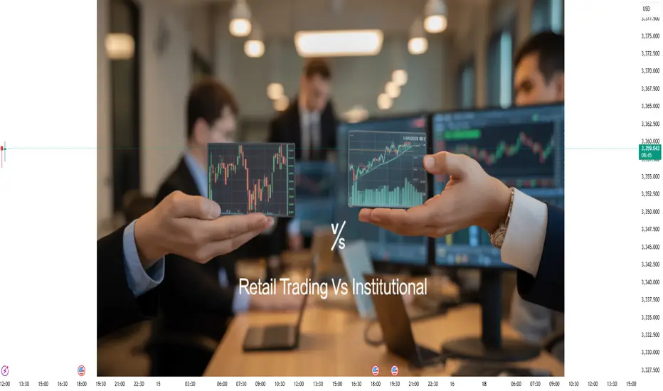
Retail vs Institutional Trading1. Introduction
In financial markets, traders can be broadly categorized into two groups: retail traders and institutional traders. While both operate in the same markets—stocks, forex, commodities, derivatives, cryptocurrencies—their goals, resources, and impact differ significantly.
Think of it like a chess game:
Retail traders are like passionate hobbyists, playing with personal strategies, smaller capital, and limited tools.
Institutional traders are like grandmasters with advanced chess engines, big teams, and massive resources.
Understanding the differences between these two groups is crucial for anyone involved in trading because:
It helps retail traders set realistic expectations.
It reveals how market moves are often driven by institutional flows.
It allows traders to align their strategies with the "big money" rather than fighting against it.
2. Defining the Players
Retail Traders
Who they are: Individual traders using their own capital to trade.
Examples: You, me, the average person with a brokerage account.
Capital size: Typically from a few hundred to a few hundred thousand dollars.
Trading style: Often short-term speculation, swing trading, or occasional long-term investing.
Motivation: Profit, financial freedom, hobby, or passive income.
Institutional Traders
Who they are: Professional traders working for large organizations, handling pooled funds.
Examples: Hedge funds, mutual funds, pension funds, banks, proprietary trading firms.
Capital size: Millions to billions of dollars.
Trading style: Long-term positions, algorithmic trading, arbitrage, high-frequency trading.
Motivation: Generate consistent returns for clients/investors, maintain market share, and manage risk.
3. Key Differences Between Retail & Institutional Trading
Aspect Retail Trading Institutional Trading
Capital Small, personal funds Huge pooled funds
Execution speed Slower, via broker platforms Ultra-fast, often via direct market access
Tools & technology Basic charting tools, retail brokers Advanced analytics, proprietary algorithms
Market impact Negligible Can move markets significantly
Risk tolerance Usually higher (due to smaller size) Often lower per trade but diversified
Regulations Fewer compliance rules Strict regulatory oversight
Information access Public data, delayed feeds Direct market data, insider networks (legal)
Strategy type Swing/day trading, small-scale strategies Large-scale arbitrage, hedging, portfolio balancing
4. Trading Infrastructure & Technology
Retail
Uses broker platforms like Zerodha, Upstox, Robinhood, E*TRADE.
Relies on charting software (TradingView, MetaTrader).
Order execution passes through multiple intermediaries, adding milliseconds or seconds of delay.
Limited access to Level 2 data and dark pool information.
Institutional
Uses Direct Market Access (DMA), bypassing middlemen.
Employs co-location — placing servers physically close to exchange data centers to reduce latency.
Custom-built AI-driven trading algorithms.
Access to Bloomberg Terminal, Reuters Eikon—costing thousands of dollars a month.
5. Market Impact
Retail Traders’ Impact
Individually, they have minimal effect on price.
Collectively, they can cause temporary market surges—e.g., GameStop 2021 short squeeze.
Often act as liquidity providers for institutional strategies.
Institutional Traders’ Impact
Can move prices by large orders.
Use order slicing (Iceberg Orders) to hide trade size.
Influence market sentiment through research, investment reports, and large portfolio shifts.
6. Trading Strategies
Retail Strategies
Day Trading – Quick in-and-out trades within the same day.
Swing Trading – Holding for days or weeks based on technical setups.
Trend Following – Buying in uptrends, selling in downtrends.
Breakout Trading – Entering when price breaches support/resistance.
Options Trading – Buying calls/puts for leveraged moves.
Copy Trading – Following successful traders’ trades.
Institutional Strategies
Algorithmic Trading – Automated, high-speed trade execution.
Market Making – Providing liquidity by quoting buy and sell prices.
Arbitrage – Exploiting price differences between markets.
Quantitative Strategies – Using statistical models for predictions.
Index Fund Management – Matching market indexes like S&P 500.
Hedging & Risk Management – Using derivatives to protect portfolios.
7. Advantages & Disadvantages
Retail Advantages
Flexibility: No need to report to clients.
Ability to take high-risk/high-reward bets.
Can enter/exit positions quickly due to small size.
Niche opportunities—small-cap stocks, micro trends.
Retail Disadvantages
Lack of insider or early information.
Higher transaction costs (relative to trade size).
Emotional trading—fear & greed affect decisions.
Lower technology access.
Institutional Advantages
Massive capital for diversification.
Best technology, research, and execution speeds.
Influence over market movements.
Access to private deals (private placements, IPO allocations).
Institutional Disadvantages
Large orders can move the market against them.
Regulatory and compliance burden.
Slower decision-making (bureaucracy).
Public scrutiny.
8. Regulatory Environment
Retail Traders:
Must follow general market rules set by SEBI (India), SEC (US), FCA (UK), etc.
Brokers are regulated; traders themselves are less scrutinized unless committing fraud.
Institutional Traders:
Heavily monitored by regulators.
Must follow reporting rules, such as 13F filings in the US.
Must ensure compliance with anti-money laundering (AML) and know-your-customer (KYC) laws.
9. Psychological Factors
Retail
Driven by emotions, social media hype, and news.
Prone to FOMO (Fear of Missing Out) and panic selling.
Often lack structured trading plans.
Institutional
Decisions made by teams, not individuals.
Uses risk-adjusted returns as a guiding principle.
Employs psychologists and behavioral finance experts to reduce bias.
10. Case Studies
GameStop 2021 – Retail Power
Retail traders on Reddit’s WallStreetBets caused a short squeeze.
Institutional short-sellers lost billions.
Showed that coordinated retail action can disrupt markets temporarily.
Flash Crash 2010 – Algorithmic Impact
Institutional algorithmic trading caused rapid market drops and rebounds.
Retail traders were mostly spectators.
Final Thoughts
Retail and institutional traders are two sides of the same market coin.
Retail traders bring diversity and liquidity, while institutional traders bring stability and efficiency—most of the time.
For retail traders, the key is to stop fighting institutional flows and instead follow their footprints. By understanding where big money is moving and aligning with it, retail traders can dramatically improve their odds of success.
In essence:
Institutional traders are the elephants in the market jungle.
Retail traders are the birds — smaller, more agile, able to grab quick opportunities the elephants can’t.
Economic Impact on Markets Introduction
Financial markets don’t move in isolation — they are deeply connected to the health and direction of the global and domestic economy. Every trader, whether in equities, commodities, currencies, or bonds, must understand that prices reflect not only company fundamentals or technical chart patterns but also broader economic forces.
Economic events and indicators act like weather reports for the market: they give traders a forecast of potential sunny growth or stormy recessions. This understanding allows traders to anticipate moves, manage risks, and identify opportunities.
In this guide, we’ll explore how economic factors impact markets, the key indicators to monitor, historical examples, and trading strategies to navigate different economic environments.
1. The Relationship Between Economy and Markets
The economy and markets are intertwined through several mechanisms:
Corporate Earnings Connection – A growing economy increases consumer spending and corporate profits, pushing stock prices higher.
Liquidity & Credit Cycle – Economic booms encourage lending, while slowdowns make credit expensive, impacting investments.
Risk Appetite – In good times, investors embrace risk; in downturns, they flock to safe assets like gold or government bonds.
Globalization Effects – Economic changes in one major country (e.g., the U.S., China) can ripple into global markets via trade, currency flows, and commodities.
Think of the market as a mirror of economic sentiment — sometimes slightly distorted by speculation, but largely reflecting real economic conditions.
2. Major Economic Indicators That Move Markets
Traders watch a set of macro indicators to gauge economic strength or weakness. These numbers often trigger sharp price moves.
2.1 GDP (Gross Domestic Product)
Definition: The total value of goods and services produced in a country.
Impact: Strong GDP growth signals economic expansion — bullish for stocks, bearish for bonds (due to potential rate hikes).
Example: U.S. Q2 2021 GDP growth of 6.7% boosted cyclical stocks like banks and industrials.
2.2 Inflation Data (CPI, WPI, PPI)
Consumer Price Index (CPI): Measures retail price changes.
Wholesale Price Index (WPI): Measures wholesale market price changes.
Producer Price Index (PPI): Measures production cost changes.
Impact: High inflation often prompts central banks to raise interest rates, which can hurt equity markets but benefit commodities.
Example: India’s CPI rising above 7% in 2022 led to RBI rate hikes and a correction in Nifty.
2.3 Employment Data
Non-Farm Payrolls (U.S.): Key job creation figure.
Unemployment Rate: Measures the percentage of jobless workers.
Impact: Strong job growth indicates economic health but can lead to inflationary pressures.
Example: U.S. unemployment dropping to 3.5% in 2019 fueled Fed tightening.
2.4 Interest Rates (Repo, Fed Funds Rate)
Central banks adjust rates to control inflation and stimulate or slow the economy.
Low rates encourage borrowing → boosts markets.
High rates slow growth → bearish for stocks, bullish for the currency.
2.5 Trade Balance & Currency Data
Surplus boosts domestic currency; deficit weakens it.
Currencies directly impact exporters/importers and global market flows.
2.6 PMI (Purchasing Managers’ Index)
Above 50 = expansion; below 50 = contraction.
Often moves manufacturing stocks.
3. Channels Through Which Economy Impacts Markets
3.1 Corporate Earnings Channel
Economic growth → higher sales → better earnings → higher stock valuations.
3.2 Consumer Spending & Confidence
Economic stability makes consumers spend more, benefiting retail, auto, and travel sectors.
3.3 Investment & Credit Flow
Low interest rates make borrowing cheaper for businesses, boosting capital investments.
3.4 Currency Valuation
A strong economy strengthens the currency, benefiting importers but hurting exporters.
3.5 Commodity Prices
Economic booms increase demand for oil, metals, and agricultural products.
4. Sectoral Impacts of Economic Conditions
4.1 During Economic Expansion
Winners: Cyclical sectors (banks, autos, infrastructure, luxury goods)
Laggards: Defensive sectors (FMCG, utilities) underperform relative to cyclical stocks.
4.2 During Economic Slowdown
Winners: Defensive sectors (healthcare, utilities, consumer staples)
Laggards: Cyclical sectors, high-debt companies.
4.3 High Inflation Environment
Winners: Commodity producers (metals, energy)
Laggards: Bond markets, growth stocks.
5. Historical Examples of Economic Impact on Markets
5.1 Global Financial Crisis (2008)
Triggered by U.S. housing collapse & credit crunch.
Nifty 50 fell over 50%.
Central banks cut rates to near zero.
5.2 COVID-19 Pandemic (2020)
GDP contraction globally.
Sharp sell-off in March 2020, followed by a massive rally due to stimulus.
Tech and pharma outperformed due to remote work & healthcare demand.
5.3 2022 Inflation & Rate Hikes
Surging commodity prices + supply chain disruptions.
Fed & RBI aggressive tightening → market volatility.
6. Trading Strategies for Different Economic Scenarios
6.1 Expansion Phase
Strategy: Buy cyclical growth stocks, high-beta sectors, small caps.
Risk: Overheated valuations.
6.2 Peak Phase
Strategy: Rotate into defensive stocks, lock profits in high-growth positions.
6.3 Recession Phase
Strategy: Defensive stocks, gold, bonds, short-selling indices.
6.4 Recovery Phase
Strategy: Gradually add cyclical exposure, focus on undervalued growth plays.
7. Economic Events Traders Should Track
Monetary Policy Meetings (RBI, Fed, ECB)
Budget Announcements
Corporate Earnings Season
Global Trade Agreements
Geopolitical Tensions
8. Risk Management in Economic-Driven Markets
Stay Hedged: Use options or inverse ETFs.
Diversify: Across sectors and asset classes.
Set Stop Losses: Especially during high-volatility data releases.
Don’t Trade Blind: Always check the economic calendar before placing trades.
9. Final Thoughts
Economic forces are the engine driving market movement. A trader who understands GDP trends, inflation patterns, interest rate cycles, and sectoral dynamics can navigate markets more effectively than someone relying only on chart patterns.
Markets anticipate — they often move before economic reports confirm the trend. This means the most successful traders not only react to data but also position themselves ahead of it, using both macroeconomic insights and technical signals.

Smart Money Concepts (SMC) & Liquidity Trading1. Introduction
In financial markets, price does not move randomly — it’s influenced by the decisions of big players often called Smart Money. These players include institutional investors, hedge funds, prop firms, and high-frequency trading algorithms. Unlike retail traders, they have vast capital, deep research capabilities, and the ability to move markets.
Smart Money Concepts (SMC) is a modern trading framework that focuses on understanding how these institutions operate — where they enter, where they exit, and how they trap retail traders.
A related idea is Liquidity Trading, which explains how Smart Money hunts for liquidity — areas in the market where many buy/sell orders are clustered. The price often moves to these zones before reversing.
In short:
Retail traders follow indicators and news.
Smart Money follows liquidity and order flow.
2. The Core Principles of Smart Money Concepts
SMC revolves around understanding the footprints left by institutional traders.
2.1 Market Structure
Market structure refers to how price moves in swings — forming highs and lows.
Bullish Structure: Higher Highs (HH) & Higher Lows (HL)
Bearish Structure: Lower Highs (LH) & Lower Lows (LL)
Structure Break (BOS): When price violates the previous high/low — signaling a potential trend change.
Change of Character (CHOCH): Early sign of trend reversal when price breaks the first structural level in the opposite direction.
📌 Why it matters in SMC:
Smart Money often shifts from accumulation to distribution phases through structure breaks. If you can read structure, you can anticipate reversals.
2.2 Order Blocks
An Order Block is the last bullish or bearish candle before a strong price move in the opposite direction, usually caused by institutional order placement.
Bullish Order Block (B-OB): Last down candle before price surges upward.
Bearish Order Block (B-OB): Last up candle before price drops.
📌 Why it matters:
Institutions leave these “footprints” because their large orders cannot be filled instantly. Price often revisits these zones to fill unexecuted orders before moving further.
2.3 Liquidity Pools
Liquidity pools are areas where many stop-losses or pending orders are gathered.
Buy-Side Liquidity (BSL): Above swing highs where buy stop orders and short stop-losses sit.
Sell-Side Liquidity (SSL): Below swing lows where sell stop orders and long stop-losses sit.
📌 Why it matters:
Smart Money drives price into these pools to trigger stop orders and gain enough liquidity to enter or exit large positions.
2.4 Fair Value Gaps (FVG) / Imbalances
A Fair Value Gap is a price imbalance caused when market moves rapidly, leaving a gap in the price structure (often between candle wicks).
📌 Why it matters:
Price often returns to fill these gaps before continuing the main trend, as Smart Money prefers balanced price action.
2.5 The “Smart Money Cycle”
The market typically moves in this cycle:
Accumulation – Institutions quietly build positions at key zones.
Manipulation (Liquidity Grab) – Price fakes out retail traders by hitting stop losses or false breakouts.
Distribution (Mark-up/Mark-down) – The true move begins as Smart Money pushes price strongly in the intended direction.
3. Liquidity Trading in Detail
Liquidity trading focuses on identifying where liquidity is and predicting how price will move to capture it.
3.1 Why Liquidity Matters
Large orders cannot be executed without enough liquidity. Institutions need retail traders' orders to fill their positions.
Example:
If a hedge fund wants to go long, they need sellers to provide liquidity.
They might push the price down first, triggering stop-losses of buyers, to gather those sell orders before pushing price up.
3.2 Types of Liquidity
Resting Liquidity:
Stop-losses above/below swing highs/lows.
Pending limit orders at support/resistance.
Dynamic Liquidity:
Orders entering the market as price moves (market orders).
Session Liquidity:
High liquidity periods like London Open, New York Open.
3.3 Liquidity Grab (Stop Hunt)
A liquidity grab is when price briefly moves past a key level to trigger orders before reversing.
Example:
Retail sees resistance at 1.2000 in EUR/USD.
Price spikes to 1.2005 (triggering breakout buys and stop-losses of shorts).
Immediately reverses to 1.1950.
4. Combining SMC & Liquidity Trading
The real power comes when you merge SMC concepts with liquidity zones.
4.1 Step-by-Step Process
Identify Market Structure – Are we in bullish or bearish territory?
Mark Liquidity Zones – Where are the obvious highs/lows where orders cluster?
Spot Order Blocks – Look for institutional footprints.
Watch for Liquidity Grabs – Did price sweep a high/low?
Enter on Confirmation – Use BOS, CHOCH, or FVG fills for precise entries.
Manage Risk – Stop-loss just beyond liquidity sweep zones.
4.2 Example Trade
Context: Bullish trend on daily chart.
Liquidity Zone: Sell-side liquidity just below recent swing low.
Event: Price dips below swing low during London session (stop hunt), then aggressively pushes upward.
Entry: After BOS on 15-min chart.
Stop-loss: Below liquidity sweep low.
Target: Next buy-side liquidity pool above.
5. The Psychology Behind SMC
Institutions know retail traders:
Use obvious support/resistance.
Place stop-losses just beyond these zones.
Chase breakouts without confirmation.
Smart Money uses this predictability to engineer liquidity events — moving price to trap one side before reversing.
📌 Key Insight:
Price doesn’t move because of “magic” — it moves because Smart Money needs liquidity to execute orders.
6. Common Mistakes Traders Make
Blindly Trading Order Blocks – Not all OBs are valid; context is crucial.
Ignoring Higher Timeframes – A valid OB on 5-min might be irrelevant in daily structure.
Confusing BOS with CHOCH – Leads to premature entries.
Not Waiting for Confirmation – Jumping in before liquidity is grabbed.
Overloading Indicators – SMC works best with a clean chart.
7. Advanced SMC & Liquidity Concepts
7.1 Mitigation Blocks
When price returns to an order block but doesn’t fully reverse — instead, it continues trend after partially “mitigating” the zone.
7.2 Internal & External Liquidity
External Liquidity: Major swing highs/lows visible to everyone.
Internal Liquidity: Smaller highs/lows inside larger moves.
Smart Money often sweeps internal liquidity first, then external liquidity.
7.3 Time & Price Theory
Certain times of day (e.g., London open) align with higher probability liquidity sweeps due to volume influx.
8. Practical Trading Plan Using SMC & Liquidity
8.1 Daily Preparation
Higher Timeframe Bias:
Identify daily & 4H market structure.
Mark Key Zones:
Liquidity pools, order blocks, FVGs.
Session Plan:
Anticipate liquidity grabs during London/NY opens.
8.2 Execution Rules
Wait for liquidity sweep.
Confirm with BOS or CHOCH.
Enter with minimal risk, aiming for 1:3+ R:R.
Exit at next liquidity pool.
8.3 Risk Management
Risk 1% per trade.
Stop-loss beyond liquidity grab.
Use partial profit-taking at mid-targets.
9. Why SMC Outperforms Traditional Strategies
Focuses on why price moves, not just what price does.
Aligns trading with the biggest players in the market.
Avoids fakeouts by understanding liquidity grabs.
10. Final Thoughts
Smart Money Concepts & Liquidity Trading are not “magic tricks.”
They’re a lens to view the market’s true mechanics — the interplay of institutional demand and retail supply.
When mastered:
You stop fearing stop hunts — you anticipate them.
You stop guessing — you read the market’s intent.
You trade with the big players, not against them.

Part 8 Trading Master ClassCommon Mistakes to Avoid
Holding OTM options too close to expiry hoping for a miracle.
Selling naked calls without understanding unlimited risk.
Over-leveraging with too many contracts.
Ignoring commissions and slippage.
Not adjusting positions when market changes.
Practical Tips for Success
Backtest strategies on historical data.
Start with paper trading before using real money.
Track your trades in a journal.
Combine technical analysis with options knowledge.
Trade liquid options with tight bid-ask spreads.

Part11 Trading Master ClassOption Chain Key Terms
Let’s go deep into each term one by one.
Strike Price
The predetermined price at which you can buy (Call) or sell (Put) the underlying asset if you exercise the option.
Every expiry has multiple strike prices — some above the current market price, some below.
Example:
If NIFTY is at 19,500:
19,500 Strike → ATM (At The Money)
19,600 Strike → OTM (Out of The Money) Call, ITM (In The Money) Put
19,400 Strike → ITM Call, OTM Put
Expiry Date
The last trading day for the option. After this date, the contract expires worthless if not exercised.
In India:
Index options (like NIFTY, BANKNIFTY) → Weekly expiries + Monthly expiries
Stock options → Monthly expiries
Call Option (CE)
Gives you the right (not obligation) to buy the underlying at the strike price.
Traders buy calls when they expect the price to rise.
Put Option (PE)
Gives you the right (not obligation) to sell the underlying at the strike price.
Traders buy puts when they expect the price to fall.

Option Chain Terms1. Introduction: What is an Option Chain?
An Option Chain (also called an options matrix) is like a detailed menu for all the available Call and Put options of a particular underlying asset (such as a stock, index, or commodity) for different strike prices and expiry dates.
If you’re a trader, the option chain is where you see all the numbers that decide your trading choices — prices, volumes, open interest, and Greeks.
Think of it as the cockpit of an airplane — lots of data, but if you know what each dial means, you can navigate smoothly.
Example:
If you open the NSE India website and look at the NIFTY Option Chain, you’ll see something like:
Strike Price CALL LTP CALL OI PUT LTP PUT OI
19500 ₹250 1,20,000 ₹15 80,000
19600 ₹180 95,000 ₹25 90,000
This is a simplified snapshot — in reality, there are more columns like bid-ask prices, implied volatility, and Greeks.
2. Core Sections of an Option Chain
An option chain is split into two halves:
Left Side: Call options (bullish contracts)
Right Side: Put options (bearish contracts)
Middle: Strike Prices (common to both)
Here’s how the layout looks visually:
markdown
Copy
Edit
CALL DATA | STRIKE PRICE | PUT DATA
-----------------------------------------------
OI Chg OI LTP IV | 19500 | IV LTP Chg OI OI
OI Chg OI LTP IV | 19600 | IV LTP Chg OI OI
3. Option Chain Key Terms
Let’s go deep into each term one by one.
3.1 Strike Price
The predetermined price at which you can buy (Call) or sell (Put) the underlying asset if you exercise the option.
Every expiry has multiple strike prices — some above the current market price, some below.
Example:
If NIFTY is at 19,500:
19,500 Strike → ATM (At The Money)
19,600 Strike → OTM (Out of The Money) Call, ITM (In The Money) Put
19,400 Strike → ITM Call, OTM Put
3.2 Expiry Date
The last trading day for the option. After this date, the contract expires worthless if not exercised.
In India:
Index options (like NIFTY, BANKNIFTY) → Weekly expiries + Monthly expiries
Stock options → Monthly expiries
3.3 Call Option (CE)
Gives you the right (not obligation) to buy the underlying at the strike price.
Traders buy calls when they expect the price to rise.
3.4 Put Option (PE)
Gives you the right (not obligation) to sell the underlying at the strike price.
Traders buy puts when they expect the price to fall.
3.5 LTP (Last Traded Price)
The most recent price at which the option contract traded.
Reflects the current market value of that option.
3.6 Bid Price & Ask Price
Bid Price: Maximum price buyers are willing to pay.
Ask Price: Minimum price sellers are willing to accept.
The gap between them is called the Bid-Ask Spread.
3.7 Bid Quantity & Ask Quantity
Bid Quantity: Number of contracts buyers want to purchase at the bid price.
Ask Quantity: Number of contracts sellers are offering at the ask price.
3.8 Volume
Total number of contracts traded during the current trading session.
High volume indicates strong interest and liquidity.
3.9 Open Interest (OI)
Total number of outstanding contracts that haven’t been closed or squared off.
Shows market positioning:
High OI in calls → Bearish or range-bound expectation.
High OI in puts → Bullish or range-bound expectation.
3.10 Change in Open Interest (Chg OI)
How much OI has increased or decreased from the previous session.
Used to detect fresh positions or unwinding.
3.11 Implied Volatility (IV)
Market’s expectation of future volatility.
Higher IV → Option premiums become expensive.
Lower IV → Options are cheaper.
3.12 Greeks in the Option Chain
Greeks measure how sensitive the option price is to changes in market factors:
Delta → Price change sensitivity to the underlying asset.
Gamma → Rate of change of Delta.
Theta → Time decay rate of the option price.
Vega → Sensitivity to changes in volatility.
Rho → Sensitivity to interest rate changes.
3.13 ATM, ITM, and OTM
ATM (At The Money): Strike price is equal to the current price.
ITM (In The Money): Option has intrinsic value.
OTM (Out of The Money): Option has no intrinsic value (only time value).
3.14 Premium
The price you pay to buy an option.
Premium = Intrinsic Value + Time Value.
3.15 Break-Even Point
Price level at which your option trade starts becoming profitable.
3.16 PCR (Put-Call Ratio)
Formula: PCR = Put OI / Call OI
High PCR (>1) → Bullish sentiment.
Low PCR (<1) → Bearish sentiment.
4. How to Read the Option Chain
Reading an option chain is about spotting where traders are placing their bets.
Step-by-step:
Identify ATM Strike.
See highest OI in Calls and Puts — this shows resistance and support levels.
Look at Change in OI to spot fresh activity.
Check IV movement for volatility expectations.
Use Greeks for risk assessment.
Example Analysis:
NIFTY at 19,500
Highest Call OI: 19,800 (Resistance)
Highest Put OI: 19,400 (Support)
PCR = 1.2 → Mildly bullish
5. Practical Use Cases
Finding Support & Resistance:
Highest Put OI → Support
Highest Call OI → Resistance
Spotting Breakouts:
Sudden drop in Call OI at resistance → Possible breakout.
Volatility Trading:
High IV → Consider selling options.
Low IV → Consider buying options.
6. Advanced Option Chain Insights
Long Buildup: Price ↑, OI ↑ → Bullish.
Short Buildup: Price ↓, OI ↑ → Bearish.
Short Covering: Price ↑, OI ↓ → Bullish reversal.
Long Unwinding: Price ↓, OI ↓ → Bearish reversal.
7. Common Mistakes to Avoid
Ignoring IV before entering trades.
Reading OI without considering price movement.
Not adjusting for upcoming news or events.
Trading illiquid strikes with wide bid-ask spreads.
8. Conclusion
An option chain is not just a table of numbers — it’s a real-time X-ray of trader sentiment.
By understanding every term — from LTP to IV, from Delta to PCR — you can turn raw data into actionable insights.
Private vs. Public Sector Banks 1. Introduction
Banks are the backbone of any economy. They are not just safe houses for our money; they act as credit suppliers, payment facilitators, and growth enablers for individuals, businesses, and governments.
In India — and in most countries — banks are broadly divided into public sector banks (PSBs) and private sector banks (Pvt banks). While both serve the same core purpose of financial intermediation, their ownership, management, operational style, and even their customer experience differ significantly.
Understanding Private vs. Public Sector Banks is not just an academic exercise — it’s crucial for:
Investors who want to choose where to put their money.
Job seekers deciding between PSU banking careers and private sector opportunities.
Customers looking for the best mix of safety, returns, and service quality.
Policy makers trying to design financial inclusion and credit growth policies.
2. What are Public Sector Banks?
Definition:
A public sector bank is a bank where the majority stake (more than 50%) is held by the government — either the central government, state government, or both.
Key Characteristics:
Ownership: Government-controlled.
Governance: Board of directors often includes government nominees.
Mandate: Balances commercial profitability with social objectives like financial inclusion.
Funding & Support: Can access government capital infusion during crises.
Regulation: Supervised by the Reserve Bank of India (RBI), but also influenced by government policies.
Examples in India:
State Bank of India (SBI) – India’s largest bank.
Punjab National Bank (PNB)
Bank of Baroda (BoB)
Canara Bank
Union Bank of India
Globally, similar examples exist — such as Bank of China or Royal Bank of Scotland (in the past).
3. What are Private Sector Banks?
Definition:
A private sector bank is owned and operated by private individuals or corporations, where the majority of shares are held by private stakeholders.
Key Characteristics:
Ownership: Private promoters and institutional investors.
Governance: Professional boards, often with market-driven incentives.
Mandate: Primarily driven by profitability, efficiency, and shareholder returns.
Customer Orientation: More aggressive in marketing, product innovation, and digital adoption.
Regulation: Supervised by the RBI but largely free from direct government operational control.
Examples in India:
HDFC Bank – India’s largest private sector bank.
ICICI Bank
Axis Bank
Kotak Mahindra Bank
Yes Bank
Globally, examples include JPMorgan Chase, HSBC, and Citibank.
4. Historical Context in India
The distinction between public and private banks in India is rooted in policy decisions.
Pre-Nationalisation Era (Before 1969)
Most banks were privately owned, often run by business families.
Credit was concentrated in urban areas; rural India had limited access.
Frequent bank failures occurred due to poor regulation.
Nationalisation (1969 & 1980)
In 1969, Prime Minister Indira Gandhi nationalised 14 major private banks.
In 1980, 6 more banks were nationalised.
Goal: Direct credit to agriculture, small industries, and backward areas.
Result: PSBs became dominant — controlling over 90% of banking business.
Post-Liberalisation (1991 onwards)
New private banks like HDFC Bank, ICICI Bank, and Axis Bank emerged.
RBI allowed foreign banks to operate more freely.
PSB dominance declined, but they still remain vital for rural outreach.
5. Ownership & Governance Differences
Feature Public Sector Banks Private Sector Banks
Ownership Majority (>50%) by Government Majority by private individuals/institutions
Board Control Government nominees, political influence possible Independent/professional management
Capital Infusion Often from government budget Raised from private investors or markets
Accountability Parliament, RBI, and public scrutiny Shareholders and RBI
6. Objectives & Mandates
Public Sector Banks:
Financial inclusion
Support for agriculture, MSMEs, and infrastructure
Government welfare scheme implementation (e.g., Jan Dhan Yojana)
Stability in rural credit supply
Private Sector Banks:
Profitability and market share growth
Product innovation and niche targeting
Maximizing shareholder returns
Efficiency and cost optimization
7. Operational Style & Customer Service
Public Sector Banks:
Tend to have larger rural branch networks.
Service quality can vary; bureaucratic processes are common.
Product range is adequate but less aggressive in innovation.
Loan approvals may be slower due to multiple verification layers.
Examples: SBI’s YONO app shows digital adaptation, but rollout is slower.
Private Sector Banks:
More urban-centric (though expanding into semi-urban and rural).
Aggressive in customer acquisition and cross-selling.
Loan approvals and service delivery are often faster.
Early adopters of technology — e.g., HDFC Bank’s mobile banking, ICICI’s iMobile app.
More flexible in product design.
8. Technology Adoption
Aspect Public Sector Banks Private Sector Banks
Digital Banking Gradual adoption; integration with legacy systems slows pace Rapid adoption; cloud & AI-powered tools
Customer Onboarding Often in-branch, with KYC paperwork Instant account opening via apps
Innovation Moderate; often after private sector pioneers Aggressive; lead in UPI, API banking
Example: HDFC Bank was among the first in India to launch a net banking platform in 1999. PSBs followed years later.
9. Financial Performance & Profitability
Private banks generally outperform PSBs in:
Return on Assets (RoA)
Return on Equity (RoE)
Net Interest Margin (NIM)
PSBs, however, have:
Larger deposit base due to government trust factor.
Wider financial inclusion footprint.
Example (FY24 Data, approx.):
HDFC Bank RoA: ~2.0%
SBI RoA: ~0.9%
HDFC Bank NIM: ~4.1%
SBI NIM: ~3.2%
10. Risk & NPA Levels
Public Sector Banks:
Historically higher Non-Performing Assets (NPAs) due to priority sector lending, political interference, and legacy loans.
Government recapitalises them when losses mount.
Private Sector Banks:
More selective in lending.
Lower NPA ratios on average.
But risk exists — e.g., Yes Bank crisis in 2020.
11. Role in the Economy
Public Sector Banks:
Act as financial shock absorbers.
Support government borrowing and welfare distribution.
Primary channel for rural development finance.
Private Sector Banks:
Drive innovation in payments, digital finance, and wealth management.
Cater to affluent and corporate clients more aggressively.
Attract foreign investment in India’s banking sector.
12. Global Comparisons
In countries like China, public banks dominate (e.g., Industrial and Commercial Bank of China).
In the US, most banks are privately owned, with government stepping in during crises (e.g., 2008 bailout).
India’s model is hybrid — both sectors coexist, serving different but overlapping needs.
Conclusion
The Public vs. Private Sector Bank debate is not about which is “better” in an absolute sense — both are indispensable pillars of the financial system.
Public sector banks ensure financial inclusion, rural development, and stability, while private sector banks drive efficiency, innovation, and competitive service.
For customers, the best choice often depends on priorities:
If trust, safety, and rural access are key — PSBs shine.
If speed, digital ease, and product innovation matter — private banks lead.
For the economy, a balanced dual banking ecosystem ensures stability and progress.

Mastering the Art of Risk Management in Trading 1. Introduction: Why Risk Management is the Heart of Trading
Trading is not about making big profits quickly — it’s about staying in the game long enough to let your edge work for you.
Think of trading like a professional sport. Skill matters, but survival matters more. Even the world’s best traders lose trades; what separates them from amateurs is how they manage those losses.
In simple terms:
Good trading without risk management = gambling.
Average trading with strong risk management = long-term success.
Warren Buffett’s famous rules apply perfectly here:
Don’t lose money.
Never forget rule #1.
2. Core Principles of Risk Management
Before we go deep into strategies, let’s lock in the foundation.
2.1 Risk is Inevitable
Every trade carries risk. The goal is not to avoid it but to control its size and impact.
2.2 Asymmetry in Trading
A 50% loss requires a 100% gain to break even. This means avoiding large drawdowns is far more important than chasing big wins.
Loss % Required Gain to Recover
10% 11.1%
25% 33.3%
50% 100%
75% 300%
2.3 Risk per Trade
Most professional traders risk 0.5%–2% of their account per trade.
This ensures no single bad trade can destroy the account.
3. The Psychology of Risk
Risk management is not just math — it’s deeply psychological.
Loss Aversion Bias: Humans feel losses twice as strongly as gains. This can push traders into revenge trading.
Overconfidence Bias: Winning streaks can lead to oversized positions.
Fear of Missing Out (FOMO): Chasing trades without proper entry rules increases risk.
A great risk management system removes emotional decision-making by setting clear, mechanical rules.
4. Position Sizing: The Risk Control Lever
Position sizing determines how much capital to put into a trade. Even if your strategy is perfect, bad sizing can blow up your account.
4.1 Fixed Fractional Method
Risk a fixed % of capital per trade.
Example: If account = ₹10,00,000 and risk = 1% → Risk per trade = ₹10,000.
If Stop Loss = ₹50 away from entry, position size = ₹10,000 ÷ ₹50 = 200 shares.
4.2 Volatility-Based Position Sizing
Adjust position size according to the volatility of the asset (ATR – Average True Range).
If ATR = ₹25 and your risk budget = ₹5,000, position size = ₹5,000 ÷ ₹25 = 200 shares.
4.3 Kelly Criterion (Advanced)
Maximizes capital growth based on win rate & reward/risk ratio.
Formula: K% = W – (1 – W) / R
Where:
W = Win probability
R = Reward/Risk ratio
Caution: Kelly is aggressive; use fractional Kelly for real trading.
5. Stop Loss Strategies: Your Safety Net
A stop loss is not a sign of weakness — it’s a shield.
5.1 Fixed Stop Loss
Predefined point in price where you exit.
5.2 Volatility Stop Loss
Adjust stop distance using ATR to account for market noise.
5.3 Time-Based Stop
Exit after a fixed time if the trade hasn’t moved in your favor.
5.4 Trailing Stop
Moves with price in your favor to lock in profits.
Golden Rule: Place stops based on market structure, not emotions.
6. Reward-to-Risk Ratio (RRR)
The RRR tells you how much you stand to gain for every unit you risk.
Example:
Risk: ₹1000
Reward: ₹3000
RRR = 3:1 → Even a 40% win rate is profitable.
High RRR trades allow more losers than winners while staying profitable.
7. Diversification & Correlation Risk
7.1 Asset Diversification
Avoid putting all capital into one asset or sector.
7.2 Correlation Risk
If you buy Nifty futures and Bank Nifty futures, you’re effectively doubling your risk because they move together.
8. Risk Management for Different Trading Styles
8.1 Day Trading
Keep daily loss limits (e.g., 3% of capital).
Avoid revenge trading after a loss.
8.2 Swing Trading
Use wider stops to allow for multi-day fluctuations.
Position sizing becomes even more critical.
8.3 Options Trading
Risk can be higher due to leverage.
Always calculate max loss before entering.
9. Risk Management Tools
ATR Indicator – For volatility-based stops.
Position Size Calculators – To control exposure.
Heat Maps & Correlation Tools – To avoid overexposure.
Journaling Software – To track mistakes.
10. Risk-Adjusted Performance Metrics
Professional traders measure performance relative to risk taken.
Sharpe Ratio – Risk-adjusted returns.
Sortino Ratio – Focuses on downside volatility.
Max Drawdown – Largest account drop during a period.
11. Building a Personal Risk Management Plan
Your plan should cover:
Max % of capital risked per trade.
Max daily/weekly loss limit.
Position sizing rules.
Stop loss & target placement method.
Diversification guidelines.
Rules for scaling in/out.
Plan for handling drawdowns.
12. Advanced Concepts
12.1 Portfolio Heat
Sum of all open trade risks; keep it below a set % of account.
12.2 Value at Risk (VaR)
Estimates the max expected loss over a time frame.
12.3 Stress Testing
Simulate worst-case scenarios (e.g., gap downs, black swans).
Conclusion: Risk Management is Your Superpower
In trading, capital is ammunition. Risk management ensures you never run out of bullets before the big opportunities arrive.
Mastering it is not optional — it’s the difference between a short-lived hobby and a long-term career.