Private vs Public Banks: Role in the Indian Trading Market1. Overview of Public and Private Banks in India
1.1 Public Sector Banks (PSBs)
Public sector banks are those where the majority ownership (more than 50%) lies with the Government of India. Examples include the State Bank of India (SBI), Punjab National Bank (PNB), Bank of Baroda, and Canara Bank. PSBs dominate the Indian banking sector in terms of branch network, assets under management (AUM), and reach, particularly in rural and semi-urban regions.
Key Characteristics of PSBs:
Government-owned with social and development mandates.
Conservative in risk-taking.
Large customer base across rural and urban India.
Often involved in policy-driven lending and financial inclusion schemes.
1.2 Private Sector Banks (PVBs)
Private banks, such as HDFC Bank, ICICI Bank, Axis Bank, and Kotak Mahindra Bank, are owned predominantly by private shareholders. These banks are known for customer-centric approaches, high efficiency, and greater use of technology. They have grown rapidly in the last two decades and now have significant influence in retail, corporate, and investment banking.
Key Characteristics of PVBs:
Privately owned with profit-driven motives.
Higher risk appetite and innovative products.
Focused on urban and semi-urban populations.
Advanced technological adoption and superior customer service.
2. Role in the Indian Trading Market
The Indian trading market comprises equities, commodities, derivatives, forex, and bond markets. Both private and public banks play distinct roles in facilitating trading activities, investment, and capital flow.
2.1 Providing Capital and Liquidity
PSBs: They are crucial in funding large-scale corporate and government projects, which indirectly impacts trading markets by providing liquidity and supporting corporate growth. PSBs often lend to companies whose stocks or bonds are actively traded in the market.
PVBs: These banks are more active in retail lending, margin finance, and funding startups or small-cap companies. By offering working capital, they help increase market participation and trading volumes.
2.2 Investment Banking and Market Operations
PSBs: Traditionally, PSBs have a limited role in high-risk investment banking activities. However, banks like SBI Capital Markets actively participate in primary market issuances (IPOs) and underwriting services, supporting capital formation.
PVBs: Private banks are more aggressive in equity and bond issuance, IPO management, advisory services, and mergers & acquisitions (M&A). They provide liquidity to the trading market and cater to institutional investors, contributing to market depth.
2.3 Facilitating Retail and Institutional Trading
Retail Market: Private banks lead in offering demat accounts, online trading platforms, and wealth management services, making trading accessible to individual investors. PSBs have been slower in digital adoption but still serve a large customer base with affordable services.
Institutional Market: PSBs dominate government securities (G-Secs) trading, large-scale corporate bonds, and interbank transactions, whereas PVBs are more flexible in providing structured products and derivatives to hedge risks in trading portfolios.
3. Technological Innovation and Trading Efficiency
3.1 Digital Platforms
PVBs: Banks like HDFC, ICICI, and Kotak Mahindra have pioneered digital banking solutions, including online trading, mobile apps, algorithmic trading support, and seamless payment gateways. These platforms enhance efficiency in stock, forex, and commodity markets.
PSBs: Although improving, public banks have traditionally lagged in adopting high-speed trading platforms. Their digital offerings are often centralized but less user-friendly for advanced traders.
3.2 Data Analytics and Market Insights
Private banks leverage big data analytics and AI-driven trading advisory, providing traders and investors with market insights, technical analysis, and risk management tools.
Public banks, while increasingly offering research services, focus mainly on policy-driven investment guidance and macroeconomic reports.
4. Risk Management and Market Stability
4.1 Risk Appetite
PSBs: Conservative lending and trading practices help maintain market stability, preventing excessive speculation. However, this may limit high-growth opportunities in trading markets.
PVBs: Their higher risk appetite fosters innovation and liquidity but may also contribute to volatility, especially in derivatives and structured products.
4.2 Crisis Management
PSBs: During market downturns, public banks play a stabilizing role by maintaining credit flow to companies and acting as government channels for economic stimulus.
PVBs: While they provide risk-mitigating tools like hedging products, their reliance on market-driven profits makes them vulnerable during severe market corrections.
5. Role in Government and Policy Initiatives
PSBs are instrumental in implementing government-backed schemes like MUDRA loans, priority sector lending (PSL), and disbursal of subsidies. These measures impact trading indirectly by enhancing disposable income and liquidity in the economy.
PVBs participate in policy initiatives selectively, often aligning with profit motives, such as facilitating corporate bond markets, IPO underwriting, and private wealth management.
6. Impact on Stock, Commodity, and Forex Markets
6.1 Equity Market
PSBs: Major institutional investors; provide long-term funding and participate in strategic equity investments. Their trading volume may be lower but stable.
PVBs: Retail-oriented and innovative products enhance equity market participation. They facilitate derivatives trading, margin financing, and high-frequency trading for active investors.
6.2 Commodity Market
PSBs: Serve as financing partners for commodity producers and importers, ensuring supply chain liquidity.
PVBs: Offer customized hedging solutions and online platforms for commodity trading, attracting active market participants.
6.3 Forex Market
PSBs: Dominant in external commercial borrowing (ECB), trade finance, and remittance services, crucial for forex stability.
PVBs: Provide competitive forex services, real-time trading, and risk management tools for businesses and individual traders.
7. Comparative Analysis: Public vs Private Banks
Aspect Public Sector Banks Private Sector Banks
Ownership Government Private
Risk Appetite Conservative Higher
Market Reach Nationwide, including rural Urban & semi-urban focused
Technology Adoption Moderate High
Retail Trading Support Limited digital services Advanced platforms & apps
Institutional Role Government & corporate Corporate & investment banking
Market Stability Stabilizing Liquidity enhancer, can be volatile
Financial Inclusion High Moderate
Trading Products Traditional bonds, G-Secs Derivatives, structured products, margin trading
8. Challenges and Opportunities
8.1 Challenges
PSBs: Legacy systems, NPA (Non-Performing Asset) issues, slower technological adoption, and bureaucratic decision-making hinder active participation in fast-paced trading markets.
PVBs: Exposure to market volatility, regulatory pressures, and high competition requires constant innovation to remain relevant in trading markets.
8.2 Opportunities
PSBs: Digital transformation, strategic partnerships with fintechs, and expanding advisory services can boost their trading market role.
PVBs: Expanding into rural markets, leveraging AI-driven trading analytics, and tapping government-backed schemes offer growth potential.
9. Conclusion
The roles of public and private banks in the Indian trading market are complementary rather than competitive. Public banks provide stability, government-backed funding, and long-term institutional support, making them pillars of the financial ecosystem. Private banks, in contrast, drive innovation, liquidity, and retail participation through advanced technology, flexible financial products, and customer-centric services.
Together, both sectors enhance market efficiency, capital formation, risk management, and investor confidence, ensuring the Indian trading market remains vibrant and robust. The future of India’s trading ecosystem will increasingly depend on how both public and private banks leverage technology, collaborate with fintechs, and balance risk with sustainable growth.
X-indicator

Part 2 Master Class of Intraday TradingCall and Put Options Explained
A Call Option gives the buyer the right to purchase an asset at a specific price (strike price) before or on the expiry date. Investors buy calls when they expect the asset’s price to rise. Conversely, a Put Option gives the buyer the right to sell the asset at the strike price, used when expecting a price fall. Sellers of options (writers) have obligations—call writers must sell, and put writers must buy if exercised. The interplay between call and put options allows for complex strategies, such as spreads and straddles. Understanding how both function is vital for predicting market direction and building profitable positions.

Part 1 Master Class of Intraday Trading Understanding the Concept of Options
Option trading involves financial contracts that give buyers the right, but not the obligation, to buy or sell an underlying asset—like a stock, index, or commodity—at a predetermined price within a specific period. The two main types are Call Options (buy rights) and Put Options (sell rights). Unlike owning shares directly, options let traders speculate on price movements with limited capital. The right to buy or sell comes at a cost known as the premium. Options are widely used for hedging, speculation, and income generation. Their value is influenced by factors such as volatility, time decay, and market sentiment. Understanding these dynamics helps traders manage risk and seize market opportunities efficiently.

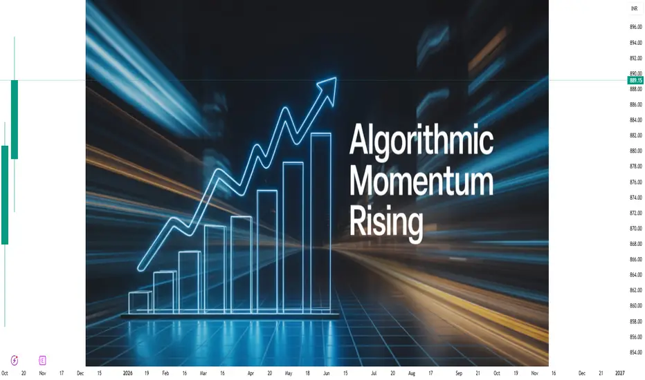
Algorithmic Momentum Trading1. Understanding Momentum in Financial Markets
Momentum trading is grounded in a simple behavioral finance principle: “trends tend to persist.” In other words, securities that have performed well in the past are likely to continue performing well in the near future, and vice versa for underperforming assets. Momentum can be measured in various ways, such as:
Price-based momentum: Observing past price performance over specific periods (e.g., 1 month, 3 months, 6 months).
Volume-based momentum: Using trading volume spikes as a signal of growing market interest.
Volatility-based momentum: Identifying assets experiencing strong directional moves with low resistance, indicating strong trend potential.
Momentum traders aim to capitalize on these trends by buying assets showing upward momentum and selling or shorting those with downward momentum. The key challenge, however, lies in accurately identifying trends early and managing the risks associated with reversals.
2. Role of Algorithms in Momentum Trading
The traditional momentum trading approach relied heavily on manual observation of charts, price patterns, and technical indicators. However, the advent of algorithmic trading has revolutionized this process. Algorithmic momentum trading uses computer programs to detect trends and execute trades automatically. Key advantages include:
Speed: Algorithms can process market data and execute trades in milliseconds, far faster than humans.
Consistency: Algorithms eliminate emotional bias, ensuring a disciplined application of the momentum strategy.
Data handling: They can monitor multiple assets, markets, and time frames simultaneously, which would be impossible manually.
Scalability: High-frequency trading (HFT) and large portfolios can be managed efficiently with algorithmic systems.
In essence, algorithmic momentum trading combines the predictive power of momentum strategies with the speed and precision of automated systems.
3. Core Momentum Trading Strategies
Algorithmic momentum trading is not a single strategy but a collection of approaches that exploit market trends. Some widely used strategies include:
3.1 Price Momentum Strategy
This strategy identifies assets that have been appreciating over a recent period. The algorithm monitors price changes over fixed intervals (e.g., daily, weekly, monthly) and generates buy signals when prices exceed certain thresholds. Typical indicators include:
Moving Averages (MA): Assets trading above their short-term moving average (e.g., 50-day MA) are considered bullish.
Relative Strength Index (RSI): RSI values above 70 suggest strong upward momentum.
Rate of Change (ROC): Measures percentage change in price over a defined period.
3.2 Volume Momentum Strategy
Volume is a leading indicator of momentum. A sudden spike in trading volume can signal that an asset is gaining interest and may continue its trend. Algorithms can scan for:
Abnormally high volume relative to historical averages.
Increasing volume during price uptrends (confirming bullish momentum).
Divergence between price and volume to anticipate reversals.
3.3 Trend-Following Strategy
Trend-following algorithms are designed to ride long-term trends rather than short-term fluctuations. Tools used include:
Moving Average Convergence Divergence (MACD): Helps identify trend direction and strength.
Bollinger Bands: Detects volatility and breakout opportunities.
Directional Movement Index (DMI): Measures the strength of a trend.
3.4 Mean-Reversion Momentum Strategy
Although seemingly contradictory, some algorithms combine momentum with mean-reversion logic. These systems detect when a rapid price move deviates significantly from historical averages, allowing traders to profit from temporary momentum before the price reverts.
4. Steps in Building an Algorithmic Momentum Trading System
Creating an effective algorithmic momentum trading system involves multiple stages:
4.1 Data Collection
Algorithms require vast historical and real-time data, including:
Historical prices and volumes.
Market news, economic indicators, and sentiment data.
Order book and level-2 data for high-frequency strategies.
4.2 Signal Generation
The algorithm identifies trade opportunities by processing the collected data through mathematical models. Common techniques include:
Technical Indicators: MA, RSI, MACD, Bollinger Bands, ROC, etc.
Statistical Models: Regression analysis, time-series forecasting, and volatility models.
Machine Learning Models: Predictive analytics using supervised or unsupervised learning.
4.3 Trade Execution
Once the algorithm identifies a signal, it executes trades automatically, ensuring:
Minimal latency to exploit price moves.
Optimal order sizing based on risk and capital allocation.
Smart order routing to reduce market impact and slippage.
4.4 Risk Management
Momentum trading algorithms incorporate strict risk controls to protect capital, such as:
Stop-loss and take-profit levels.
Position sizing rules based on volatility.
Portfolio diversification and hedging strategies.
Real-time monitoring for anomalies or system failures.
4.5 Performance Evaluation
Regular backtesting and live testing are essential to validate the algorithm’s performance. Metrics typically analyzed include:
Sharpe ratio (risk-adjusted returns).
Maximum drawdown (largest portfolio loss).
Win/loss ratio and average profit per trade.
Trade execution speed and slippage.
5. Tools and Platforms for Algorithmic Momentum Trading
To implement algorithmic momentum strategies effectively, traders rely on advanced tools and platforms:
Programming Languages: Python, R, C++, and Java are popular for coding algorithms.
Backtesting Platforms: QuantConnect, Backtrader, and MetaTrader allow simulation using historical data.
Trading APIs: Interactive Brokers, Zerodha Kite API, and Alpaca provide connectivity to exchanges.
Data Sources: Bloomberg, Reuters, Quandl, and Yahoo Finance offer reliable market data.
Machine Learning Libraries: TensorFlow, Scikit-learn, and PyTorch for predictive modeling.
6. Advantages of Algorithmic Momentum Trading
Speed and Precision: Algorithms can respond to market movements faster than human traders.
Reduced Emotional Bias: Automated systems follow rules strictly, reducing impulsive decisions.
Backtesting Capability: Strategies can be tested against historical data to optimize performance.
24/7 Market Monitoring: Especially useful in markets like cryptocurrencies that operate round the clock.
Scalability: Allows monitoring and trading across multiple instruments simultaneously.
7. Risks and Challenges
Despite its advantages, algorithmic momentum trading carries inherent risks:
7.1 Market Reversals
Momentum strategies rely on trends persisting. Sudden reversals can result in significant losses if the algorithm fails to adapt quickly.
7.2 Overfitting
Over-optimized algorithms may perform exceptionally on historical data but fail in live trading.
7.3 Latency and Slippage
Execution delays or order slippage can erode profits, particularly in high-frequency strategies.
7.4 Market Impact
Large algorithmic orders can move the market, especially in less liquid assets.
7.5 Technical Failures
Software bugs, server downtime, or data feed issues can disrupt trading operations.
8. Real-World Applications
Algorithmic momentum trading is widely used in various financial markets:
Equity Markets: Trend-following algorithms in stocks and ETFs.
Forex Markets: Momentum-based currency trading using technical indicators.
Futures and Commodities: Exploiting price trends in oil, gold, and agricultural products.
Cryptocurrencies: High-volatility assets are particularly suitable for momentum strategies.
Hedge Funds and Institutional Traders: Employ sophisticated algorithms that combine momentum with other quantitative models.
Notable firms such as Renaissance Technologies, Two Sigma, and DE Shaw are known for employing advanced momentum-based algorithms alongside other quantitative strategies.
9. Future of Algorithmic Momentum Trading
The future of momentum trading is increasingly tied to AI, machine learning, and big data analytics. Traders now leverage:
Predictive analytics: To anticipate market trends before they fully develop.
Sentiment analysis: Processing news and social media for early trend signals.
Adaptive algorithms: Systems that self-adjust based on changing market conditions.
Additionally, the rise of decentralized finance (DeFi) and cryptocurrency markets provides new avenues for momentum-based algorithms.
10. Conclusion
Algorithmic momentum trading represents a powerful fusion of human trading psychology and technological innovation. By automating trend detection, execution, and risk management, traders can exploit short-term price movements with precision and efficiency. While the strategy offers significant advantages in speed, accuracy, and scalability, it also carries risks such as market reversals, technical failures, and overfitting. Success in algorithmic momentum trading requires a careful balance of robust strategy design, sophisticated technology, rigorous backtesting, and disciplined risk management.
As markets evolve and technology advances, algorithmic momentum trading is poised to remain a cornerstone of quantitative trading strategies, blending data science, finance, and automation in an ever-more competitive financial landscape.
Divergence Secrets Leverage and Risk Management
Options offer leverage, meaning traders control large positions with relatively small investments. A small premium can yield significant gains if the market moves favorably. However, leverage also magnifies losses if predictions fail. Effective risk management—using stop-losses, diversification, and position sizing—is crucial. Many traders use options not just for profit but for hedging—protecting portfolios from adverse movements. Balancing leverage with caution separates professional option traders from speculative risk-takers in the volatile derivatives market.

Part 2 Candle Stick Pattern Intrinsic and Extrinsic Value
An option’s price comprises intrinsic value and extrinsic (time) value. Intrinsic value represents the real profit if exercised immediately. For a call, it’s the current price minus strike price; for a put, it’s the strike price minus current price. Extrinsic value reflects market expectations—how much traders are willing to pay for future potential. As expiry nears, extrinsic value decreases, leading to time decay. Skilled traders analyze both components to determine whether an option is “in the money,” “at the money,” or “out of the money.”

Part 1 Candle Stick Pattern Option Buyers vs. Sellers
In every option trade, there’s a buyer and a seller (writer). The buyer pays a premium for the right to exercise the contract, while the seller earns that premium but takes on potential obligations. Buyers face limited loss (premium paid) and unlimited profit potential (for calls). Sellers, however, face limited profit (premium received) but unlimited potential loss if the market moves against them. Therefore, option writing demands experience, strong risk control, and margin support. Understanding this balance of risk and reward is central to effective option trading.

Part 6 Institutional TradingStrike Price and Expiry Date
Every option contract has a strike price and an expiry date—two critical elements defining its value. The strike price determines the level at which the asset can be bought (for calls) or sold (for puts). The expiry date indicates when the contract becomes void. Options lose value as they near expiry—a process called time decay. Traders must balance risk and timing; shorter expirations offer quick profits but higher risk, while longer expirations provide stability at higher cost. Correct strike and expiry selection define successful strategies.

Part 4 Institutional Trading Option Premiums and Pricing
The premium is the price paid to purchase an option. It depends on factors like the asset’s price, volatility, time to expiration, and strike price. Higher volatility or longer duration increases the premium because of greater potential movement. The premium consists of intrinsic value (real profit potential) and time value (expectation of future movement). Sellers receive this premium as income, while buyers pay it as the cost of opportunity. Understanding premium components helps traders evaluate whether an option is over- or underpriced before entering trades.

Part 3 Institutional Trading Put Options Explained
A put option gives the holder the right to sell an asset at a fixed strike price within a certain timeframe. Traders buy put options when they anticipate a price decline. For instance, if a stock is trading at ₹100 and you buy a put at ₹95, you profit when the price falls below ₹95 minus the premium. Puts are useful for hedging—protecting against potential losses in long positions—or for speculation during bearish trends. They are crucial tools for risk management and profit in declining markets.

Part 2 Ride The Big Moves Call Options Explained
A call option gives the holder the right to buy an asset at a predetermined price, known as the strike price, before the contract expires. Traders buy call options when they expect the asset’s price to rise. For example, if a stock trades at ₹100 and you buy a call with a ₹105 strike, you profit if the price surpasses ₹105 plus the premium cost. Call options are commonly used to leverage bullish expectations, offering high potential returns with limited risk exposure compared to directly purchasing the stock.

Bonds and Fixed Income Trading in the Indian MarketIntroduction
Bonds and fixed-income instruments form the backbone of the debt market, serving as crucial avenues for capital formation and risk management. Unlike equities, which represent ownership in a company, bonds are debt instruments issued by governments, corporations, or financial institutions, providing fixed returns over a predetermined period. In India, the fixed-income market has evolved substantially over the past decades, driven by regulatory reforms, growing investor awareness, and the need for diversified investment options. Understanding bonds and fixed-income trading is essential for investors, fund managers, and institutions aiming to manage interest rate risk, generate income, and balance investment portfolios.
Understanding Bonds
A bond is essentially a loan made by an investor to an issuer, who promises to pay interest (coupon) at fixed intervals and return the principal amount on maturity. Bonds vary based on several parameters:
Issuer Type:
Government Bonds: Issued by the Central or State Governments. Examples include Treasury Bills (T-Bills), Government Securities (G-Secs), and State Development Loans (SDLs).
Corporate Bonds: Issued by companies to raise capital. These can be investment-grade or high-yield bonds depending on the issuer’s creditworthiness.
Municipal Bonds: Issued by urban local bodies for infrastructure projects.
Tenure: Bonds can be short-term (less than 1 year), medium-term (1–5 years), or long-term (5 years and above).
Coupon Type:
Fixed Coupon Bonds: Pay a predetermined interest rate.
Floating Rate Bonds: Coupon varies with benchmark rates like MIBOR or RBI repo rates.
Zero-Coupon Bonds: Sold at a discount and redeemed at face value; no periodic interest is paid.
Credit Rating: Rating agencies like CRISIL, ICRA, CARE, and Fitch assess creditworthiness. Higher-rated bonds carry lower default risk but offer lower yields.
Indian Bond Market Structure
The Indian bond market can be broadly divided into government securities market and corporate debt market.
Government Securities Market
The government securities market is the largest segment of the Indian debt market. The Reserve Bank of India (RBI) is the primary regulator and issuer of government securities. Instruments include:
Treasury Bills (T-Bills): Short-term securities issued at a discount with maturities of 91, 182, or 364 days. They are zero-coupon instruments and highly liquid.
Government Bonds (G-Secs): Medium- and long-term debt instruments with fixed or floating coupons. They fund fiscal deficits and infrastructure projects.
State Development Loans (SDLs): Issued by state governments, these bonds are similar to G-Secs but carry slightly higher yields due to state-specific credit risk.
Corporate Debt Market
The corporate bond market in India has witnessed significant growth, though it remains smaller than the government securities market. Key features include:
Issued by public and private sector companies.
Can be listed on exchanges like NSE and BSE or traded over-the-counter (OTC).
Includes instruments like non-convertible debentures (NCDs), commercial papers (CPs), and perpetual bonds.
The corporate bond market allows companies to raise long-term funds efficiently while offering investors higher yields compared to government securities, albeit with higher risk.
Participants in the Indian Bond Market
The Indian bond market comprises a variety of participants:
Retail Investors: Individuals seeking stable returns, typically investing through government bonds, NCDs, or mutual funds.
Institutional Investors: Insurance companies, pension funds, mutual funds, and banks. They dominate the market due to large capital requirements.
Foreign Institutional Investors (FIIs): Invest in Indian government and corporate bonds, subject to regulatory approvals. Their participation adds liquidity and depth to the market.
Brokers and Dealers: Facilitate buying and selling of bonds on exchanges and OTC platforms.
Regulatory Authorities: RBI and SEBI regulate issuance, trading, and settlement of bonds to maintain market integrity.
Bond Pricing and Yield
Understanding bond pricing and yields is fundamental for trading. The price of a bond depends on the present value of its future cash flows discounted at prevailing market interest rates. Key concepts include:
Yield to Maturity (YTM): Total return expected if the bond is held until maturity.
Current Yield: Annual coupon divided by current market price.
Price-Yield Relationship: Bond prices move inversely to interest rates; when rates rise, bond prices fall, and vice versa.
In India, yield curves are published regularly by the RBI, showing the relationship between bond yields and maturities. These curves help investors make informed trading decisions.
Trading Mechanisms in India
Bond trading in India occurs through primary and secondary markets.
Primary Market
In the primary market, bonds are issued for the first time.
Government securities are auctioned by the RBI using competitive and non-competitive bidding.
Corporate bonds are issued through private placements or public offerings, often under SEBI regulations.
Secondary Market
Secondary trading involves buying and selling existing bonds.
For government securities, trading occurs on platforms like the NSE NDS-OM (Negotiated Dealing System – Order Matching) and OTC markets.
Corporate bonds are traded over-the-counter or on exchanges such as NSE and BSE.
The secondary market ensures liquidity, enabling investors to adjust portfolios according to interest rate movements or credit risk perceptions.
Risk Factors in Bond Investing
Even though bonds are considered safer than equities, they carry certain risks:
Interest Rate Risk: Price of bonds fluctuates with changes in market interest rates. Long-term bonds are more sensitive.
Credit Risk: Risk of issuer default. High-yield corporate bonds carry higher credit risk.
Liquidity Risk: Some bonds, especially corporate and municipal bonds, may be hard to sell quickly without impacting the price.
Reinvestment Risk: Risk of reinvesting coupons at lower rates when interest rates fall.
Inflation Risk: Inflation erodes real returns, particularly on fixed-coupon instruments.
Role of Technology and Exchanges
Technology has transformed bond trading in India, improving transparency, efficiency, and accessibility. Key developments include:
Electronic Trading Platforms: NSE NDS-OM for government securities and BSE’s bond platform for corporate bonds.
Real-Time Price Discovery: Investors can view live bid-ask spreads, yields, and volumes.
Settlement Systems: Clearing corporations like CCIL ensure efficient settlement and reduce counterparty risk.
These innovations have made trading safer and more efficient, encouraging greater participation from retail and institutional investors.
Regulatory Framework
The bond market in India is highly regulated to ensure investor protection and market stability.
Reserve Bank of India (RBI):
Manages issuance and trading of government securities.
Implements monetary policy, influencing interest rates and liquidity.
Securities and Exchange Board of India (SEBI):
Regulates issuance and trading of corporate bonds.
Ensures transparency, disclosure, and fair practices in the market.
Credit Rating Agencies: Assess the creditworthiness of issuers to help investors make informed decisions.
Regulations have promoted the growth of a more transparent and efficient market over the last two decades.
Investment Strategies in Bonds
Investors adopt different strategies based on their risk appetite, time horizon, and market outlook:
Buy and Hold: Investors purchase bonds and hold them until maturity to earn stable coupon payments.
Trading on Yield Movements: Active traders buy bonds when interest rates are high and sell when rates fall.
Laddering Strategy: Investing in bonds with staggered maturities to reduce reinvestment and interest rate risks.
Credit Diversification: Combining government, corporate, and high-yield bonds to balance risk and return.
Bond mutual funds and ETFs are also popular instruments for retail investors seeking diversification and professional management.
Challenges and Future Outlook
Despite steady growth, the Indian bond market faces certain challenges:
Limited Retail Participation: High minimum investment amounts and complexity deter retail investors.
Corporate Bond Liquidity: Secondary market liquidity for corporate bonds remains lower than for government securities.
Interest Rate Volatility: Rapid policy changes can impact yields and bond prices.
However, the outlook is positive due to:
Increased FII participation in government and corporate bonds.
Growing awareness of fixed-income products among retail investors.
Technological innovations improving market access and efficiency.
Government initiatives like the Bharat Bond ETF, which allow retail investors to access high-quality corporate bonds.
Conclusion
Bonds and fixed-income instruments play a vital role in India’s financial ecosystem, providing stable income, risk diversification, and capital market depth. The Indian market has matured over the years, offering a variety of instruments for investors with different risk appetites. While challenges like liquidity constraints and interest rate sensitivity remain, regulatory reforms, technological advancements, and increasing investor awareness are strengthening the market. For both individual and institutional investors, understanding the dynamics of bond pricing, yield, risk factors, and trading mechanisms is essential to effectively navigate the Indian fixed-income market. As India’s economy continues to grow, the fixed-income market is expected to expand further, offering new opportunities for investors seeking stability and returns in a diversified portfolio.

Role of Institutional Traders in Financial Markets1. Understanding Institutional Traders
Institutional traders are large entities that trade securities in significant volumes. Unlike retail investors, who typically invest their own money, institutional traders manage pooled funds on behalf of clients or members. These institutions include:
Mutual Funds: Manage portfolios for individual and institutional investors.
Hedge Funds: Employ sophisticated strategies to generate high returns.
Pension Funds: Invest retirement savings to ensure long-term growth.
Insurance Companies: Allocate funds to meet future liabilities.
Investment Banks: Facilitate trading and market-making activities.
Institutional traders differ from retail traders in terms of scale, resources, and strategies. Their transactions often involve large volumes of securities, which can move markets and influence price trends.
2. Contribution to Market Liquidity
One of the most significant roles of institutional traders is enhancing market liquidity. Liquidity refers to the ease with which an asset can be bought or sold without significantly affecting its price. Institutional traders contribute to liquidity in several ways:
High Trading Volumes: Large transactions by institutional traders increase the overall volume in the market, making it easier for other participants to buy and sell assets.
Market-Making Activities: Some institutions act as market makers, offering buy and sell prices for securities, which stabilizes markets and reduces bid-ask spreads.
Diversified Portfolios: Institutions often hold a mix of equities, bonds, and derivatives, which encourages continuous trading across various asset classes.
By improving liquidity, institutional traders make financial markets more efficient, enabling smoother price discovery and reducing transaction costs for all participants.
3. Price Discovery and Market Efficiency
Institutional traders are crucial to the price discovery process, the mechanism by which markets determine the fair value of an asset based on supply and demand. Their extensive research, analytical models, and access to information allow them to identify mispriced assets and correct market inefficiencies. Key aspects include:
Research-Driven Trading: Institutional traders rely on macroeconomic analysis, company fundamentals, and quantitative models to guide investment decisions.
Information Asymmetry Reduction: By acting on available information, they help reduce information gaps, leading to more accurate asset pricing.
Market Stabilization: Large institutions can dampen extreme price fluctuations by executing trades that align assets closer to their intrinsic values.
Without institutional participation, markets could become more volatile, and asset prices might not reflect true economic values.
4. Influence on Market Trends
Institutional traders often have the power to shape market trends due to the size of their transactions. When an institutional investor buys or sells a significant position, it can trigger movements that other market participants follow. This phenomenon, sometimes referred to as “herding behavior,” can amplify trends:
Momentum Creation: Large-scale purchases or sales can generate momentum, attracting retail investors and other institutions.
Sector Impact: Institutional focus on specific sectors can lead to substantial price changes in those industries.
Market Sentiment: Institutional activity often signals confidence or concern about market conditions, influencing overall investor sentiment.
However, their influence also requires careful risk management, as misjudgments by institutional traders can exacerbate market volatility.
5. Risk Management and Stability
Institutional traders implement sophisticated risk management practices that contribute to financial market stability. Their strategies include:
Diversification: Spreading investments across multiple asset classes and regions to mitigate risk.
Hedging: Using derivatives, options, and futures to protect portfolios against adverse market movements.
Asset-Liability Matching: Particularly for pension funds and insurance companies, aligning assets with expected liabilities ensures long-term solvency.
These practices not only protect institutional portfolios but also reduce systemic risk in the broader market. Large-scale defaults or mismanaged portfolios could destabilize markets, but prudent institutional risk management acts as a stabilizing force.
6. Contribution to Capital Formation
Institutional traders play a vital role in capital formation, providing funds that fuel business expansion and economic growth. By investing in equities, bonds, and other financial instruments, they enable companies to raise capital efficiently. Key contributions include:
Equity Investments: Buying stocks provides companies with capital for growth, research, and innovation.
Debt Financing: Purchasing corporate bonds allows businesses to fund operations without diluting ownership.
Infrastructure Development: Institutional capital often supports large-scale projects such as transportation, energy, and technology initiatives.
Without institutional investors, companies would face higher costs of raising capital, slowing economic development and reducing opportunities for growth.
7. Long-Term Investment Perspective
Unlike retail investors who may focus on short-term gains, many institutional traders adopt a long-term investment horizon. This perspective provides several advantages:
Market Stability: Long-term positions reduce short-term speculative volatility.
Sustainable Growth: Investing in fundamentally strong companies supports steady economic progress.
Strategic Influence: Institutional investors can engage with company management to encourage better governance and operational efficiency.
By maintaining a long-term view, institutional traders contribute to a more stable and efficient financial ecosystem.
8. Technological and Analytical Edge
Institutional traders leverage cutting-edge technology and analytics to gain a competitive advantage. These tools enable faster and more accurate trading, research, and risk assessment:
Algorithmic Trading: Automated strategies execute trades at optimal prices and volumes.
Big Data Analytics: Analyzing large datasets allows institutions to identify trends and opportunities.
Artificial Intelligence (AI): AI models enhance predictive accuracy for market movements and portfolio optimization.
Their technological prowess often sets the benchmark for market innovation, indirectly benefiting retail investors by improving market efficiency.
9. Regulatory Influence and Market Integrity
Institutional traders operate under stringent regulatory frameworks that promote market integrity. Their compliance with reporting standards, risk management requirements, and governance rules ensures transparency and accountability. Additionally:
Market Oversight: Regulators monitor institutional activities closely due to their market impact.
Ethical Practices: Institutional adherence to fiduciary responsibilities ensures that clients’ interests are prioritized.
Crisis Management: In times of financial stress, institutions can work with regulators to stabilize markets, preventing systemic collapse.
Through these mechanisms, institutional traders help maintain investor confidence and a fair playing field in financial markets.
10. Challenges and Criticisms
Despite their significant contributions, institutional traders face challenges and criticisms:
Market Manipulation Concerns: Large trades can influence prices, leading to perceptions of unfair advantage.
Systemic Risk: The collapse of a major institution can trigger widespread financial instability.
Short-Termism Pressure: Some institutional funds prioritize quarterly performance, which may conflict with long-term economic growth.
Addressing these challenges requires effective regulation, transparency, and ethical conduct.
11. Case Studies of Institutional Influence
Several historical events illustrate the influence of institutional traders:
2008 Financial Crisis: The collapse of major institutional players like Lehman Brothers highlighted systemic risks associated with large-scale institutional trading.
Quantitative Easing Response: Post-crisis, institutional investors played a crucial role in channeling central bank liquidity into productive sectors.
Tech Sector Boom: Large institutional investments in technology companies drove rapid growth and innovation in the sector.
These examples underscore the dual nature of institutional influence—both stabilizing and potentially destabilizing.
12. Future of Institutional Trading
The landscape of institutional trading is evolving rapidly due to technological advancements, regulatory changes, and global interconnectedness. Key trends include:
Increased Algorithmic and AI Trading: Enhancing efficiency and predictive capabilities.
Sustainable Investing: Growing focus on Environmental, Social, and Governance (ESG) criteria.
Global Diversification: Expanding investments across emerging markets and alternative assets.
Blockchain and Digital Assets: Exploring opportunities in decentralized finance (DeFi) and cryptocurrencies.
As these trends unfold, institutional traders will continue to shape the structure, efficiency, and direction of financial markets.
Conclusion
Institutional traders are indispensable to financial markets. Their contributions span liquidity provision, price discovery, risk management, capital formation, and market stability. By leveraging scale, research, technology, and a long-term perspective, they not only influence market trends but also facilitate broader economic growth. However, their power also comes with responsibility; effective regulation and ethical practices are essential to prevent systemic risks and maintain market integrity.
In essence, institutional traders act as both market stabilizers and catalysts, driving efficiency, innovation, and growth in the global financial system. Understanding their role is crucial for anyone seeking to navigate the complexities of modern financial markets.
Importance of Understanding Market Fundamentals1. Definition of Market Fundamentals
Market fundamentals refer to the core economic, financial, and quantitative factors that influence the price and value of financial instruments. In equities, fundamentals typically include revenue, earnings, debt levels, and management quality. In commodities, supply and demand dynamics, production costs, geopolitical events, and seasonal trends play a pivotal role. For currencies, factors like interest rates, inflation, trade balances, and central bank policies dominate price behavior. Understanding these elements provides insight into why prices move in a certain direction and helps participants make informed decisions rather than relying solely on market sentiment or speculation.
2. Informed Investment Decisions
Investing without understanding market fundamentals is akin to navigating a stormy sea without a compass. Fundamentals provide the analytical foundation for evaluating the intrinsic value of an asset. For example, in equity markets, price-to-earnings (P/E) ratios, return on equity (ROE), and earnings growth rates help investors assess whether a stock is overvalued or undervalued. Similarly, commodity traders examine production data, inventory levels, and global consumption patterns to gauge potential price trends. By relying on fundamentals, investors can make decisions grounded in logic and data, rather than reacting impulsively to short-term price fluctuations.
3. Risk Management and Protection Against Volatility
Financial markets are inherently volatile, and prices can swing dramatically due to economic, political, or social developments. Understanding market fundamentals helps participants anticipate potential risks and adopt strategies to mitigate them. For instance, if an investor recognizes that rising interest rates may depress stock valuations, they can adjust their portfolio allocation to minimize losses. In commodities, awareness of seasonal production cycles and geopolitical risks can prevent exposure to adverse price movements. A strong grasp of fundamentals enables participants to develop contingency plans, hedge their positions, and navigate uncertainty with confidence.
4. Long-Term Investment Strategy
While technical analysis can be effective for short-term trading, long-term investing heavily relies on fundamentals. Investors focused on building wealth over years or decades benefit from understanding the underlying economic health of a company, sector, or country. For example, an investor considering an emerging market must evaluate GDP growth, political stability, inflation trends, and currency strength to make a prudent decision. Fundamental analysis allows investors to identify undervalued assets with growth potential, which can outperform the market over the long run. In essence, understanding fundamentals aligns investment choices with sustainable economic realities rather than temporary market hype.
5. Understanding Market Cycles
Markets operate in cycles influenced by macroeconomic factors such as inflation, interest rates, employment levels, and consumer sentiment. Recognizing these cycles is crucial for effective timing and strategy. For instance, during an economic expansion, stocks and commodities typically rise due to increased demand and corporate profitability. Conversely, during recessions, defensive assets like bonds, gold, or utilities may outperform. By analyzing market fundamentals, participants can anticipate cyclical patterns, position their portfolios accordingly, and capitalize on opportunities while minimizing losses during downturns.
6. Identification of Investment Opportunities
Market fundamentals serve as a powerful tool for spotting profitable opportunities. By studying supply-demand dynamics, global economic trends, and sector-specific developments, investors can identify assets poised for growth. For example, a surge in electric vehicle adoption can signal increased demand for lithium and cobalt, guiding commodity investors toward related markets. Similarly, technological innovation in healthcare or AI may indicate potential winners in the stock market. Without an understanding of these fundamentals, such opportunities may go unnoticed or be exploited poorly, leading to suboptimal returns.
7. Behavioral Discipline and Emotional Control
Emotions such as fear and greed often drive irrational decision-making in financial markets. Market participants frequently react impulsively to price volatility, rumors, or news headlines. A strong grasp of fundamentals instills discipline by providing a rational framework for evaluating opportunities and risks. When an investor understands the intrinsic value of an asset, they are less likely to panic during market dips or chase overpriced securities during rallies. This emotional control is critical for consistent performance and long-term success in the markets.
8. Adapting to Global Economic Trends
In today’s interconnected world, local markets are influenced by global events. Trade policies, geopolitical tensions, currency fluctuations, and international interest rates can affect asset prices worldwide. Understanding market fundamentals enables participants to interpret these global trends and adjust strategies accordingly. For instance, a rise in crude oil prices due to Middle Eastern tensions may impact not only energy companies but also sectors dependent on transportation or manufacturing. Traders and investors who comprehend these linkages can position themselves advantageously in response to global developments.
9. Enhanced Analytical Skills
Studying market fundamentals cultivates analytical thinking and critical reasoning. Investors learn to interpret financial statements, macroeconomic reports, and industry data to form actionable insights. These skills are transferable across different asset classes and markets, allowing participants to adapt to evolving financial landscapes. Furthermore, the ability to analyze fundamentals objectively reduces reliance on hearsay or speculative tips, empowering investors to take responsibility for their decisions.
10. Foundation for Technical Analysis
While technical analysis focuses on price patterns and market psychology, it becomes far more effective when combined with fundamental understanding. Knowledge of the underlying factors driving price movements provides context to technical signals. For example, a breakout in a stock chart may be more meaningful if supported by strong earnings growth or favorable industry trends. Conversely, ignoring fundamentals may lead to misinterpretation of technical patterns and result in costly mistakes. Integrating fundamental and technical analysis creates a holistic approach that maximizes the likelihood of successful trades.
11. Navigating Uncertainty and Market Crises
Markets are often affected by unexpected events such as financial crises, political upheavals, natural disasters, or pandemics. During such periods, prices may deviate significantly from historical norms. Investors who understand market fundamentals can differentiate between short-term shocks and long-term value, preventing panic-induced decisions. For instance, during the 2008 financial crisis, those who focused on the fundamental health of companies were able to identify undervalued stocks and make profitable investments while others succumbed to fear-driven selling.
12. Practical Applications Across Asset Classes
Understanding market fundamentals is not limited to stocks; it applies across all asset classes. In commodities, evaluating production, storage, consumption, and weather patterns is essential. In forex markets, analyzing interest rate differentials, inflation trends, and trade balances informs currency valuation. In bonds, credit ratings, yield curves, and monetary policies determine risk and return. Real estate investors consider macroeconomic growth, demographic trends, and regulatory policies. Across all these sectors, fundamental analysis forms the backbone of strategic decision-making, highlighting its universal importance.
13. Contributing to Financial Literacy
Finally, mastering market fundamentals contributes to broader financial literacy. Individuals become better equipped to understand economic news, corporate reports, and investment opportunities. This knowledge promotes responsible financial behavior, enabling informed decision-making in personal finance, retirement planning, and wealth management. Beyond individual benefits, widespread financial literacy fosters a more efficient and stable market, as participants base decisions on informed analysis rather than speculation and rumor.
Conclusion
In conclusion, understanding market fundamentals is indispensable for anyone participating in financial markets. It equips investors and traders with the knowledge to make informed decisions, manage risk, and develop long-term strategies. Fundamentals provide a lens to interpret market cycles, identify investment opportunities, and maintain discipline amid volatility. Moreover, they enhance analytical skills, facilitate integration with technical analysis, and enable navigation through global economic trends and crises. Across all asset classes, a deep comprehension of market fundamentals is the foundation upon which sustainable financial success is built. Ignoring these principles leaves participants vulnerable to speculation, emotional decision-making, and missed opportunities, whereas mastery of fundamentals fosters confidence, prudence, and consistent performance in the ever-evolving world of financial markets.
Trade Options Like a ProUnderstanding Options
Options are financial contracts that give the buyer the right, but not the obligation, to buy or sell an underlying asset at a predetermined price, called the strike price, before or on a specific date, known as the expiration date. There are two primary types of options:
Call Options – These give the holder the right to buy the underlying asset at the strike price. Traders buy call options when they anticipate that the price of the asset will rise.
Put Options – These give the holder the right to sell the underlying asset at the strike price. Traders buy put options when they expect the asset price to fall.
The buyer of an option pays a premium to the seller (writer) for this right. The premium is influenced by factors such as the underlying asset price, strike price, time to expiration, volatility, and prevailing interest rates.
Understanding these basic components is crucial because professional traders make decisions based not only on the direction of the market but also on the pricing dynamics of the options themselves.
Key Concepts for Professional Trading
1. The Greeks
Professional options traders rely heavily on the Greeks, which measure different risks associated with an option:
Delta (Δ): Measures how much the option price will change with a $1 change in the underlying asset. A delta of 0.5 means the option price moves half as much as the asset.
Gamma (Γ): Measures the rate of change of delta with respect to the underlying price. High gamma means the delta can change quickly, which is important for risk management.
Theta (Θ): Measures the time decay of an option. Options lose value as expiration approaches, and theta quantifies this effect.
Vega (ν): Measures sensitivity to volatility. High vega options are more affected by changes in market volatility.
Rho (ρ): Measures sensitivity to interest rates, which is more relevant for long-term options.
Mastering the Greeks allows professional traders to predict how options prices behave under different market conditions and helps in adjusting positions to manage risk effectively.
2. Implied Volatility (IV)
Implied volatility reflects the market’s expectation of future price fluctuations in the underlying asset. A high IV indicates that the market anticipates significant price movement, while low IV suggests stability. Professionals use IV to gauge whether options are overpriced or underpriced. Buying options when IV is low and selling when IV is high is a common strategy among experienced traders.
3. Option Pricing Models
Option pricing models like the Black-Scholes model or the Binomial model help traders calculate the theoretical value of an option. These models consider factors like underlying price, strike price, time to expiration, volatility, and risk-free interest rates. While professionals rarely rely solely on these models for trading decisions, understanding them helps in identifying mispriced options and arbitrage opportunities.
Developing a Professional Trading Strategy
Trading options like a pro requires a structured approach and a well-defined strategy. Strategies can be broadly divided into directional, non-directional, and hedging strategies.
1. Directional Strategies
Directional strategies are used when a trader has a clear view of the market direction.
Buying Calls/Puts: The simplest strategy. Buy calls if bullish and puts if bearish. Risk is limited to the premium paid, while profit potential can be significant.
Bull Call Spread: Buy a call at a lower strike and sell another call at a higher strike. This reduces cost while capping potential profit.
Bear Put Spread: Buy a put at a higher strike and sell a put at a lower strike. This strategy benefits from a declining market but limits both risk and reward.
2. Non-Directional Strategies
Non-directional strategies profit from market movements regardless of direction, often relying on volatility or time decay.
Straddles: Buy both a call and a put at the same strike price. Profitable if the underlying asset moves significantly in either direction.
Strangles: Buy a call and a put at different strike prices. Less expensive than a straddle but requires a larger move to be profitable.
Iron Condor: Sell an out-of-the-money call and put while buying further out-of-the-money options to limit risk. Profitable in low-volatility markets.
3. Hedging Strategies
Professional traders often use options to hedge existing positions to protect against downside risk.
Protective Put: Buy a put option to safeguard a long stock position. This ensures that losses are capped while retaining upside potential.
Covered Call: Sell a call option against a stock you own. Generates income through premiums but limits upside if the stock rallies significantly.
Risk Management
Trading options without effective risk management is a recipe for disaster. Professionals use several key principles:
Position Sizing: Never risk more than a small percentage of capital on a single trade.
Stop Losses: Set predefined levels for exiting trades to prevent large losses.
Diversification: Avoid concentrating on a single asset or sector. Spread risk across different instruments.
Regular Monitoring: Options require active management due to time decay and changing volatility. Professionals continuously adjust positions based on market conditions.
Psychological Discipline
Trading options professionally isn’t just about numbers; it’s also about psychology. Emotional control is vital because the leverage and complexity of options can amplify fear and greed. Professionals develop discipline through:
Adhering to a trading plan: Never deviate based on emotions.
Accepting small losses: Losses are part of trading. The key is to control them before they grow.
Continuous learning: Markets evolve, and successful traders adapt strategies to changing conditions.
Tools and Technology
Professional options traders leverage advanced tools to gain an edge:
Trading Platforms: Interactive brokers, Thinkorswim, and Zerodha Kite Pro provide sophisticated options analytics.
Screeners and Scanners: Identify trading opportunities based on volatility, price movements, or unusual activity.
Algorithmic Trading: Some pros use automated strategies to execute trades with precision and speed.
Practical Tips for Aspiring Professionals
Start Small: Begin with paper trading or small positions until comfortable with strategy and market behavior.
Focus on Learning Greeks: Understand how delta, gamma, theta, and vega affect your trades.
Track Performance: Maintain a trading journal to analyze wins, losses, and mistakes.
Stay Informed: Monitor economic indicators, earnings reports, and geopolitical events that influence markets.
Avoid Overtrading: Patience is key. Wait for high-probability setups rather than forcing trades.
The Advantages of Professional Options Trading
Trading options like a pro offers several distinct advantages:
Leverage: Options allow control of a larger position with less capital.
Flexibility: Traders can profit in rising, falling, or sideways markets.
Risk Management: Proper strategies can limit losses while allowing for substantial gains.
Income Generation: Strategies like covered calls can provide consistent income streams.
Common Mistakes to Avoid
Even experienced traders fall into traps if not careful:
Ignoring Time Decay: Long options lose value over time; ignoring theta can be costly.
Overestimating Volatility: Buying options in high-volatility periods without justification can lead to overpriced positions.
Lack of Plan: Trading without a clear strategy leads to impulsive and emotional decisions.
Neglecting Risk Management: Overleveraging or failing to diversify can wipe out portfolios.
Conclusion
Trading options like a pro requires a blend of knowledge, strategy, discipline, and continuous adaptation. Professionals understand the nuances of options pricing, volatility, and market behavior. They employ structured strategies, manage risk meticulously, and maintain psychological discipline. Options trading is not a shortcut to quick wealth; it is a sophisticated skill that rewards preparation, patience, and precision.
By mastering the fundamentals, leveraging advanced tools, and committing to continuous learning, any trader can elevate their approach from casual speculation to professional-grade options trading. With experience, practice, and discipline, the complexity of options transforms from a daunting challenge into a powerful instrument for wealth creation and portfolio protection.
Part 1 Ride The Big Moves Definition of Option Trading
Option trading is a financial strategy where traders buy or sell contracts that give them the right, but not the obligation, to buy or sell an underlying asset—such as stocks, indices, or commodities—at a specific price before a set date. These contracts are called “options.” The two main types are call options (right to buy) and put options (right to sell). Unlike owning the asset directly, options provide flexibility, allowing traders to profit from both rising and falling markets while limiting risk to the premium paid for the option.

Part 2 Support and ResistanceOptions in Portfolio Diversification:
Options help investors diversify and stabilize their portfolios by balancing risk and return. For instance, adding protective puts can shield against downside risk, while covered calls can generate steady income from owned stocks. These strategies reduce dependence on market direction and create non-linear payoffs, which can improve portfolio resilience during volatile periods. Options can also be used to replicate other financial positions or adjust exposure without buying or selling the underlying asset directly. This makes them powerful tools for strategic asset allocation, allowing investors to achieve customized financial goals with controlled levels of risk.

Part 1 Support and Resistance Role of Option Writers (Sellers):
Option writers, or sellers, play a crucial role in the options market. They create options contracts and earn a premium from buyers. In return, they take on the obligation to buy (for put options) or sell (for call options) the underlying asset if the buyer exercises the contract. While writers benefit from time decay—since options lose value as expiration nears—they also face significant risk, especially in uncovered (naked) positions. For example, a call writer could face unlimited losses if the asset’s price rises sharply. Hence, writing options demands careful risk assessment and margin management.

Part 12 Trading Master Class With Experts Importance of Knowledge and Timing:
Successful option trading depends heavily on market knowledge, timing, and strategy selection. Understanding concepts like intrinsic value, time decay (theta), volatility (vega), and interest rate effects (rho) is essential. Mistimed trades or poorly chosen strategies can lead to total loss of the premium. Additionally, options are time-sensitive assets, meaning the value erodes as expiration approaches. Traders must monitor market conditions and adjust positions accordingly. While options can offer high returns, they also carry significant risk, and disciplined analysis, research, and risk management are crucial to navigate the complexity of option markets effectively.

Part 11 Trading Master Class With Experts Market Participation and Flexibility:
Option trading allows investors to participate in markets with diverse strategies without directly owning the underlying assets. Traders can speculate on upward, downward, or even sideways movements of the asset, using strategies like covered calls, straddles, or iron condors. This flexibility makes options suitable for different market conditions and investor goals. Unlike stocks, options can generate income through premium collection, or be used to adjust existing positions dynamically. By choosing strike prices, expiration dates, and contract sizes, traders can customize risk-reward profiles to align with their market outlook, making options highly versatile instruments.

Advance Option Trading Strategies Risk Management and Leverage:
Options are a versatile risk management tool because they allow hedging against price fluctuations. For example, buying put options can protect a stock portfolio from declines. They also offer leverage, letting traders control a large position with a relatively small investment, magnifying potential gains—but also losses. Unlike stocks, options have a limited lifespan, which adds a time-sensitive component to trading decisions. Traders must balance risk, potential reward, and timing carefully. Proper use of options can enhance returns while mitigating losses, but misjudgment in strategy or market direction can lead to rapid capital erosion.

PCR Trading StrategiesPricing and Premiums:
The price of an option, called the premium, is influenced by several factors: the underlying asset’s price, the strike price, time until expiration, volatility, and interest rates. Options with a longer duration or higher volatility generally have higher premiums. The premium is essentially the cost of controlling the asset without owning it outright. For buyers, the premium is the maximum potential loss, while sellers (writers) collect it as income but take on potentially unlimited risk. Understanding how premiums change with market conditions is crucial for traders to time entries and exits effectively.

Part 2 Intraday TradingStrategies and Benefits:
Option trading allows a wide range of strategies, from basic buying and selling to complex combinations like spreads, straddles, and collars. Investors can protect their portfolio from adverse market moves (hedging) or profit from volatility without owning the underlying asset. Options also provide flexibility—traders can tailor risk and reward according to market expectations. While the potential for higher returns exists, understanding time decay, volatility, and strike prices is crucial. Proper knowledge and strategy help manage risk, making options a powerful tool for both conservative and speculative investors.
